www.hydrol-earth-syst-sci.net/13/229/2009/ © Author(s) 2009. This work is distributed under the Creative Commons Attribution 3.0 License.
Earth System
Sciences
Parameter extrapolation to ungauged basins with a hydrological
distributed model in a regional framework
J. J. V´elez1,2, M. Puricelli1, F. L´opez Unzu3, and F. Franc´es1
1Departamento de Ingenier´ıa Hidr´aulica y Medio Ambiente, Universidad Polit´ecnica de Valencia, DIHMA-UPV, Camino de
Vera s/n, 46022 Valencia, Spain
2Departmento de Ingenier´ıa Civil, Universidad Nacional de Colombia, sede Manizales, IDEA. Manizales, Colombia 3INTECSA-INARSA, c/ Santa Leonor 32, 28037 Madrid, Spain
Received: 5 March 2007 – Published in Hydrol. Earth Syst. Sci. Discuss.: 27 April 2007 Revised: 8 January 2009 – Accepted: 12 February 2009 – Published: 23 February 2009
Abstract.A Regional Water Resources study was performed at basins within and draining to the Basque Country Region (N of Spain), with a total area of approximately 8500 km2. The objective was to obtain daily and monthly long-term dis-charges in 567 points, most of them ungauged, with basin areas ranging from 0.25 to 1850 km2. In order to extrapo-late the calibrations at gauged points to the ungauged ones, a distributed and conceptually based model called TETIS was used. In TETIS the runoff production is modelled us-ing five linked tanks at the each cell with different outflow relationships at each tank, which represents the main hy-drological processes as snowmelt, evapotranspiration, over-land flow, interflow and base flow. The routing along the channels’ network couples its geomorphologic characteris-tics with the kinematic wave approach. The parameter esti-mation methodology tries to distinguish between the effec-tive parameter used in the model at the cell scale, and the watershed characteristic estimated from the available infor-mation, being the best estimation without losing its physical meaning. The relationship between them can be considered as a correction function or, in its simple form, a correction factor. The correction factor can take into account the model input errors, the temporal and spatial scale effects and the watershed characteristics. Therefore, it is reasonable to as-sume the correction factor is the same for each parameter to all cells within the watershed. This approach reduces drasti-cally the number of parameter to be calibrated, because only the common correction factors are calibrated instead of
pa-Correspondence to:J. J. V´elez
rameter maps (number of parameters times the number of cells). In this way, the calibration can be performed using automatic methodologies. In this work, the Shuffled Com-plex Evolution – University of Arizona, SCE-UA algorithm was used. The available recent year’s data was used to cali-brate the model in 20 of the most representative flow gauge stations in 18 basins with a Nash-Sutcliffe index higher than 0.6 (10 higher than 0.8). The calibrated correction factors at each basin were similar but not equal. The validation process (in time and space) was performed using the remaining data in all flow gauge stations (62), with 42 basins with a Nash-Sutcliffe index higher than 0.5 (25 higher than 0.7). De-ficient calibration and validations were always related with flow gauge stations very close to the karstic springs. These results confirmed that it was feasible and efficient to use the SCE-UA algorithm for the automatic calibration of dis-tributed conceptual models and the calibrated model could be used at ungauged basins. Finally, meteorological infor-mation from the past 50 years at a daily scale was used to generate a daily discharges series at 567 selected points.
1 Introduction: problem framework
Oria Ibaizabal
Zadorra
Ega Deba
Arakil Urola Oka
Urumea
Baia Omecillo
Butroe Aguera
Artibai Barbadun
Inglares Karrantza
Lea
Oiartzun
Ebro River 250 km
NORTH
Bidasoa
Ebro
Bay of Biscay
Spain
Ebro River
France
Portugal
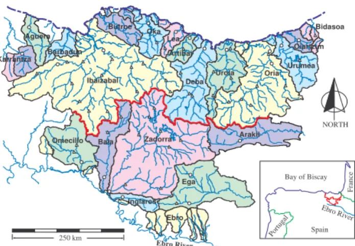
Fig. 1.Division of the study area in 21 systems (different colours) and 41 basins. Thick red line divides the study area into northern and southern basins. Circles and triangles correspond to calibration and validation points, respectively.
complexity. Nevertheless, the ability to generalize these find-ings to ungauged regions remains unsolved. However, in this paper the extrapolation of the parameters to ungauged basins with a hydrological distributed model is successfully exposed.
Knowing water budgets for the basin and its subbasins allows water-resource managers to identify areas of great-est concern in the basin and make more informed decisions about conservation and remediation. A Regional Water Re-sources study was performed at basins within and draining to the Basque Country Region (N of Spain), with a total area of approximately 8500 km2. The objective was to obtain daily and monthly long-term discharges in 567 points (initially 123 points, but at the end of the project more simulation points were demanded), obviously most of them ungauged, with basin areas ranging from 0.25 to 1850 km2. The study area is officially divided into 21 hydrological systems with a to-tal of 41 basins (Fig. 1), only 17 of them with at least one flow gauge station. Northern basins drain to the Bay of Bis-cay in the Atlantic Ocean with a humid climate, and southern basins drain to the Ebro River (which flows to the Mediter-ranean Sea) with a dry continental climate.
In this study, distributed modelling was proposed mainly:
– Due to the high number of simulation points and its vague definition at the beginning of the project. – In order to extrapolate the calibrations at gauged points
to the ungauged ones, without parameters regionaliza-tion but reproducing the natural spatial variability of the Hydrological Cycle.
– Because spatial information is available to be used in this type of models.
Distributed models divide the catchment into a number of smaller areas (grid elements or subcatchments), which are as-sumed to be uniform with respect to their hydrologic parame-ters. There has been an “exponentially growing” recent inter-est in distributed hydrologic modelling that has been fuelled by growing availability of GIS-related information (Schaake, 2003).
Temporal and spatial heterogeneity can be important in many hydrologic applications. The main processes of the hydrological cycle are variable in time and space. The tem-poral variation is observed in input temtem-poral data as precip-itation, potential evapotranspiration, temperature, etc. The spatial variation is mainly detected in soil properties, soil moisture, land use, etc., which are represented as maps. In some cases, simple aggregation of temporal variability can misrepresent important physical processes. Different hydro-logical processes as runoff production and channel network routing are affected by this temporal and spatial variability which must be considered in the selected model (Wood et al., 1988; Gan and Biftu, 1996).
Heuvelmans et al. (2004) studied the spatial variability of soil parameters using regionalisation schemes and concluded that clustering of parameter sets gives a more accurate re-sult than the single parameter approach and is, therefore, the preferred technique for use in the parameterisation of un-gauged sub-catchments as part of the simulation of a large river basin.
The scale effect by spatial and temporal aggregation of nonlinear processes is complex because the mean process re-sponse is not the result of the true mean parameter; therefore it is necessary to introduce effective parameters in the model in order to overcome this problem. The effective parameters usually are: physically senseless, non-stationary (they are not valid if used at different ranges obtained during calibration), and highly uncertain. The proposed solution is to use dis-tributed modelling with a small temporal discretization.
The TETIS model is a freeware which has been devel-oped at DIHMA-UPV as a continuous and event model and corresponds to a distributed hydrological conceptual model, which has been chosen because of their very good perfor-mance in different basins and climates; V´elez (2001), V´elez et al. (2002a, b, 2007) and Franc´es et al. (2007). The TETIS model uses the kinematic wave methodology coupled to the basin geomorphologic characteristics in order to route the flow along the channel network. This procedure is known, according to V´elez (2001), as the “Geomorphologic Kine-matic Wave” or GKW.
conceptual models have a great capacity to compensate for errors and they are difficult to calibrate because they have been created for specific conditions. Sorooshian et al. (1993) indicate that conceptual rainfall-runoff models are difficult to calibrate using automatic methodologies. The successful application of a conceptual rainfall-runoff model depends on how well the model is calibrated.
Beven (1989) has presented the limitations of current rainfall-runoff models and argued that the possible way for-ward must be based on a realistic assessment of predictive uncertainty. For this reason, Beven (1989) has pointed out that many distributed models are just lumped parameter mod-els with a finer mesh, and a closer correspondence between model equations and field processes. This author also indi-cates that long-term records are required, which not always are available. In addition, the calibration must be performed under a physical point of view in order to interpret properly the parameters and to give them a correct interpretation to the spatial variability.
According to Beven (2000), the calibration of a model takes the same characteristics of an adjustment as a multi-ple regression, where the ideal parameters will be such that minimize the residual errors, but if there are residual errors it implies that uncertainty exists in the calibrated model. An important limitation of conceptual models, according to Gan and Burges (1990), is that they are not interpolative and there is no guarantee that the model predicts exactly a value dur-ing validation when it is used beyond the range of calibration. Likewise, it is recommended that a model should be tried in a range drastically different from that they used during the calibration.
The challenge is to estimate the best parameters set of distributed conceptual models. Due to the inability to ac-curately measure distributed physical properties of environ-mental systems, calibration against observed data is typi-cally performed, which is most often achieved with limited rainfall-runoff data. The equifinality noted by Beven (1989) indicates that given the complexity of such models, many different combinations of parameter values may simulate the discharge equally well. These parameter sets may be lo-cated throughout many areas of the parameter space (Duan et al., 1992; Beven, 1989). This uncertainty of the appro-priate parameter values yields predictive uncertainty, as has been demonstrated through applications of the Generalized Likelihood Uncertainty Estimation methodology (Beven and Binley, 1992; Freer et al., 1996; Beven, 2000).
Lid´en and Harlin (2000) mentioned that the risk of obtain-ing a bad model performance, in a conceptual rainfall-runoff model, increases as the initial state moisture condition dimin-ishes.
According to Refsgaard and Knudsen (1996), the main cri-teria for the evaluation of the performance of hydrological models include the joint visualization of the observed and simulated hydrographs, the general water balance, the effi-ciency coefficients and the dispersion graphs.
Efficiency indexes must be treated with care in the mod-els, since reliability and validity are not equivalent and the first one does not imply the second one, increasing the size of a sample does not make the estimation more precise with regard to the simulation, it only diminishes the standard de-viation. It is also true that a model cannot be estimated re-liably based on a small sample, and even if a longer sample is obtained, it does not guarantee a more precise simulation (Duckstein et al., 1985).
The validation process is in charge of demonstrating that physical dominant processes in the basin have been simu-lated appropriately in a specific site. After validation the model is capable of performing predictions that satisfy the precision criteria previously established (Klemeˇs, 1988; Ref-sgaard and Knudsen, 1996; Senarath et al., 2000; Andersen et al., 2001). A fundamental principle in the validation pro-cess is that the model must be validated for the same type of applications for which it was originally developed (Klemeˇs, 1986). In addition, the information used during validation must be different enough from that used during calibration.
The purpose of this paper is to show a Regional Wa-ter Resources application using distributed conceptual mod-elling. The initial parameter maps are estimated using avail-able information and then these maps can be globally cor-rected without losing their internal variability. This split-parameter structure allows for an extrapolating split-parameter from gauged sites to ungauged points using advantages of distributed models.
In the next section a brief description of the TETIS model is performed. Then the split-parameter structure and auto-matic calibration methodology are presented where the ini-tial estimation of spaini-tial parameters is briefly described. The altitude effect on the rainfall is presented and calibration re-sults are exposed jointly with validation and simulation. Fi-nally, some discussion issues and main conclusions obtained during the Water Resources Regional study are exposed.
2 Model description
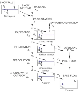
The TETIS model is a conceptual distributed model where each grid cell represents a tank model with six tanks con-nected among them. A conceptual scheme of the vertical movement of the water at each cell can be observed in the Fig. 2. The relationships among different tanks are dif-ferent for every case, but always simple relationships were used. A more detailed description of the model appears in V´elez (2001), V´elez et al. (2002a, b) and Franc´es et al. (2007).
Aquifer Gravitational
storage Surface storage
Static storage Snowpack
Channel
RAINFALL
PRECIPITATION
EVAPOTRANSPIRATION
OVERLAND FLOW SNOWFALL
EXCEDENCE
INFILTRATION
PERCOLATION
GROUNDWATER OUTFLOW
INTERFLOW
BASE FLOW SNOW
MELTING
X
Y
H
1
1
X
Y H
2
2 2
X
Y H
3
3 3
X
Y H
4
4 4
X
H
5
5
X Y
H 0
0 0
T
T2
T3
T4
T5 T0
1 1
Hu
Fig. 2.Runoff production in TETIS model and conceptual scheme of vertical movement at cell scale (Franc´es et al., 2007).
flow exiting is the evapotranspiration. This tank also repre-sents the initial abstractions and pond surfaces. The surface storage is the third tank, where the available water that is not infiltrated can be drained superficially as overland flow. The soil infiltration capacity has been associated with the soil saturated hydraulic conductivity. The fourth tank represents the gravitational storage; the percolation process is modelled according to both soil saturation conditions and the transport capacity, in vertical sense; the remaining water is available to feed the interflow. The fifth tank corresponds to the aquifer, where the vertical flow represents the system groundwater outflow and the horizontal flow is the base flow. Last tank represent the channel at the cell, where each cell is connected to the downstream cell according to the drainage network. Indeed, it is a three-dimensional model. In the Fig. 3 the be-havior of the horizontal flow in TETIS model is observed. All cells drain towards the downstream cell until they reach the channel. Once the channel is reached the flow routing is performed according to the GKW methodology.
The time series required during the model execution are discharge, rainfall, evapotranspiration, snow water equiva-lent and temperature in case that the snow exists. Carto-graphic information uses raster format maps. Digital Terrain Model (DTM) and soil properties (available water and satu-rated hydraulic conductivities) are obtained based on soils studies, land use, geological maps, edaphologic informa-tion, hydrogeological data and other environmental topics that could be interesting and are available at the study area.
Fig. 3. Three-dimensional scheme of TETIS model indicating the horizontal movement among cells (V´elez, 2001).
The infiltration model and the flow channel routing model proposed in TETIS include a few correction factors which correct globally for the different soil properties maps instead of each cell value of the calibration maps, thus reducing dras-tically the number of factors to be calibrated. This strategy allows for a fast and agile modification in different hydro-logical processes. These correction factors can be found us-ing an automatic calibration. In general, if the TETIS model has been calibrated adequately these values must not change along the basin, thereby allowing extrapolation to ungauged subbasins.
TETIS model incorporates a correction factor (rainfall in-terpolation factor) which includes the variation of precipita-tion with the altitude. The rainfall interpolaprecipita-tion factor has been calledβand is given in mm/m. In those cases where it is not possible to calibrate the model due to a lack of water in the balance, then the rainfall interpolation factor can be included as an additional variable to be calibrated.
The routing along the channel network was carried out us-ing the GKW, where nine geomorphologic parameters are re-quired, which can be obtained from potential laws. The co-efficients and the exponents of these potential relationships can be obtained with a geomorphologic regional study for hydrological homogeneous zones. The Basque Country Re-gion uses the geomorphologic parameters recommended in scientific literature (Leopold et al., 1964; V´elez, 2001), since a geomorphologic regional study for hydrological homoge-neous zones was not carried out.
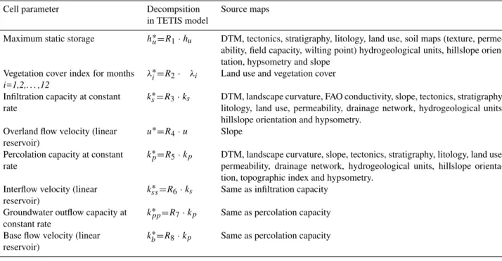
Table 1.Parameter structure and information used for the initial estimation of them at cell scale.
Cell parameter Decompsition Source maps
in TETIS model
Maximum static storage h∗u=R1·hu DTM, tectonics, stratigraphy, litology, land use, soil maps (texture,
perme-ability, field capacity, wilting point) hydrogeological units, hillslope orien-tation, hypsometry and slope
Vegetation cover index for months
i=1,2,. . . ,12
λ∗i=R2· λi Land use and vegetation cover
Infiltration capacity at constant rate
ks∗=R3·ks DTM, landscape curvature, FAO conductivity, slope, tectonics, stratigraphy,
litology, land use, permeability, drainage network, hydrogeological units, hillslope orientation and hypsometry.
Overland flow velocity (linear reservoir)
u∗=R4·u Slope
Percolation capacity at constant rate
kp∗=R5·kp DTM, landscape curvature, slope, tectonics, stratigraphy, litology, land use,
permeability, drainage network, hydrogeological units, hillslope orienta-tion, topographic index and hypsometry.
Interflow velocity (linear reservoir)
kss∗=R6·ks Same as infiltration capacity
Groundwater outflow capacity at constant rate
kpp∗ =R7·kp Same as percolation capacity
Base flow velocity (linear reservoir)
kb∗=R8·kp Same as percolation capacity
a previous period of time to calibrate in order to generate ini-tial soil moisture conditions as real as possible. Normally, a range between one and two months has been used as previous period of time to calibrate to obtain an initial soil moisture condition, also known as a “warm up” period.
The TETIS model uses the inverse distance method to in-terpolate spatially temporal series of rainfall, evapotranspira-tion, temperature and the snow water equivalent. Due to the existence of numerous stations, it is necessary to indicate in the model the number of nearest stations to each cell, to carry out the spatial interpolation.
3 Split-parameter structure and automatic calibration The split-parameter structure refers to the way the model estimate the parameters maps. The parameter estimation methodology tries to distinguish between the effective pa-rameter used in the model at cell scale, and the watershed characteristic estimated from the available information, be-ing the best estimation without losbe-ing its physical meanbe-ing. The relationship between them can be considered as a cor-rection function or, in its simple form, a corcor-rection factor (Franc´es et al., 2007).
Initially, the maps are estimated a priori using environmen-tal and available information (Puricelli, 2003). Then, correc-tion factors are used to modify globally the previously esti-mated maps. In this way, the spatial variability captured in the initial estimated maps is kept and a global change in mag-nitude of parameter maps is performed with correction
fac-tors (Franc´es et al., 2007). This approach reduces drastically the number of parameter to be calibrated, because only the common correction factors are calibrated instead of parame-ter maps (number of parameparame-ters times the number of cells). The correction factor can take into account the model input errors, the temporal and spatial scale effects and the water-shed characteristics. Therefore, it is reasonable to assume that the correction factor is the same for each parameter to all cells within the watershed. Finally, the calibration of the correction factors is performed if there are available observed episodes.
According to the hydraulic behavior at cell scale, the re-quired maps and correction factors are related in Table 1, where it can be found a brief description of the parameter structure and the information used during the initial estima-tion of the parameter maps. The required maps are the max-imum static storage or available water Hu, the vegetation cover index mapλv, the saturated hydraulic conductivity of
soilks, the overland flow velocityvh, and the saturated
hy-draulic conductivity of subsoilkp. The flow velocityv(t )is
calculated according to the GKW procedure and correction factorsR1, R2, . . . ,R9must be calibrated.
The next sections are dedicated to outline briefly the initial estimation of parameter maps and the calibration strategy. 3.1 The initial estimation of spatial parameters
Internal variability Modal value Punctual value 1
2
3 Soil Type I
Soil Type II
A'
A
Limit between cartographic units A' A
ks=0.03 cm/h
(modal value)ks=1.5 cm/h ks variability between cartographic units
Expected spatial variability for ks (modal value)
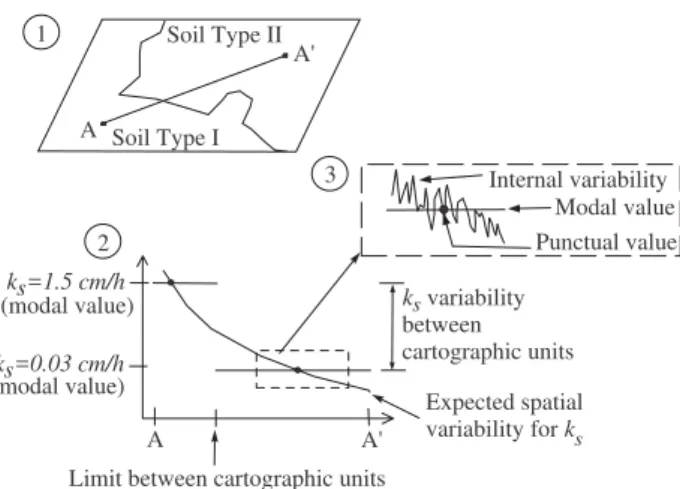
Fig. 4. Spatial variability between cartographic units (Puricelli, 2003).
conductivities of soil and subsoil, respectively. This prior es-timation is made of edaphologic and not strictly edaphologic information, based on available data. This implies the in-terpretation (or inference) of the land properties (Abbaspour and Moon, 1992), extending the analysis to ground mean values. This work requires the knowledge of factors affect-ing the selected variables and their impact. The statistical technique used during the map estimation is the multivari-ate weighted least square method, in which the three hydro-logical parameters were related to environmental variables, deduced from available information.
The proposed procedure was carried out in four stages: 1) Describing land properties showing their spatial variations. 2) Establishing a sampling criterion to obtain a discrete set of representative values at the work area. 3) Defining the general tendency of expected values. 4) Finally, obtaining the thematic maps of physical soil properties.
The cartographic representations of environmental vari-ables, land characteristic and soil properties are related to elements of the landscape. Such elements are related to the spatial distribution of hydrological properties. Consequently, it is possible to define two types of variables:
a) Main variables: directly related to the hydrologic be-havior as soil and subsoil hydraulic conductivity and available water.
b) Environmental variables: those variables capable of ex-plaining part of the spatial variability of main variables. The objective of the initial estimation is to obtain as reli-able as possible the estimation of three main varireli-ables (max-imum available water and saturated hydraulic conductivities of soil and subsoil, respectively). Consequently, a reason-able way to analyze its spatial variability is based on its rela-tion with environmental variables. In real life, the available environmental variables are geology, land use and edaphol-ogy, which use categorical scales and are plotted on a map
by means of cartographic units. Thus, for example, in the case of litology, the categories correspond to the different types of rocks described in the geologic map. Each cate-gory has associated a set of values corresponding to different physical properties, which are based on continuous scales of values. This association is actually stored into a database, where each cartographic unit is a record and properties are the different fields, including modal values. It is considered that the spatial variability of soil properties is significantly smaller within each cartographic unit than among adjacent units.
In Fig. 4 these concepts are exposed graphically. A small region can be observed in the part (1), whose physical prop-erties are expressed at two cartographic units. According to cross section A-A’, the variability of a physical property (ks)
between the cartographic units can be observed in part (2). Thus, it can also be verified that it is possible to define a gen-eral tendency of the values throughout this profile according to the expected spatial variability. Finally, if a cartographic unit is isolated, as shown in part (3), then it can be veri-fied that a variability among the unit exists, which oscillates around its modal value.
The distributed hydrological models force one to use dif-ferent physical properties extracted from the cartographic units. This implies an interpretation and process of the cate-gorical information in order to incorporate its variation.
The most significant environmental variables able to ex-plain the spatial distribution and the variability of the satu-rated hydraulic conductivity are: topographic index, slope, curvature, cumulative area and geology (McKenzie and Austin, 1993; Boer et al., 1996).
The relationship between the vegetation and the landscape has been extracted from DTM (Bolstad et al., 1998). The vegetation is a variable influenced by different edaphic qual-ities including the land use and vegetation coverage.
Once we’ve obtained the thematic layers corresponding to the main and environmental variables, the sampling scheme was based on assigning the modal value of each main vari-able to a portion of land which was considered as a sampling site. This portion of land is obtained from the intersection between all the cartographic units.
The mean values of the main and environmental variables were assigned to the new cartographic units. In the case of the main variables, the assigned weight was the area at each soil cartographic unit, as shown in Fig. 5. In the case of con-tinuous environmental variables, the weight was the average value of all pixels affected by the intersection. The result was a finite number of distributed values on the study area, which represent the values of the main variables based on the spatial distribution of the environmental variables.
Layer A * Layer B *...* Layer N
ks values distributed in
cartographic units
Weight sample distribution at soil cartogrpahic units Soil type I
Soil type II
Fig. 5.Sample weights at cartographic units (Puricelli, 2003).
methodologies such as krigring, incorporating external infor-mation, could be applied to obtain the spatial distribution of the modal values among cartographic units, but those meth-ods were not adopted because they are time-consuming.
The scheme of multivariate weighted least-squares pro-posed by Montgomery and Runger (1996) allows one to com-bine quantitative variables with categorical data and their in-teractions. The objective function to minimize is:
n
X
i=1
ωi yi−β0−
k
X
j=1
βjxij
!
(1)
whereyi is the main variable,xij is the environmental vari-ablej, corresponding to the main variable, ωi is the main
variable weight,β0is the estimation value when all the
en-vironmental variables are null andβi are the environmental
factors.
The dummy variables (also known as indicator variables), are used to incorporate qualitative information in least-squares procedures (Montgomery and Runger, 1996). Thus, a new dummy variable can be defined as the product of the other two dummy variables.
Using this procedure the quantitative information is max-imized, categorical or continuous, being able to incorporate qualitative information and maintaining the coherence with the previous physical knowledge of the main variable.
Finally, the results at each cell are processed using GIS in order to obtain the final thematic layers, adding a spatial term to the original cartographic units according to:
yi∗=yi+E (yi)−yic
(2)
Sinceyi∗is the estimated main variable value at celli,yi is
the main variable value after the multivariate weighted least-squares at each cell in the cartographic unit.E (yi)is the
ex-pected value of the main variable for each cartographic unit,
460000
460000
466000
466000
472000
472000
478000
478000
484000
484000
4702000 4702000
4711000 4711000
4720000 4720000
High : 340 mm
Low : 1 mm
5000
0
NORTH
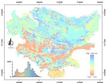
Fig. 6. Results of the initial estimation of parameter map,Hu, in mm. The frequency histogram is in the lower left corner.
andyicis the modal value of the main variable, assigned to each cartographic unit.
In Table 1 are indicated the model parameter (soil proper-ties at cell scale) and the source map used for their estima-tion. Interflow velocity uses the same initial estimation than infiltration capacity, which means than R6 must take into ac-count also the anisotropy between the vertical and horizontal conductivities. Similar for the base flow velocity. With re-spect the groundwater outflow velocity, R7 depends on the basin water balance. A detailed description of each parame-ter estimation and specially the relationship among the main, environmental and dummys variables can be found in Puri-celli (2003).
Finally, three maps of soil parameters are obtained and re-quested by model TETIS. Is shown in Fig. 6 the parameter map (Hu), obtained with the proposed initial estimation
pro-cess, where the spatial variability among the Basque Country Region can be observed.
The GKW parameters can be found in Table 1 of Franc´es et al. (2007).
3.2 Calibration procedure
The calibration of most complex hydrological conceptual models has been performed using traditional manual calibra-tion, using the trial and error as suitable methodology. In this type of calibration it is necessary to be an expert user in order to obtain results in a fast and reliable form. The auto-matic calibration procedures need an initial region of the pa-rameters (physical and feasible values), which can be similar to neighbour basins or hydrologically and climatologically similar basins; Boyle et al. (2000).
the last few years numerous technologies have been devel-oped for the automatic calibration. The methods of global search are the most popular, among them the genetic al-gorithms and the SCE-UA; Madsen (2000). Different au-thors have performed comparisons among different methods, among them the Simulated Annealing, Genetic Algorithm, MultiStart Simplex, MSX and the SCE-UA, emphasizing that the latter behaves better because the obtained parame-ters are more grouped and the number of evaluations of the objective function are lower (Duan et al., 1992; Sorooshian et al., 1993; Duan et al., 1994; Yapo et al., 1998 and Eckhardt and Arnold, 2001). Gan and Biftu (1996) mention that the SCE-UA is ideal to be operated by users who do not know the model and MSX needs an expert user and a process for stages, being more inefficient computationally whereas the SCE-UA obtains results in one execution.
And most recently, the Multiobjective Shuffled Complex Evolution Metropolis algorithm, proposed at the University of Arizona, is best suited for hydrologic model calibration applications that have small parameter sets and small model evaluation times (Tang et al., 2006 and Vrugt et al., 2006).
The model performance criteria in different optimization methods take different execution times, which influences the measurement of their behavior (Thyer et al., 1999). Gan and Burges (1990) mention that the mass balance is the most effi-cient criterion; even tough iterative processes are used. They suggest that there is not an universal and valid scheme to cali-brate a conceptual model following manual or automatic pro-cedures. They recommend as optimization algorithms those based on direct search, considering them to be more robust. Numerous criteria can be found in the literature.
The TETIS model includes different objective function criteria, such as (1) the error in volume (BE), obtained ac-cording to the expression:
BE=Vo− ˆVp
Vo
×100%, (3)
whereVpˆ is the total simulated volume and Vo is the total observed volume. A positive value indicates an underestima-tion and negative values an overestimaunderestima-tion, where zero is the expected value.
(2) The Root Mean Square Error, RMSE. This efficiency criterion is widely used:
RMSE=
v u u u t
n
P
i=1
((Qi− ˆQi)2)
n , (4)
whereQi is the observed discharge at timei,Qiˆ is the simu-lated value at timeiandnis the total number of observations. This criterion looks for the minimum value of RMSE.
(2) The efficiency coefficient,E. It is estimated according to the expression:
E=1−
Pn
i=1(Qˆi−Qi)2
Pn
i=1(Qi− ¯Q)2
, (5)
where, the mean value of the observed discharges is Q¯. This is also known as the efficiency index of Nash and Sut-cliffe (1970). This criterion is commonly used because it involves standardization of the residual variance and its ex-pected value does not change with the length of the record or the runoff magnitude (Kothyari and Singh, 1999). A perfect adjustment suggests a value equal to one; if the value is zero it indicates that the model is not better if it is compared by one variable model (for example, an average value) and neg-ative values indicate that the model behaves worse (Beven, 2000).
Recently, B´ardossy (2007) show how parameter sets can be transferred from gauged basins to close ungauged catch-ments, if performance indexes and annual statistics in donor basins are good. Therefore, after the calibrating process at each basin, the correction factor sets could be used in un-gauged catchments, if parameter map have been estimated previously.
4 Case study: basque country region
The Regional Water Resources study carried out at the Basque Country Region required an intensive information analysis and data process because collected data have dif-ferent resolution, origin, size, quality and quantity. Addi-tionally, other related topics to the case study as rainfall in-crement with altitude, calibration process, validation strategy and simulation are included in this section.
The spatial and temporal quality data analysis was per-formed in order to reduce data uncertainty. This analysis was carried out discarding any doubtful information and cor-recting temporal data if additional information was available. Finally, a field trip along the Basque Country region allowed improving the spatial pattern of soil properties.
4.1 Hydrologic information
The meteorological and hydrological information have been supplied by different entities, namely: the National Me-teorological Institute, INM; the Basque Government, GV; the Navarra Government, GN; the Statutory Deputation of Guipuzcoa, DFG; the Statutory Deputation of Biscay, DFV and the Hydrographic Federation of the Ebro River, CHE.
The discharge information was supplied by twelve differ-ent differ-entities with 143 gauge stations data but just 113 gauge stations were selected, from which 71 stations were used dur-ing the calibration and validation process. It is important to mention some of those stations required to re-establish the natural regime and some flow gauges present a delay with regard to the rain, so it was necessary to realize the respec-tive modification.
The rainfall information consists of a data set of 248 rain gauge stations with a total of 3767 years of daily data. Ad-ditionally, 88 climatological stations were used to estimate the PET. In each cell in the case study the information of the three nearest stations was used in order to estimate the spatial distribution of the input variables.
4.2 The cartographic information
The original spatial information must be digitized in vecto-rial format. The information analysis, estimation methods, spatial distribution of hydrological parameters and final re-sults are processed using GIS tools and databases.
The DTM was supplied with a cell size of 25 m×25 m.
A gross discretization may lead to poor simulation results whereas a very fine discretization would require more input data and significantly increased computation time and space during automatic calibration with little increase in accuracy. Therefore, the cell size selected was 500 m×500 m. This
de-cision implies that the remaining information must be pro-cessed to the same resolution. The DTM was used to extract the basic information: flow direction map to establish con-nectivity among cells, the cumulative drainage area used to estimate flow velocity using GKW procedure, the slope map used to calculate the runoff velocity and flow velocity using GKW method.
In addition, based on available information (Table 1) the needed by TETIS model four parameter maps have been ob-tained: the three main soil characteristics (maximum avail-able water and saturated hydraulic conductivities) and the vegetation index cover map as mentioned in previous sec-tion.
4.3 Rainfall increment with altitude
In those situations in which the precipitation data network does not have rain gauge stations located at high elevations, the main risk is to underestimate the precipitation value at high points. This effect could be possibly the greater source of error in the water balance (Daly et al., 1994).
In the Basque Country Region case study it was initially supposed that the correlation between rainfall and elevation does not exist (β=0.0), which contradicts the observed data on some rain gauge stations. The valley direction can deter-mine the precipitation evolution in some zones of the Basque Country Region. In order to consider the variation of the pre-cipitation with the altitude, it was necessary to estimate this
y = 0.1451x + 1486.2 R2
= 0.0109
800 1000 1200 1400 1600 1800 2000 2200
0 100 200 300 400 500 600 700 800
Elevation (m.a.s.l.)
Annual precipitation (mm)
y = 1.0277x + 983.19 R2
= 0.8019
y = 0.9008x + 1528 R2 = 0.4264
Fig. 7. Relationship between elevation and annual precipitation at Oria River basin. (The circles belong to the lower zone; and tri-angles belong to the upper zone, the continuous line represents the adjustment including all points, the dashed line represents the justment of the lower zone and dashed-dot line represents the ad-justment including the upper zone filled triangle points).
gradient. Part of the supplied data consists of annual rainfall change rates with the elevation above sea level. These rates can be used to estimate a rainfall interpolation factor using the number of rainy days throughout the year. The obtained results were satisfactory once we clarified all the different types of influences on the precipitation.
For example, in the Oria River basin the elevation and precipitation analysis were carried out. If all data are an-alyzed jointly, the influence between precipitation and ele-vation cannot be detected, as shown in the Fig. 7 (continu-ous line). Therefore, the basin has been differentiated in two zones according to the prevailing wind direction. The results of the lower basin zone are shown in Fig. 7 (circle points and dashed line), where the topographic influence is quantifi-able around 90 mm, each 100 m. The constant of the equa-tion indicates a coastal annual precipitaequa-tion of approximately 1500 mm which is coherent with reality. In the upper basin sector (filled triangle and dashed dot line) a remarkable cor-relation is also made visible. It provides similar coefficients to the lower zone; 100 mm, each 100 m.
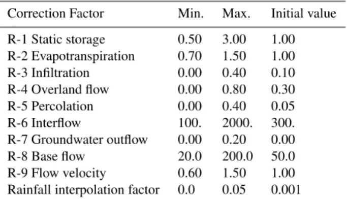
Table 2. Range and initial value of the correction factors used by the SCE-UA calibration method at Basque Country Region.
Correction Factor Min. Max. Initial value
R-1 Static storage 0.50 3.00 1.00
R-2 Evapotranspiration 0.70 1.50 1.00
R-3 Infiltration 0.00 0.40 0.10
R-4 Overland flow 0.00 0.80 0.30
R-5 Percolation 0.00 0.40 0.05
R-6 Interflow 100. 2000. 300.
R-7 Groundwater outflow 0.00 0.20 0.00
R-8 Base flow 20.0 200.0 50.0
R-9 Flow velocity 0.60 1.50 1.00
Rainfall interpolation factor 0.0 0.05 0.001
the necessity to count on rain gauge networks sufficiently ex-tensive to diminish the use of this global factor.
4.4 Automatic calibration
The process of automatic calibration was carried out using the SCE-UA methodology. This procedure was performed independently at every basin or hydrological system, con-sidering that nearby basins must have a hydrological similar behavior. Additionally, during the calibration process as a priori division was proposed, basically because the northern basins must have different behavior than southern basins, but must be similar inside each region.
The TETIS model allows one to choose the objective func-tion during the calibrafunc-tion process, in the case study the RMSE has been selected. In addition, automatic calibration procedures require a search range and the initial values which can be observed in the Table 2. Nevertheless, in every par-ticular case some of these values have been diminished or extended, as the hydrologist considers it suitable. This is quite important because the hydrologist experience and field knowledge are included the calibration process at this point. Concerning to the equifinality problem it was solved using “hydrological sense” in:
1. The search range of each calibration variable (correc-tion factors andβ in the automatic calibration process, Franc´es et al., 2007)
2. A final manual correction of these variables, in most cases with the cost of reducing the calibration efficiency
Therefore, the calibration process requires an iterative pro-cess, where correction factors are estimated automatically using SCE-UA, and then the analysis of the results is per-formed, checking the hydrological sense and the water bal-ance in each hydrological system, in order to reduce the un-certainty associated with the parameter maps and model per-formance. The meaning of ”hydrological sense” refers to the
participation in the calibration process of local experts, the increase of our basins knowledge by several field trips and analyzing carefully the neighbor basins behavior, the basin water balance and the internal flow distribution into the dif-ferent flow components. The initial soil moisture conditions are not included during calibration because a warm-up period of one or two months was included.
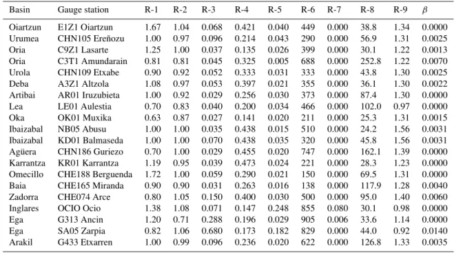
In Table 3 one can see the correction factors and the rain-fall interpolation factor (β)obtained after applying the au-tomatic calibration method SCE-UA. The correction factor variability among basins is not too strong except for correc-tion factors R-3, R-5 andβ. However, important differences can be observed between north and south regions, especially for the mentioned variables. Only two basins were calibrated with groundwater outflow; R-7 is greater than zero and there-foreβ must be zero; both basins located in the south zone. Differences in magnitude among correction factors are ex-plained due to correction factor globally modifies the param-eter map and it is in charge of different hydrological pro-cess. For example, R-3 and R-6 globally correct the parame-ter map (ks), but R-3 is trying to modify the conductivities in order to improve the infiltration process and R-6 is multiply-ing the conductivities in lookmultiply-ing for a good representation of the horizontal flow movement along the cell represented as interflow. In this way the order of magnitude for each cor-rection factor can be explained.
There are two types of correction factor fluctuations among the 20 sets of correction factors shown in Table 3:
1. For correction factor R-7 (groundwater outflow) and forβ; (precipitation increment with altitude) the differ-ences from one basin to another are not random, be-cause these two variables depend on the basin water balance of each basin. In fact, they can not be automat-ically transferred to other basins without a minimum of expert judgment.
2. For the rest of correction factors, the fluctuation is ran-dom (it must be) and reflects the correction factor uncer-tainty produced mainly by the basin differences of each flow gauge station used for calibration:
– Different spatial information (in this case study not different source of information) and inputs (loca-tion, density,. . . ) and their uncertainty.
– Different hydrology at each region, or equivalently, different model conceptualization error.
Table 3.Summary of calibration results at selected gauge stations at Basque Country Region (R: dimensionless correction factors,βis the rainfall interpolation factor in mm/m).
Basin Gauge station R-1 R-2 R-3 R-4 R-5 R-6 R-7 R-8 R-9 β
Oiartzun E1Z1 Oiartzun 1.67 1.04 0.068 0.421 0.040 449 0.000 38.8 1.34 0.0000
Urumea CHN105 Ere˜nozu 1.00 0.97 0.096 0.214 0.043 290 0.000 56.9 1.31 0.0025
Oria C9Z1 Lasarte 1.25 1.00 0.037 0.135 0.026 399 0.000 30.1 1.22 0.0013
Oria C3T1 Amundarain 0.81 0.81 0.045 0.325 0.005 688 0.000 252.8 1.22 0.0070
Urola CHN109 Etxabe 0.90 0.92 0.052 0.333 0.031 333 0.000 43.8 1.30 0.0025
Deba A3Z1 Altzola 1.08 0.97 0.053 0.397 0.021 355 0.000 36.1 1.30 0.0022
Artibai AR01 Iruzubieta 1.00 0.92 0.029 0.256 0.030 373 0.000 87.4 1.30 0.0000
Lea LE01 Aulestia 0.70 0.83 0.040 0.200 0.034 466 0.000 102.0 0.97 0.0000
Oka OK01 Muxika 0.63 0.87 0.027 0.141 0.020 211 0.000 25.3 1.31 0.0015
Ibaizabal NB05 Abusu 1.00 1.00 0.035 0.438 0.015 510 0.000 24.2 1.56 0.0031
Ibaizabal KD01 Balmaseda 1.00 1.00 0.070 0.438 0.035 320 0.000 45.8 1.56 0.0031 Ag¨uera CHN186 Guriezo 0.70 1.00 0.029 0.455 0.020 747 0.000 162.1 1.39 0.0000 Karrantza KR01 Karrantza 1.19 0.95 0.039 0.473 0.024 221 0.000 28.3 1.23 0.0000 Omecillo CHE188 Berguenda 1.72 1.00 0.059 0.290 0.021 150 0.000 69.5 1.31 0.0000
Baia CHE165 Miranda 0.90 0.90 0.031 0.263 0.016 138 0.000 117.9 1.28 0.0040
Zadorra CHE074 Arce 0.80 1.05 0.150 0.400 0.030 500 0.000 95.0 1.40 0.0060
Inglares OCIO Ocio 1.38 1.08 0.071 0.147 0.248 855 0.080 30.1 0.98 0.0000
Ega G313 Ancin 1.20 0.71 0.288 0.196 0.029 905 0.006 33.6 1.14 0.0000
Ega SA05 Zarpia 0.82 1.06 0.680 0.173 0.182 829 0.000 44.0 0.92 0.0140
Arakil G433 Etxarren 1.00 0.99 0.096 0.236 0.020 622 0.000 126.8 1.33 0.0035
Table 4.Summary of water balance after calibration process (PPT: Precipitation, PET: Potential evapotranspiration, RET: Real evapotran-spiration, Q obs: Observed discharge, Q sim: Simulated discharge, UL: Groundwater outflow, DR: Overland flow, IF: Interflow, BF: Base flow, BE: percentage of error in volume, E daily: daily efficiency index and E monthly: monthly efficiency index).
Basin Gauge Area PPT PET RET Q Obs Q Sim UL DR IF BF BE E daily E monthly
station km2 mm/year mm/year mm/year mm/year mm/year mm/year % % % %
Oiartzun E1Z1 Oiartzun 57.25 1975 856 791 1281 1182 0 11 49 40 1.82 0.87 0.96
Urumea CHN105 Ere˜nozu 213.00 2341 829 792 1598 1546 0 3.6 60 37 −5.97 0.82 0.93
Oria C9Z1 Lasarte 805.50 1643 822 754 797 886 0 27 39 35 0.82 0.93 0.98
Oria C3T1 Amundarain 16.25 2167 632 602 1674 1566 0 25 59 16 −13.14 0.68 0.77
Urola CHN109 Etxabe 310.50 1589 794 720 934 867 0 24 41 35 −9.66 0.91 0.96
Deba A3Z1 Altzola 469.00 1597 851 758 636 837 0 28 48 25 −1.99 0.90 0.95
Artibai AR01 Iruzubieta 25.50 1594 800 753 571 838 0 31 41 28 −6.60 0.60 0.67
Lea LE01 Aulestia 37.75 1519 726 664 692 857 0 30 35 35 −4.36 0.78 0.82
Oka OK01 Muxika 28.75 1497 763 671 788 824 0 32 37 31 −3.14 0.81 0.90
Ibaizabal NB05 Abusu 1021.00 1436 924 768 575 667 0 33 43 24 −2.31 0.79 0.90
Ibaizabal KD01 Balmaseda 208.75 1321 897 526 736 793 0 20 43 37 −18.69 0.78 0.78
Ag¨uera CHN186 Guriezo 118.75 1273 799 629 1257 640 0 36 41 23 −36.57 0.73 0.80
Karrantza KR01 Karrantza 114.75 1325 787 687 525 638 0 36 41 23 −6.71 0.86 0.89
Omecillo CHE188 Berguenda 345.75 776 956 529 244 246 0 28 24 47 1.86 0.75 0.94
Baia CHE165 Miranda 306.75 1066 741 547 595 517 0 28 36 36 −12.68 0.81 0.90
Zadorra CHE074 Arce 1358.50 1012 934 518 441 491 0 12 39 49 21.16 0.67 0.90
Inglares OCIO Ocio 86.00 754 1026 596 200 110 48 16 1.4 82 −6.43 0.79 0.77
Ega G313 Ancin 472.50 871 655 487 270 369 14 2.4 28 70 2.59 0.82 0.91
Ega SA05 Zarpia 11.00 1871 967 818 760 1049 0 0 1.5 99 34.07 0.50 0.48
Arakil G433 Etxarren 401.50 1314 765 559 692 751 0 25 45 31 7.87 0.84 0.93
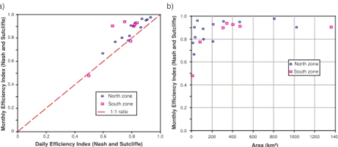
flow is BF, where DR and IF are not as important. These as-pects can be confirmed with land use and cover maps, where forests are located in the north basins and vegetation changes when you move southward. The relief and geomorphologic configuration also contributes to this effect.
0.0 0.2 0.4 0.6 0.8 1.0
0 200 400 600 800 1000 1200 1400
Area (km²)
North zone South zone
0 0.2 0.4 0.6 0.8
0 0.2 0.4 0.6 0.8 1.0
Daily Efficiency Index (Nash and Sutcliffe)
Monthly Efficiency Index (Nash and Sutcliffe)
North zone South zone 1:1 ratio 1.0
a) b)
Monthly Efficiency Index (Nash and Sutcliffe)
Fig. 8. Calibration results, monthly efficiency index versus (a)
Daily efficiency index,(b)Area. (North zone is identified by cir-cles and South zone is represented by small squares).
0 20 40 60 80 100 120 140
Mar-96 Jun-96 Sep-96 Dec-96 Mar-97 Jun-97 Sep-97 Dec-97 Mar-98 Jun-98 Sep-98 Dec-98 Mar-99 Jun-99 Sep-99 Dec-99 Mar-00 Jun-00 Sep-00 Dec-00
Discharges (Hm³)
Observed
Simulated
Fig. 9.Calibration results at “A3Z1 Altzola“ gauge station on Deba River basin, which have been aggregated at monthly scale (Con-tinuous line is the observed flow and dashed line is the simulated flow).
efficiency index. In conclusion, excellent calibrations were obtained in 10 cases (withEdaily over 0.8), acceptable re-sults at 9 basins (Edaily between 0.6 and 0.8) and the one case left was moderate (E daily equal to 0.5); the monthly efficiency indexes show excellent results in most cases.
In Fig. 9 the results are shown after calibration process at “A3Z1 Altzola” gauge station located in Deba River basin, where the error in volume was−1.99%. The performance
efficiency indexes were 0.90 and 0.95 for daily and monthly data, respectively. This calibration results can be considered as excellent.
4.5 Validation process
Distributed models must be validated temporally, spatially and spatial-temporarily, according to the available data. The first case is the validation using the same gauge station used during the calibration but with a different period of time. Spatial validation is performed using the same period of time used during the calibration but in another subbasin, usu-ally located upstream. And the spatial-temporal validation is performed using a different period of time and a differ-ent gauge station. All these validation approaches were per-formed in the Basque Country Region; Table 5 contains the
0.0 0.2 0.4 0.6 0.8 1.0
0 200 400 600 800 1000 1200 1400 North zone South zone 0.0
0.2 0.4 0.6 0.8 1.0
North zone South zone 1:1 ratio
0.0 0.2 0.4 0.6 0.8 1.0
a) b)
Area (km²) Daily Efficiency Index (Nash and Sutcliffe)
Monthly Efficiency Index (Nash and Sutcliffe) Monthly Efficiency Index (Nash and Sutcliffe)
0.0 0.2 0.4 0.6 0.8 1.0
0 100 200 300
c)
Area (km²)
Cofficient of Variation (Monthly Efficiency Index)
1.2
400 y=3.193 x -0.5209
R²=0.997
Fig. 10. Validation results, monthly efficiency index versus (a)
Daily efficiency index and(b)Area. (North zone is identified by circles and South zone is represented by squares points),(c) Coeffi-cient of variation of monthly efficiency index versus area.
summary results, and the validation process was carried out using available data, therefore the validation period length varies from a few months until several years. In those basins with short data length calibration was not carried out and the validation process was performed using the correction fac-tors of the closest more similar basin (i.e. Bidasoa used cor-rection factors from Oiartzun). Northern basins have shown a better performance than southern basins on a daily scale. But the southern basins showed a better efficiency index at the monthly scale. In general, the volume error was greater at the small basins. It was not possible to include all de-tailed validation results in this paper but they can be found at INTECSA-INARSA-UPV (2004).
Table 5 and Fig. 10b show the basin outlet discharge model efficiency (an inverse measure of uncertainty) at gauge sta-tions not used for calibration and for same and different peri-ods to the calibration ones. This model efficiency is represen-tative what will happen simulating the discharges at truly un-gauged points. The model efficiency includes the uncertainty and/or errors in the inputs (precipitation at gauge stations and PET), initial parameters estimation, model conceptualization and parameters calibration. I.e., the objective is to asses the uncertainty of the state variable of interest (which is the in-terest of the end user), not only to estimate the parameter uncertainty.
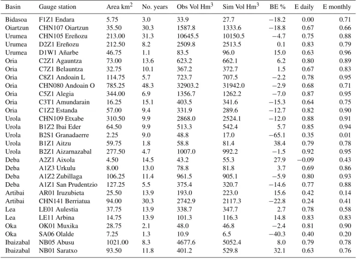
Table 5. Spatial, temporal and spatial-temporal validation results at the Basque Country Region. (No. years: validation period length, Obs Vol: observed volume, Sim Vol: Simulated volume, BE: Error in volume (%), E daily: daily efficiency index and E monthly: monthly efficiency index).
Basin Gauge station Area km2 No. years Obs Vol Hm3 Sim Vol Hm3 BE % E daily E monthly
Bidasoa F1Z1 Endara 5.75 3.0 33.9 27.7 −18.2 0.00 0.71
Oiartzun CHN107 Oiartzun 35.50 30.3 1587.8 1333.6 −18.8 0.67 0.66
Urumea CHN105 Ere˜nozu 213.00 31.3 10645.5 10150.5 −4.7 0.75 0.88
Urumea D2Z1 Ere˜nozu 212.50 8.2 2509.8 2513.5 0.1 0.83 0.79
Urumea D1W1 A˜narbe 46.75 1.1 83.5 96.0 15.0 0.63 0.96
Oria C2Z1 Agauntza 73.00 13.6 623.2 662.1 6.2 0.80 0.89
Oria C7Z1 Belauntza 32.75 10.1 367.2 372.7 1.5 0.67 0.83
Oria C8Z1 Andoain L 114.75 5.7 723.7 707.5 −2.2 0.78 0.95
Oria CHN080 Andoain O 785.25 48.3 32903.2 31942.0 −2.9 0.68 0.71
Oria C5Z1 Alegia 344.00 6.9 1356.7 1262.2 −7.0 0.87 0.95
Oria C3T1 Amundarain 16.25 15.1 403.5 341.6 −15.3 0.64 0.75
Oria C1Z2 Estanda 57.00 9.4 331.9 289.6 −12.7 0.82 0.90
Urola CHN109 Etxabe 310.50 9.9 2868.0 2524.1 −12.0 0.88 0.91
Urola B1Z2 Ibai Eder 64.50 9.9 513.3 542.4 5.7 0.85 0.94
Urola B2S1 Granadaerre 2.25 9.0 48.8 17.0 −65.1 0.35 0.01
Urola B1Z1 Aitzu 59.75 1.8 58.8 81.4 38.4 0.79 0.78
Urola B2Z1 Aizarnazabal 277.50 4.7 1007.0 992.2 −1.5 0.92 0.95
Deba A2Z1 Aixola 4.50 14.5 43.2 55.3 27.9 −0.09 0.43
Deba A1Z3 Urkulu 8.00 13.0 78.8 81.8 3.7 0.69 0.86
Deba A1Z2 Zubillaga 106.25 11.4 961.5 905.1 −5.9 0.80 0.93
Deba A1Z1 San Prudentzio 127.25 5.5 375.4 320.7 −14.6 0.77 0.88
Artibai AR01 Iruzubieta 25.50 13.9 193.0 223.0 15.6 0.42 0.14
Artibai CHN141 Berriatua 94.00 30.3 2742.9 2117.3 −22.8 0.24 0.41
Lea LE01 Aulestia 37.75 13.9 338.7 347.7 2.7 0.78 0.58
Lea LE11 Arbina 14.75 13.9 101.3 116.3 14.8 0.83 0.83
Oka OK01 Muxika 28.75 2.1 48.0 46.8 −2.4 0.81 0.90
Oka SA06 Olalde 7.25 1.3 10.9 6.5 −40.3 0.40 0.20
Ibaizabal NB05 Abusu 1021.00 8.3 4677.6 5052.4 8.0 0.79 0.78
Ibaizabal NB01 Saratxo 93.50 11.8 401.2 529.8 32.1 0.63 0.76
concentrated base flows). The second case is clearly the ini-tial parameter estimation uncertainty: when the basin size is smaller than the scale of the spatial information used for this estimation, it is a “lottery” (the cell parameter estimation un-certainty) to “hit” the actual value (always unknown).
In general, the quality of the southern basins information is poorer than for the northern ones (lower spatial resolu-tions, lower density of input gauges and lower quality of flow gauges). But this is not reflected in the efficiency results, mainly because the other sources of uncertainty have bigger effect on the discharge simulation efficiency.
Figure 10b (and also the Fig. 8b for the calibration) shows a dependence between the variability of the model efficiency and the basin area. It can be shown clearer if we com-pute the coefficient of variation of monthly E for four basin area ranges and plot them versus the intermediate basin area value.
These two dependences can be explained mainly by the initial spatial parameter estimation uncertainty at cell scale. The effect of this uncertainty is maximum for basin area equal to one cell (0.025 km2)and its effect reduces with basin area because the discharge at the outlet is the sum of all cell runoffs within its basin. And by the Central Limit theorem, sums in statistics always reduce the new variability.
If the uncertainty of the simulated discharges at ungauged points is measured by the monthly value of the Nash-Sutcliffe efficiency index (monthlyE) then, the regression equations for the mean monthlyEand its coefficient of vari-ation are very accurate indicators of this model uncertainty for our case study. It must be taken into account that it in-cludes all sources of uncertainty and errors (as explained pre-viously) and can be used as an example for other researches and engineering works.
Table 5.Continued.
Basin Gauge station Area km2 No. years Obs Vol Hm3 Sim Vol Hm3 BE % E daily E monthly
Ibaizabal CHN164 Lemoa 143.75 7.4 905.8 689.1 −23.9 0.54 0.72
Ibaizabal CHN163 Lemona 256.00 30.3 7967.1 6209.0 −22.1 0.49 0.69
Ibaizabal NB04 Zaratamo 522.25 13.4 3268.6 3221.9 −1.4 0.80 0.91
Ibaizabal UNDU Undurraga 31.25 26.9 736.1 723.9 −1.7 0.49 0.64
Ibaizabal IB32 Urkizu 136.50 11.0 815.1 1088.0 33.5 0.73 0.67
Ibaizabal NB11 Orozco 118.00 8.4 484.2 476.8 −1.5 0.71 0.87
Ibaizabal NB02 Gardea 193.50 5.3 363.1 377.6 4.0 0.71 0.92
Ibaizabal IB21 Oromi˜no 20.50 11.0 156.9 172.6 10.0 0.13 −0.31
Ibaizabal CHN175 G¨ue˜nes 258.25 30.3 4789.3 2887.7 −39.7 0.34 0.53
Ibaizabal KD12 Herrer´ıas 258.25 3.7 241.6 288.7 19.5 0.80 0.87
Ibaizabal E. Maro˜no 21.50 13.0 168.0 125.8 −25.1 0.49 0.63
Ibaizabal IB01 Elorrio 29.75 0.3 8.6 8.3 −3.9 0.22 0.27
Ibaizabal IB03 Amorebieta 225.00 2.5 454.8 395.4 −13.1 0.80 0.90
Ibaizabal E. Artziniega 12.00 12.4 89.4 68.4 −23.4 −0.40 −0.18
Karrantza KR01 Karrantza 114.75 13.8 587.7 635.9 8.2 0.29 0.41
Omecillo CHE188 Berguenda 345.75 18.8 1553.9 1428.2 −8.1 0.54 0.72
Omecillo OSM1 Osma−1 79.00 14.8 455.7 482.0 5.7 0.39 0.76
Omecillo OSM2 Osma2 71.50 14.8 273.5 471.5 72.4 0.11 0.36
Baia APRI Aprikano 196.25 11.6 1323.9 1330.0 0.5 0.52 0.72
Baia POBE Pobes 234.50 11.6 1409.7 1500.7 6.5 0.60 0.84
Baia CHE165 Miranda 306.75 20.0 3512.8 3132.1 −10.8 0.49 0.60
Zadorra CHE074 Arce 1358.50 33.1 19722.0 21512.0 9.1 0.65 0.82
Zadorra CHE108 Urrunaga 142.00 44.8 73471.7 57633.3 −21.6 0.40 0.79
Zadorra CHE107 E. Ullibarri 272.50 44.8 7174.7 7016.2 −2.2 0.59 0.87
Zadorra H152 Audicana 89.50 27.0 1168.0 1117.4 −4.3 0.57 0.75
Zadorra H154 Ozaeta 86.00 28.1 1518.8 1688.4 11.2 0.66 0.75
Zadorra CHE221 Larrinoa 19.25 19.0 359.9 283.2 −21.3 0.69 0.73
Zadorra CHE075 Berantevilla 308.00 48.8 5079.9 5312.3 4.6 0.56 0.69
Zadorra H153 Otxandio 34.75 17.3 716.6 468.0 −34.7 0.44 0.67
Zadorra CHE204 Matauko 98.00 8.0 329.5 324.4 −1.6 0.36 0.39
Ega G313 Ancin 472.50 14.3 1777.8 1820.5 2.4 0.78 0.89
Ega G314 Murieta 544.75 14.3 2268.6 2128.9 −6.2 0.73 0.85
Arakil G433 Etxarren 401.50 11.6 3199.4 3110.8 −2.8 0.76 0.88
bad quality information, a scale problem at small basins due to cell size, or strong karstic presence.
Figure 10 shows the behavior of the monthly efficiency in-dex at the basins where the validation has been performed. Those negative indexes that indicate that validation was not satisfactory were not included in the graph. The results in-dicate that the monthly indexes improve with regard to the diaries; same behaviour was reported during calibration. Ac-cording to the monthly efficiency indexes just 11 cases are not satisfactory (Emonthly less than 0.5), 10 are acceptable (E monthly between 0.5 and 0.7) and rest of the 41 cases are excellent (Emonthly over 0.7). On the daily scale 20 cases are not good, 17 can be considered as good and 25 are excellent.
The northern basins show different characteristics among them, at in the case of the Ibaizabal River basin, where the Karrantza and Herradura Rivers show a very different
behav-ior with regard to the nearest Nerbioi and Ibaizabal basins, although the Karrantza River presented poor quality data.
Once the tables were analyzed with the results of the tem-poral, spatial and spatial-temporal validation it is possible to conclude that validation has been performed satisfactorily and it is feasible to proceed with a worthy simulation.
4.6 Long-term simulation
Table 6. Summary of mean results after 40 or 50 years of simulation at ungauged points. PPT: Precipitation in mm/year, PET: Potential evapotranspiration in mm/year, RET: Real evapotranspiration in mm/year, Q sim: Observed discharge in mm/year, V sim: Simulated volume, UL: Groundwater outflow in mm/year, DR: Overland flow, IF: Interflow, BF: Base flow).
Ungauged point Area km2 PPT PET RET Q Sim V Sim Hm3 UL DR % IF % BF %
D. Aldabe 15.50 1843 850 699 1143 17.7 0 26.9 39.0 34.1
D. Endara 19.25 2131 846 801 1327 25.6 0 7.0 52.2 40.9
D. Jaizubia 33.00 1728 857 669 1057 34.9 0 33.6 35.9 30.5
E. San Ant´on 10.75 2187 847 829 1355 14.6 0 8.5 51.6 39.9
D. Oiartzun 81.00 1905 851 750 1153 93.4 0 16.9 45.2 37.9
E. A˜narbe 60.75 2466 826 783 1680 102.1 0 4.6 61.0 34.4
D. Urumea 268.25 2216 816 750 1464 392.7 0 7.7 56.1 36.2
D. Igara 19.25 1516 669 521 994 19.1 0 27.4 38.5 34.1
E. Arrian 9.25 1364 859 790 574 5.3 0 29.7 41.6 28.7
E. Lareo 0.25 1586 748 706 876 0.2 0 27.1 45.2 27.8
E. Ibiur 11.50 1536 846 775 761 8.8 0 23.0 19.5 57.5
D. I˜nurritza 20.00 1467 828 736 732 14.6 0 30.1 42.2 27.7
D. Oria 887.25 1637 820 751 886 786.2 0 27.0 39.0 34.0
E. Ibaieder 29.00 1612 790 741 871 25.2 0 14.0 48.4 37.6
E. Barrendiola 4.00 1662 799 750 909 3.6 0 22.0 46.7 31.3
D. Urola 346.00 1567 792 714 852 294.7 0 24.0 40.7 35.3
E. Aixola 7.75 1734 832 774 958 7.4 0 34.3 40.9 24.8
E. Urkulu 13.00 1582 822 708 873 11.4 0 33.1 18.1 48.8
D. Deba 531.75 1614 851 761 851 452.6 0 29.1 46.8 24.2
D. Saturrar´an 17.25 1597 847 782 815 14.1 0 30.5 40.8 28.6
D. Artibai 106.75 1514 804 747 764 81.6 0 37.3 36.1 26.6
D. Lea 82.00 1422 726 652 771 63.2 0 33.4 28.3 38.3
D. Ea 18.50 1305 723 645 662 12.3 0 22.5 35.4 42.1
D. Oka 184.00 1409 760 665 742 136.6 0 34.9 34.1 31.0
D. Artigas 17.25 1320 761 686 634 10.9 0 22.9 47.4 29.7
D. Laga 12.50 1329 757 672 657 8.2 0 33.1 25.6 41.3
D. Estepona 24.25 1267 885 741 528 12.8 1 17.2 40.1 42.6
correction factors set was validated in the upstream subbasins “A2Z1Aixola”, “A1Z1 San Prudentzio”, “A1Z2 Zubillaga” and “A1Z3 Urkulu”, but the simulation process was also car-ried out in the total basin area at the Bay of Biscay. The same procedure was carried out at all the Country Basque basins and then simulations were performed at 123 points, including calibration and validation points.
The simulation process used the available information from 1951 or 1961 until 2000 and was calculated from all northern basins to the Bay of Biscay, and all southern basins to Ebro River. At each basin the water balance was per-formed. In the case of the Deba River basin (531.75 km2), the mean annual rainfall is 1614 mm, of which the evapo-transpiration is approximately 761 mm, according to TETIS (with PET of 851 mm). The simulated flow value is 851 mm, without losses. The model distributed the flow in 29.1% as overland flow, 46.8% as interflow and 24.6% as base flow. In Fig. 11 one sees the results of the simulation for the 50 stud-ied years. These results indicate that the Deba River basin never exhausts the flow; the recessions are short in time, in-dicating that it is a basin with a permanent flow. A similar
0 40 80 120 160 200
1952 1954 1956 1958 1960 1962 1964 1966 1968 1970 1972 1974 1976 1978 1980 1982 1984 1986 1988 1990 1992 1994 1996 1998 2000
Monthly Discharges (Hm³)
Fig. 11.Simulation results from 1951–2000 at downstream point at Deba River basin.
Table 6.Continued.
Ungauged point Area km2 PPT PET RET Q Sim V Sim Hm3 UL DR % IF % BF %
D. Arcega 5.00 1262 885 716 547 2.7 2 23.1 34.4 42.5
D. Andraka 7.50 1279 886 719 562 4.2 1 43.4 29.6 27.0
D. Butroe 175.00 1324 885 701 625 109.3 1 35.3 31.5 33.2
E. Maro˜no 21.50 1239 935 686 552 11.9 0 34.7 41.9 23.4
D. Ibaizabal 1843.75 1357 908 691 665 1225.6 0 34.8 43.6 21.6
E. Artziniega 12.00 1049 922 436 612 7.3 0 37.0 45.0 18.0
E. Gorostiza 24.75 1588 848 777 809 20.0 0 19.0 60.8 20.2
D. Kadagua 601.75 1236 903 608 627 377.1 0 29.2 50.4 20.4
D. Barbadun 123.75 1235 775 582 654 80.9 1.1 39.5 35.1 25.3
D. Ag¨uera 144.75 1266 801 607 661 95.7 0 39.6 39.5 20.9
D. Ag¨uera CAPV 60.75 1289 790 624 667 40.5 0 40.4 37.4 22.2
D. Calera 38.50 1328.0 790.0 654.0 672 25.9 0 42.3 35.8 21.9
D. Omecillo 354.75 773 956 527 245 86.7 0 28.4 24.7 46.9
E. Gorbea II 10.00 1723 943 772 947 9.5 0 6.5 33.2 60.3
E. Albina 9.75 1324 932 718 602 5.9 0 10.2 49.7 40.1
D. Inglares 97.50 736 1023 581 110 10.7 45 21.3 1.3 77.4
D. Ega CAPV 403.25 832 634 466 352 141.9 13 2.1 28.3 69.6
D. Larrondoa 27.00 1723 970 711 1008 27.2 0 8.4 1.2 90.4
D. Arakil CAPV 85.50 1141 756 530 606 51.8 0 13.1 37.6 49.3
D. Barriobusto 63.75 475 1019 185 289 18.4 0 87.2 4.1 8.7
D. El-Lago 15.25 663 976 457 203 3.1 0 0.7 47.1 52.2
D. Herrera 27.25 554 1005 298 254 6.9 0 64.7 13.3 22.0
D. Riomayor 49.75 525 1004 372 150 7.5 0 11.0 30.6 58.4
D. San Gin´es 75.75 523 1008 350 171 12.9 0 20.1 25.0 54.9
D. Pur´on 27.00 765 900 559 204 5.5 0 32.5 21.4 46.1
D. Valahonda 8.25 575 964 413 160 1.3 0 16.0 48.6 35.4
D. Y´ecora 28.75 466 1031 280 184 5.3 0 60.2 12.0 27.8
5 Discussion and conclusions
In order to solve the equifinality problem it has been pro-posed the use of the “hydrological sense” in: the search range of each calibration variable (correction factors andβ in the automatic calibration process, see Franc´es et al., 2007) and a final manual correction of these variables, in most cases with the cost of reducing the calibration efficiency. The meaning of “hydrological sense” refers to the participation in the cal-ibration process of local experts, the increase of our basins knowledge by several field trips and analyzing carefully the neighbor basins behavior, the basin water balance and the in-ternal flow distribution into the different flow components.
The main advantages in the use of distributed models are the capacity to represent the space variability of hydrological processes and the capacity to understand the main processes at the hillslope and river basin scale. The TETIS model es-timates all hydrological flows that take place at hillslope and river basin scale. In this way, it is possible to explore the origin of the water resources and their implications in wa-ter management. The distributed models are spatially ro-bust because they can give results at any point in the basin, most of them ungauged; they do not aggregate information
and they can be useful at different time scales, from flash flood to water resources management. Another benefit of distributed modelling is the avoidance of the parameter re-gionalization (an implicit process in traditional models). This aspect does not result exclusively in an economic saving but avoids sources of additional errors and uncertainties.
The split-parameter structure proposed is fundamental in order to calibrate the distributed conceptual models, basically because the number of parameters needed calibrate is drasti-cally reduced from cell number times parameter maps to just nine correction factors. But previously it required an initial estimation of parameter maps and then the correction factor calibration could be carried out. Therefore, this parameter structure could be adapted to other distributed models.