www.geosci-model-dev.net/9/2721/2016/ doi:10.5194/gmd-9-2721-2016
© Author(s) 2016. CC Attribution 3.0 License.
RTTOV-gb – adapting the fast radiative transfer model RTTOV for
the assimilation of ground-based microwave radiometer
observations
Francesco De Angelis1, Domenico Cimini2,1, James Hocking3, Pauline Martinet4, and Stefan Kneifel5 1CETEMPS, University of L’Aquila, L’Aquila, Italy
2IMAA-CNR, Potenza, Italy 3Met Office, Exeter, UK
4Météo France – CNRM/GAME, Toulouse, France
5Institute for Geophysics and Meteorology, University of Cologne, Cologne, Germany Correspondence to:Francesco De Angelis ([email protected]) Received: 23 March 2016 – Published in Geosci. Model Dev. Discuss.: 9 May 2016 Revised: 14 July 2016 – Accepted: 27 July 2016 – Published: 19 August 2016
Abstract. Ground-based microwave radiometers (MWRs) offer a new capability to provide continuous observations of the atmospheric thermodynamic state in the planetary bound-ary layer. Thus, they are potential candidates to supplement radiosonde network and satellite data to improve numerical weather prediction (NWP) models through a variational as-similation of their data. However in order to assimilate MWR observations, a fast radiative transfer model is required and such a model is not currently available. This is necessary for going from the model state vector space to the obser-vation space at every obserobser-vation point. The fast radiative transfer model RTTOV is well accepted in the NWP com-munity, though it was developed to simulate satellite ob-servations only. In this work, the RTTOV code has been modified to allow for simulations of ground-based upward-looking microwave sensors. In addition, the tangent linear, adjoint, and K-modules of RTTOV have been adapted to pro-vide Jacobians (i.e., the sensitivity of observations to the at-mospheric thermodynamical state) for ground-based geom-etry. These modules are necessary for the fast minimization of the cost function in a variational assimilation scheme. The proposed ground-based version of RTTOV, called RTTOV-gb, has been validated against accurate and less time-efficient line-by-line radiative transfer models. In the frequency range commonly used for temperature and humidity profiling (22– 60 GHz), root-mean-square brightness temperature differ-ences are smaller than typical MWR uncertainties (∼0.5 K) at all channels used in this analysis. Brightness temperatures
(TBs) computed with RTTOV-gb from radiosonde profiles have been compared with nearly simultaneous and co-located ground-based MWR observations. Differences between sim-ulated and measured TBs are below 0.5 K for all channels ex-cept for the water vapor band, where most of the uncertainty comes from instrumental errors. The Jacobians calculated with the K-module of RTTOV-gb have been compared with those calculated with the brute force technique and those from the line-by-line model ARTS. Jacobians are found to be almost identical, except for liquid water content Jacobians for which a 10 % difference between ARTS and RTTOV-gb at transparent channels around 450 hPa is attributed to dif-ferences in liquid water absorption models. Finally, RTTOV-gb has been applied as the forward model operator within a one-dimensional variational (1D-Var) software tool in an Observing System Simulation Experiment (OSSE). For both temperature and humidity profiles, the 1D-Var with RTTOV-gb improves the retrievals with respect to the NWP model in the first few kilometers from the ground.
1 Introduction
in situ sensors and in the upper troposphere by satellite sounders, there is currently an observational gap in the PBL. According to the WMO Statement Of Guidance For Global Numerical Weather Prediction (WMO, 2014), there are four priorities for atmospheric variables not adequately measured in the PBL: wind profiles, temperature and humidity profiles in cloudy areas, precipitation, and snow mass. Ground-based microwave radiometers (MWRs) provide temperature and humidity profiles in both clear- and cloudy-sky conditions with high temporal resolution and low-to-moderate vertical resolution, with information mostly residing in the PBL (Ci-mini et al., 2006). Ground-based MWRs offer to bridge the current observational gap by providing continuous tempera-ture and humidity profiles in the PBL. When combined with satellite observations, the total information content of the derived atmospheric profiles can be significantly enhanced (Ebell et al., 2013). The data assimilation (DA) of MWR ob-servations into numerical weather prediction (NWP) mod-els may be particularly important in nowcasting and severe weather (fog, convection, turbulence, etc.) initiation. The as-similation of MWR data has been recently investigated (Ci-mini et al., 2014; Caumont et al., 2016), assimilating tem-perature and humidity profile retrievals from a network of 13 MWR members from the international MWRnet network (Cimini et al., 2012). Results showed neutral-to-positive im-pact. However, these experiments used retrieved variables (temperature and humidity profiles), whereas the assimila-tion of raw measurement (TBs) is found to have more impact on the NWP forecasts in the case of satellite data (Geer et al., 2008).
Accordingly, a potential way to increase the impact of MWR DA is to assimilate measured radiance (or bright-ness temperatures, TBs) directly instead of retrieved profiles. With this type of assimilation, all the degrees of freedom for signal of MWRs (Löhnert et al., 2009) can be used to im-prove the NWP model forecast in the PBL. In order to assim-ilate TB, a radiative transfer (RT) forward model is needed. The RT model allows the TB to be computed for selected radiometer channels based on the NWP model state vector. TB differences between the modeled and measured observa-tions can be used within a variational scheme (Courtier et al., 1998) that takes the corresponding uncertainties into account to retrieve temperature and humidity profiles in the first few kilometers from the ground, where MWRs provide the max-imum information content. In addition, the Jacobians (i.e., partial derivatives with respect to the state vector) of the ra-diative transfer model are required to minimize the distances of the atmospheric state from both the first guess and the ob-servations in a variational data assimilation process. These Jacobians represent the sensitivities of observations to the at-mospheric thermodynamical state.
The fast RT model RTTOV (Radiative Transfer for the TIROS Operational Vertical Sounder (TOVS)) is widely used to simulate radiance from space-borne passive sensors. RT-TOV has already been used for many years by many
na-tional meteorological services for assimilating downward-looking observations from visible, infrared, and microwave radiometers, spectrometers, and interferometers (Hocking et al., 2015, and references therein) aboard satellite platforms. The FORTRAN-90 code originally developed at ECMWF in the early 90s (Eyre, 1991) was intended for TOVS direct ra-diance assimilation within three- and four-dimensional varia-tional analysis schemes (3DVAR, 4DVAR). Subsequently the original code has gone through several developments (e.g., Saunders et al., 1999; Matricardi et al., 2001), more recently within the EUMETSAT NWPSAF, of which RTTOV v11.3 is the latest version available. Since its first implementation and throughout its current version, RTTOV has been developed and exploited for satellite observation perspective only. The model allows rapid simulations of radiance for a suite of pas-sive sensors given the atmospheric state vector, i.e., profiles of temperature, gas concentration, cloud liquid water content, and surface properties. The only one variable gas needed for RTTOV v11 in the microwave band is water vapor. An im-portant feature of RTTOV is that, in addition to the forward (or direct) radiative transfer, it also computes the Jacobians, i.e., the gradient of the radiance with respect to the state vec-tor at the location in state space specified by the input state vector values. The Jacobians are calculated in tangent linear (TL), adjoint (AD), and K-modules of RTTOV.
There are other fast RT models used by the NWP commu-nity for satellite data assimilation, like the Commucommu-nity Ra-diative Transfer Model (CRTM – Ding et al., 2011). How-ever, to our knowledge no fast RT model is currently avail-able to simulate ground-based radiometric observations. In this work, version 11.2 of RTTOV has been modified to handle ground-based microwave radiometer observations. The efforts for adapting RTTOV to ground-based observa-tions started within the COST action ES1202 (EG-CLIMET) and have been continued within the COST action ES1303 (TOPROF). The ground-based version of RTTOV developed here, called RTTOV-gb, is able to simulate brightness tem-peratures from ground-based upward-looking microwave ra-diometers. In addition, the TL, AD, and K-modules of RT-TOV have been adapted to provide Jacobians for ground-based geometry. We believe that the availability of RTTOV-gb with its K-module will enable more widespread and better use of MWR observations in NWP models.
2 The formulation of the radiative transfer model 2.1 Radiative transfer model
Given a state vector x (the atmospheric thermodynamical state profile in radiative transfer problem), the radiance vec-tor (or brightness temperature)yis computed as
y=H (x), (1)
whereH is the radiative transfer model (also referred to as the observation operator).
The core of RTTOV-gb simulates ground-based radiome-ter radiance using an approximated form of the radiative transfer equation (RTE) for ground-based (upward-looking) observation geometry:
LATM,i=τi,toa·Bi(TBKG)+ 1
Z
τi,toa
Bi(T )dτ, (2)
whereLATM,iis the radiance at the ground for channeli,
ne-glecting scattering effects,Bi is the Planck radiance at
chan-nel i for a scene temperatureT, τi,toa is the transmittance from the surface to the top of the atmosphere, andTBKGis the microwave cosmic background temperature (2.728 K). Note that in the spectral range under consideration (20–60 GHz), scattering is negligible for particles of the size of atmospheric molecules and cloud droplets, and even for larger ice and snow particles (Kneifel et al., 2010). From a ground-based perspective, the transmittances and optical depths are accu-mulated from the surface to the space instead of from the space to the surface as in the original RTTOV satellite per-spective. Consequently, several subroutines have been modi-fied to reverse the accumulation of transmittances and optical depths through the atmospheric path (see Sect. 6).
The RTE (2) is valid for both clear- and cloudy-sky condi-tions because in the microwave band, RTTOV takes the liq-uid water as an absorbing species into account, and its effects are included through a contribution to the transmittance pro-file. The first term of the right-hand side of the RTE (2) is the cosmic background radiation; the second term is the atmo-spheric contribution.
The RTE (2) has been numerically solved overN spheric levels which are numbered from the top of the atmo-sphere as follows:
– levelj =1, pressurePj=0.005 hPa, temperatureTj= T1, transmittanceτij=τi,toafor channeli;
– levels fromj =2 toj=N−1,Pj are pressures of the
fixed-pressure levels,τijis the surface-to-level
transmit-tance for channeli;
– level j=M, the first level which lies strictly above the input 2 m pressure (i.e.,M <=N andPM < P2 m), τij=τi,Mfor channeli;
– level j=N, PN=1050 hPa, surface air temperature TN=TS,τiN=1 for all channels.
For the ground-based perspective and each channel (omitting theiindex for convenience), we define
1τj =τj+1−τj 1Bj=Bj−Bj+1 1dj =dj−dj+1
, (3)
where1dj is the optical depth of the single layerj, anddj
is the level-to-surface optical depth.
The contribution of the cosmic background radiation is LCOSMIC=τ1·B (TBKG)withτ1=τtoa. (4) The atmospheric contribution is
LA= τM
Z
τLEV=1
B (T )dτ+ST=X1
j=M( τj+1
Z
τj
Bdτ )+ST, (5)
where
τj+1
Z
τj
Bdτ =τj+1Bj+1−τjBj+
1 1dj
1Bj1τj
=1τj· [Bj+1+1Bj
1 1dj] −
τj1Bj, (6)
and ST is the contribution of the first layer above the surface: ST=BS(1−τM)−(BM−BS)+(BM−BS)
·(1−τM)·
1 dM
, (7)
withBS the Planck function evaluated at the input 2 m
tem-perature.
In Eq. (4) we have used a parameterization of the Planck function (i.e., the so-called linear-in-tau assumption, where tau means the optical depth of the single layer, corresponding to1d in the notation used in this study). In the linear-in-tau assumption, the source function throughout the layer is linear with the optical depth of the layer (Saunders, 2010): B[T (1d)]=Bj+1+(Bj−Bj+1)
1d 1dj
, (8)
whereBjis the Planck function for the top of the layer,Bj+1 is the Planck function at the bottom of the layer, and1dj is
the optical depth of the layer. In the ground-based perspec-tive,1d goes from 0 to1dj from the bottom to the top of
the layer.
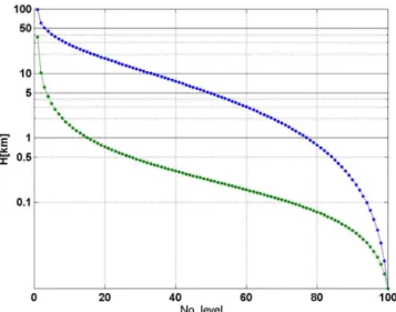
Figure 1.Vertical spacing of profiles levels used for RTTOV in this analysis. Level altitudes and altitude differences between levels are reported respectively with blue and green lines. Note that theyaxis is in logarithmic scale.
2.2 The input atmospheric profiles and near-surface variables
The input profile data may be supplied on an arbitrary set of pressure levels. These consist of vertical profiles of tem-perature (K) and humidity (ppmv) for clear-sky conditions, and additional cloud liquid water content (CLW in kg kg−1) profiles for simulating cloudy conditions. In addition, pres-sure, temperature, and humidity values at 2 m altitude are re-quired. The transmittance calculations described below are performed using atmospheric layers bounded by a number of fixed pressure levels. RTTOV-gb interpolates the input pro-files to the fixed pressure levels for the transmittance calcula-tion, but note that the RTE is integrated in the pressure levels supplied by the user (Hocking, 2014).
Currently RTTOV-gb uses fixed 101 pressure levels from 0.005 to 1050 hPa for the transmittance calculation. These levels have been specifically selected for the ground-based perspective to be denser close to ground (34 levels below 2 km) than those usually used for the satellite perspective. Moreover they were chosen to improve the accuracy of the optical depth prediction scheme used by RTTOV-gb com-pared to that obtained with the levels used for satellite sim-ulations. The vertical spacing of levels is shown in Fig. 1 in terms of level altitude differences.
2.3 Transmittance model
The main variable computed in the radiative transfer model is the atmospheric optical depth for each channeliand for each atmospheric layerj. The optical depths depend on the view-ing angle of the instrument, pressure, temperature, and con-centrations of the absorbing species. The optical depth
differ-ences between adjacent pressure levels are obtained through a linear combination inXkj, the so-called predictors (j
be-ing the level andkthe number of predictors, from 1 toNP).
The predictors are derived from the input state vector profile and depend on the elevation angleθand pressureP, temper-atureT, and specific humidity q at the considered level and the level above that. The optical depth from the surface to the levelj in channelialong a path at an angleθ from the vertical,dij, is obtained as follows:
dij=di,j+1+
P X
k=1
aij kXkj(P , T , q, θ ), (9)
withaij k the regression coefficients between optical depths
and predictors.
The contribution of the water vapor to the optical depth is treated separately from that of uniformly mixed gases al-though they are calculated with two algorithms of the same form. There are three types of predictors for satellite per-spective, predictors 7 (Matricardi et al., 2001), 8 (Matricardi, 2005), and 9 (Saunders, 2010), each of which is better suited for a specific application. The predictors used in RTTOV to parameterize the optical depths refer to the reference temper-ature and specific humidity profiles (i.e., the average of the training profile set, respectivelyTjrefandqjref). Additionally, the number of predictors depends on the selected gas.
We found the predictors 7 to give the best results for the ground-based geometry, and thus they are used herewith to train RTTOV-gb. The predictors 7 and the profile vari-ables involved in the predictors calculation are listed in Ap-pendix A. Note that predictors 7 were originally developed for satellite simulations up to 60◦zenith angles and as such, the errors in the optical depth prediction increase for zenith angles above∼75◦(i.e., for elevation angles below∼15◦). For MWR observations of the PBL thermodynamics, these scanning angles turn out to be crucial because of the infor-mation carried by opaque channels on the PBL temperature profile. Thus, it is foreseen that an alternative set of predic-tors, specific for low-elevation angles in the ground-based geometry, may be worth investigating and developing in the future, though it is beyond the scope of this study.
The coefficientsaikj are calculated by linear regression of
di,j−di,j+1 againstXkj. For the regression, dij are
NW-PSAF profile dataset interpolated on 101 pressure levels, al-ready used for training RTTOV. It is important to empha-size that this profile set was carefully chosen from a set of more than 100 million profiles to represent a wide range of physically realistic atmospheric states (Matricardi, 2008). Transmittances are computed for six selected scanning an-gles which are discussed in Sect. 3.1. We limit the lowest elevation angle used in the training phase to 10◦because of the limitation of the predictors 7 that has already been men-tioned.
If the optical depths for uniformly mixed gases and water vapor aredijM anddijW respectively, the total optical depth is dij=dijM+d
W
ij. (10)
Then, optical depths are converted to transmittances: τij=exp(−dij). (11)
Finally, RTTOV-gb computes the output radiance and TB from the derived transmittances and the input vertical tem-perature profile using the radiative transfer Eq. (2).
2.4 Jacobians: tangent linear, adjoint, and gradient matrix models
The Jacobian matrixKgives the change in radianceδyfor a change in any element of the state vectorδx, assuming a linear relationship about a given atmospheric statex0:
δy=K(x0)δx. (12)
The elements of Kcontain the partial derivatives δyi/δxj,
where the subscriptirefers to the channel andj to the layer number. The Jacobian provides the radiance sensitivity for each channel given unit perturbations at each level of the state vector and in each of the surface parameters. It shows clearly, for a given profile, which layers in the atmosphere are most sensitive to changes in temperature and variable gas concentrations for each channel. The K-module of RTTOV computes theK(x0)matrix for each input profile. Alterna-tively, the Jacobians can be computed with the so-called brute force (BF) method, whereKis estimated by perturbing each element of the atmospheric state vector, repeating the RT-TOV direct module iteratively. However, the calculations of the Jacobians with the BF method are slower and less rigor-ous than with the K-module of RTTOV.
It is not always necessary to store and access the full ma-trix K; thus, the RTTOV package has routines to compute the tangent linear only, i.e., the change in radiance yi for a
given change in atmospheric profileδxaround an initial at-mospheric statex0.
δy(x0)=
δx∂y1
∂x ,δx ∂y2
∂x ,δx ∂y3
∂x . . .δx ∂ynchan
∂x
with ∂
∂x =∇x= ∂ ∂x1 , ∂ ∂x2 , . . ., ∂ ∂xN (13)
Similarly, the adjoint routines compute the change in any quantity of the state vector (e.g.,T,q, surface variables etc.) δxaround an assumed atmospheric statex0, given a change in the radianceδy.
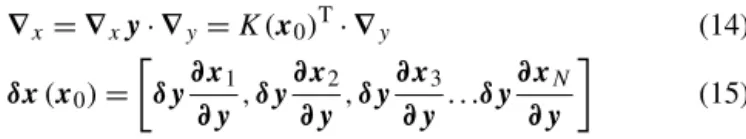
∇x=∇xy·∇y=K(x0)T·∇y (14)
δx(x0)=
δy∂x1
∂y ,δy ∂x2
∂y ,δy ∂x3
∂y . . .δy ∂xN
∂y
(15)
For very large systems, it may be not feasible to calculate the full Jacobian matrixK, and the tangent linear and adjoint operations are computed instead.
The TL code is derived directly from the forward model because it represents the analytic derivative of the radiance (forward model outputs) with respect to the atmospheric state vectorx. The AD code is derived from the TL code. Finally, the K code is obtained from the AD code distributing the AD level derivatives through the number of channels. Before running TL, AD, and K models, the direct model needs to be run because many of the intermediate variables calculated by the direct model are needed by the TL, AD, and K-modules.
3 Performance of RTTOV-gb
The performance of RTTOV-gb has been tested in four dif-ferent ways, reported in the following subsections: validation against the LBL RT model used as reference for the training and against another independent reference LBL RT model (3.1); a comparison of TB simulated with RTTOV-gb from a radiosonde profile dataset with nearly co-located MWR mea-surements (3.2); a comparison of Jacobians calculated with the RTTOV-gb K-module and the brute force method, and also with Jacobians computed with an analytical model (3.3); the exploitation of RTTOV-gb as a forward model operator within a one-dimensional variational scheme (3.4).
3.1 Comparison with line-by-line model computed radiance
To compare RTTOV-gb against the LBL model adopted for the regression training, we computed clear-sky TB with both RTTOV-gb and R98 at selected channels from the set of 83 atmospheric profiles used in the training phase. Result-ing TB differences are a measure of the regression error. Here we focus on the systematic (bias) and root-mean-square (rms) TB differences. We consider 14 channels commonly used by commercial MWRs, in particular the Humidity And Temperature PROfiler (HATPRO, Rose et al., 2005): 22.24, 23.04, 23.84, 25.44, 26.24, 27.84, 31.40, 51.26, 52.28, 53.86, 54.94, 56.66, 57.30, and 58.00 GHz. Channels from 22 to 31 GHz are in the so-called K-band, while channels from 51 to 58 GHz are in the so-called V-band.
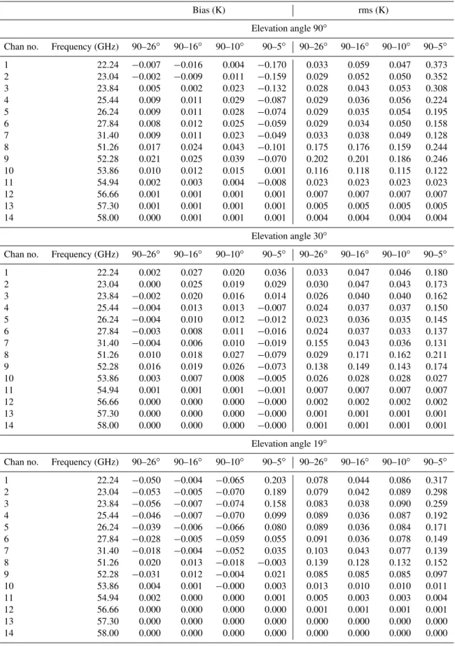
Table 1.Statistics for the comparison between RTTOV-gb and the line-by-line model R98 (Rosenkranz, 1998) at elevation angles 90, 30, 19, and 10◦(R98 minus RTTOV-gb). The HATPRO channel number (Chan no.), the channel central frequency, bias, and rms for each RTTOV training configuration are reported. The values which are larger than 0.5 K are highlighted in bold.
Bias (K) rms (K)
Elevation angle 90◦
Chan no. Frequency (GHz) 90–26◦ 90–16◦ 90–10◦ 90–5◦ 90–26◦ 90–16◦ 90–10◦ 90–5◦
1 22.24 −0.007 −0.016 0.004 −0.170 0.033 0.059 0.047 0.373
2 23.04 −0.002 −0.009 0.011 −0.159 0.029 0.052 0.050 0.352
3 23.84 0.005 0.002 0.023 −0.132 0.028 0.043 0.053 0.308
4 25.44 0.009 0.011 0.029 −0.087 0.029 0.036 0.056 0.224
5 26.24 0.009 0.011 0.028 −0.074 0.029 0.035 0.054 0.195
6 27.84 0.008 0.012 0.025 −0.059 0.029 0.034 0.050 0.158
7 31.40 0.009 0.011 0.023 −0.049 0.033 0.038 0.049 0.128
8 51.26 0.017 0.024 0.043 −0.101 0.175 0.176 0.159 0.244
9 52.28 0.021 0.025 0.039 −0.070 0.202 0.201 0.186 0.246
10 53.86 0.010 0.012 0.015 0.001 0.116 0.118 0.115 0.122
11 54.94 0.002 0.003 0.004 −0.008 0.023 0.023 0.023 0.023
12 56.66 0.001 0.001 0.001 0.001 0.007 0.007 0.007 0.007
13 57.30 0.001 0.001 0.001 0.001 0.005 0.005 0.005 0.005
14 58.00 0.000 0.001 0.001 0.001 0.004 0.004 0.004 0.004
Elevation angle 30◦
Chan no. Frequency (GHz) 90–26◦ 90–16◦ 90–10◦ 90–5◦ 90–26◦ 90–16◦ 90–10◦ 90–5◦
1 22.24 0.002 0.027 0.020 0.036 0.033 0.047 0.046 0.180
2 23.04 0.000 0.025 0.019 0.029 0.030 0.047 0.043 0.173
3 23.84 −0.002 0.020 0.016 0.014 0.026 0.040 0.040 0.162
4 25.44 −0.004 0.013 0.013 −0.007 0.024 0.037 0.037 0.150
5 26.24 −0.004 0.010 0.012 −0.012 0.023 0.036 0.035 0.145
6 27.84 −0.003 0.008 0.011 −0.016 0.024 0.037 0.033 0.137
7 31.40 −0.004 0.006 0.010 −0.019 0.155 0.043 0.036 0.131
8 51.26 0.010 0.018 0.027 −0.079 0.029 0.171 0.162 0.211
9 52.28 0.016 0.019 0.026 −0.073 0.138 0.149 0.143 0.174
10 53.86 0.003 0.007 0.008 −0.005 0.026 0.028 0.028 0.027
11 54.94 0.001 0.001 0.001 −0.001 0.007 0.007 0.007 0.007
12 56.66 0.000 0.000 0.000 −0.000 0.002 0.002 0.002 0.002
13 57.30 0.000 0.000 0.000 −0.000 0.001 0.001 0.001 0.001
14 58.00 0.000 0.000 0.000 −0.000 0.001 0.001 0.001 0.001
Elevation angle 19◦
Chan no. Frequency (GHz) 90–26◦ 90–16◦ 90–10◦ 90–5◦ 90–26◦ 90–16◦ 90–10◦ 90–5◦
1 22.24 −0.050 −0.004 −0.065 0.203 0.078 0.044 0.086 0.317
2 23.04 −0.053 −0.005 −0.070 0.189 0.079 0.042 0.089 0.298
3 23.84 −0.056 −0.007 −0.074 0.158 0.083 0.038 0.090 0.259
4 25.44 −0.046 −0.007 −0.070 0.099 0.089 0.036 0.087 0.192
5 26.24 −0.039 −0.006 −0.066 0.080 0.089 0.036 0.084 0.171
6 27.84 −0.028 −0.005 −0.059 0.055 0.091 0.036 0.078 0.149
7 31.40 −0.018 −0.004 −0.052 0.035 0.103 0.043 0.077 0.139
8 51.26 0.020 0.013 −0.018 −0.003 0.139 0.128 0.132 0.152
9 52.28 −0.031 0.012 −0.004 0.021 0.085 0.085 0.085 0.097
10 53.86 0.004 0.001 −0.000 0.003 0.013 0.010 0.010 0.011
11 54.94 0.002 0.000 0.000 0.001 0.005 0.003 0.003 0.004
12 56.66 0.000 0.000 0.000 0.000 0.001 0.001 0.001 0.001
13 57.30 0.000 0.000 0.000 0.000 0.000 0.000 0.000 0.000
Table 1.Continued.
Bias (K) rms (K)
Elevation angle 10◦
Chan no. Frequency (GHz) 90–26◦ 90–16◦ 90–10◦ 90–5◦ 90–26◦ 90–16◦ 90–10◦ 90–5◦
1 22.24 −0.299 −0.324 −0.626 −0.930 0.428 0.381 0.681 1.035
2 23.04 −0.297 −0.317 −0.632 −0.955 0.461 0.369 0.685 1.027
3 23.84 −0.391 −0.312 −0.648 −0.998 0.662 0.356 0.698 1.067
4 25.44 −0.544 −0.294 −0.664 −1.055 1.214 0.343 0.716 1.128
5 26.24 −0.573 −0.284 −0.663 −1.065 1.414 0.342 0.718 1.143
6 27.84 −0.592 −0.270 −0.659 −1.075 1.685 0.349 0.716 1.159
7 31.40 −0.594 −0.260 −0.680 −1.129 2.023 0.377 0.731 1.205
8 51.26 0.000 −0.088 −0.337 −0.609 0.272 0.103 0.350 0.633
9 52.28 −0.021 −0.029 −0.106 −0.202 0.083 0.034 0.112 0.214
10 53.86 0.022 0.000 −0.007 −0.014 0.037 0.003 0.011 0.021
11 54.94 0.005 0.000 −0.002 −0.004 0.009 0.001 0.003 0.006
12 56.66 0.000 0.000 −0.000 −0.000 0.001 0.000 0.000 0.001
13 57.30 0.000 0.000 −0.000 −0.000 0.000 0.000 0.000 0.001
14 58.00 0.000 0.000 −0.000 −0.000 0.000 0.000 0.000 0.000
Figure 2. (a1)TB at K-band channels (20–35 GHz) computed by RTTOV-gb (red stars) and LBL R98 (black stars) from profile no. 8 of the dependent set.(a2)Same as(a1), but for V-band channels (50–60 GHz).(b1)TB differences (R98 minus RTTOV-gb) at K-band channels. (b2)Same as(b1), but for V-band channels.
for regression training (predictors 7 are used). This compari-son allow us to investigate the best performing combination. The four sets of elevation angles are 90–53–42–35–30–26◦; 90–42–30–24–19–16◦; 90–42–30–24–19–10◦; and 90–42– 30–19–10–5◦.
Bias and rms are lower than the manufacturer error speci-fication for HATPRO channels (∼0.5 K – Rose et al., 2005) for all the considered training sets and elevation angles, with the exception of 22–31 GHz channels at 10◦elevation angle with the training sets 90–26, 90–10, and 90–5◦. This result seems to confirm that predictors 7 are not ideal for elevation angles lower than 15◦. However, it is encouraging to note that even at 10◦, bias and rms are within the instrumental error for all the channels when the training set 90–16◦is adopted. Note that the agreement at low-elevation angles is better for the V-band opaque channels, which are most important for
PBL temperature retrieval. Table 1 shows that the best among the considered training configurations is the set of elevation angles from 90 to 16◦. Somewhat surprising, this configura-tion gives acceptable results even at 10◦, despite this eleva-tion angle being outside the training angle range.
Figure 2 shows two spectra computed at HATPRO chan-nels by RTTOV-gb and LBL R98 for the same atmospheric profile belonging to the dependent set. For this particular case, TB differences between the two models are within 0.1 K for all channels.
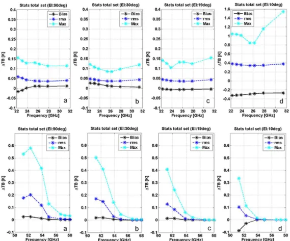
Figure 3.Bias (black solid line), rms (blue dashed line), and maximum (cyan dashed line) of TB difference between RTTOV-gb and LBL R98 (Rosenkranz, 1998) for the dependent 83-profile set and the best training configuration (R98 minus RTTOV-gb). Top panels: K-band channels; bottom panels: V-band channels. Panels(a),(b),(c), and(d)report results at 90, 30, 19, and 10◦elevation angle, respectively. Note that the top panel(d)has a differentyaxis scale with respect to the other top panels.
K-band (22–31 GHz), while they are 0.003 and 0.025 K for the V-band opaque channels (54–58 GHz). For these chan-nels the maximum difference does not exceed 0.15 K. The agreement is slightly worse at transparent V-band channels (51–54 GHz), with bias, rms, and maximum difference re-spectively within 0.03, 0.2, and 0.6 K. The larger discrepan-cies at transparent V-band channels are probably due to the combined influence of temperature and water vapor, which likely decreases the correlation of layer opacity with the two thermodynamical variables. Similar results are found for other elevation angles, such as 30 and 19◦. Note that the er-ror statistics at 90◦ elevation (i.e., zenith) are about 1 order of magnitude larger than the analogous statistics of the orig-inal nadir-looking RTTOV (Saunders, 2002, 2010). We be-lieve the reason is the behavior of the two terms contributing to the total radiance (Eq. 2), i.e., the background and the at-mospheric contributions. Uncertainty in atat-mospheric optical depth, as those induced by regression, will influence the to-tal radiance through the effects on these two terms. For the satellite (downward-looking) case, these effects tend to com-pensate due to a warmer background (e.g., overestimated op-tical depths cause more emission from the atmosphere but
less contribution from the relative warmer background). Con-versely, for the ground-based perspective there is no com-pensation of the two terms because of the cold cosmic back-ground (e.g., overestimated optical depths causes more emis-sion from the atmosphere and less contribution from the rel-ative colder background).
Figure 3 shows bias, rms, and maximum difference respec-tively up to−0.3, 0.4, and 1.5 K for K-band channels at 10◦ elevation. These are significantly larger compared to higher elevation angles. This is attributed to the use of predictors 7, which are not designed for elevation angles lower than 15◦. This may also be due to the fact that 10◦is outside the eleva-tion angle range used in the training configuraeleva-tion (90–16◦). However, Table 1 shows that extending the range of training elevation angles to 10◦or less generally degrades statistics. In any case, we highlight that the rms errors in Fig. 3 are smaller than the uncertainty associated with TB observations (∼0.5 K) for all channels and all elevation angles.
Table 2.Statistics for the comparison between RTTOV-gb and the line-by-line model R98 (Rosenkranz, 1998) with the best RTTOV training configuration and the independent profile set (R98 minus RTTOV-gb). HATPRO channel number (Chan no.), the channel central frequency, bias, and rms at elevation angles 90, 30, 19, and 10◦are reported.
Training configuration: elevation angles from 90 to 16◦
Bias (K) rms (K)
Chan no. Frequency (GHz) 90◦ 30◦ 19◦ 10◦ 90◦ 30◦ 19◦ 10◦
1 22.24 −0.008 0.021 −0.004 −0.282 0.049 0.045 0.042 0.326
2 23.04 −0.002 0.020 −0.006 −0.276 0.042 0.045 0.042 0.319
3 23.84 0.007 0.017 −0.008 −0.273 0.035 0.044 0.045 0.320
4 25.44 0.018 0.001 −0.009 −0.257 0.032 0.042 0.051 0.339
5 26.24 0.011 0.007 −0.009 −0.247 0.031 0.041 0.052 0.342
6 27.84 0.009 0.004 −0.008 −0.232 0.031 0.040 0.053 0.346
7 31.40 0.008 0.001 −0.010 −0.230 0.036 0.046 0.061 0.365
8 51.26 −0.004 −0.017 −0.015 −0.094 0.156 0.159 0.127 0.115 9 52.28 −0.004 −0.009 −0.004 −0.033 0.169 0.131 0.076 0.039 10 53.86 −0.001 0.002 −0.001 −0.002 0.095 0.025 0.015 0.012
11 54.94 0.002 0.000 −0.000 −0.000 0.023 0.011 0.008 0.003
12 56.66 0.002 0.000 0.000 0.000 0.010 0.004 0.002 0.000
13 57.30 0.001 0.000 0.000 0.000 0.009 0.003 0.001 0.000
14 58.00 0.001 0.000 0.000 0.000 0.008 0.002 0.001 0.000
R98 minus RTTOV-gb TB differences are shown in Fig. 4. Results are for the best training configuration and for eleva-tion angles 90, 30, 19, and 10◦. Statistics are similar to those obtained with the dependent profile set. In this case, how-ever, the error statistics are of the same order of magnitude as the analogous performance of the original nadir-looking RT-TOV with an independent profile set (Saunders, 2002, 2010). For elevation angles down to 19◦, biases range from less than 0.002 K for the opaque channels to 0.020 K for K-band, while rms is less than 0.060 K for K-band and 0.025 K for the opaque channels. The maximum TB differences do not exceed 0.5 K. Similarly to the test with the dependent profile set, larger discrepancies are found in the transparent V-band channels (51–54 GHz) and for K-band channels at 10◦ eleva-tion. All the statistics obtained with the independent profile set and the best training configuration are summarized in Ta-ble 2. Consistently with the dependent test, the independent test in Fig. 4 and Table 2 confirms that the rms errors are smaller than the uncertainty associated with TB observations for all channels and all elevation angles.
The previous tests against the reference LBL R98 model have also been performed at the 22 frequency channels (22– 60 GHz) used by another commercial microwave radiome-ter, the MP-3000A (Cimini et al., 2011, 2015). Statistics, re-ported in Table 3 in terms of bias and rms, are similar to those obtained for HATPRO channels, at both K- and V-band.
Note that LBL R98 is the model used to train the re-gression scheme. In order to perform a completely inde-pendent test, we compare RTTOV-gb with an indeinde-pendent reference radiative transfer model, the Atmospheric Radia-tive Transfer Simulator (ARTS, Buehler et al., 2005;
Eriks-son et al., 2011; EriksEriks-son and Buehler, 2015), and a com-pletely different profile dataset. In this test, HATPRO ob-servations are simulated using RTTOV-gb and ARTS from a set of 1327 thermodynamic profiles from the AROME anal-ysis over Bordeaux from April to October 2014. AROME is the French convective-scale NWP model with a 2.5 km horizontal grid mesh developed by Météo France (Seity et al., 2010). Both clear- and cloudy-sky conditions are consid-ered. This dataset, which is limited in space, time, and thus in atmospheric conditions, was chosen to demonstrate the per-formance of RTTOV-gb in typical deployment environment. Since the goal of this analysis is to test the fast RT model-ing (RTTOV-gb) with respect to accurate LBL calculation, all other settings being equal, ARTS settings for absorption model have been selected to adopt the same absorption model as RTTOV-gb as much as possible: R98 for oxygen and wa-ter vapor absorption, and the model described in Liebe et al. (1993) for cloud liquid water (referred as MPM93 within ARTS). Note that MPM93 is the only option for liquid water absorption available in ARTS. Conversely RTTOV-gb is con-sistent with the original RTTOV, which adopts a combination of Liebe et al. (1991) and Lamkaouchy et al. (1997) models (English et al., 1999).
Figure 4.Same as Fig. 3 but for the independent 52-profile set (R98 minus RTTOV-gb). Top panels: K-band channels; bottom panels: V-band channels. Panels(a),(b),(c), and(d)report results at 90, 30, 19, and 10◦elevation angle, respectively. Note that top panel(d)has a different
yaxis scale to the other top panels.
for V-band opaque channels (55–58 GHz). Similar to previ-ous tests, larger discrepancies are found in the more trans-parent V-band channels (51–54 GHz) with an rms error up to 0.5 K at 51 GHz in cloudy-sky; but here the rms is dom-inated by a bias contribution induced by systematic differ-ences found between LBL and ARTS at these three chan-nels (∼0.3–0.5 K, not shown). This may be caused by small differences in the implementation of the R98 gas absorp-tion and/or the radiative transfer code. This issue is currently under investigation, though its understanding goes beyond the scope of this paper. Comparing Figs. 4 and 5, we no-tice slightly larger differences (by 0.1–0.2 K) in the RTTOV-gb vs. ARTS than in the RTTOV-RTTOV-gb vs. R98 tests. We at-tribute this to the fact that RTTOV-gb is totally independent of ARTS and moreover to the specific profile dataset, which likely introduces biases with respect to the RTTOV-gb train-ing climatology. Note that TB differences for all the channels are of the same order of magnitude as those found between ARTS and the original nadir-looking RTTOV (Buehler et al., 2006). This demonstrates comparable capabilities between RTTOV-gb and the original version of RTTOV. The rms TB differences between RTTOV-gb and ARTS at 90◦elevation are within 0.5 K, thus below the uncertainty associated with
TB observations. From the three tests above, we can con-clude that in the elevation angle range from 90 to 10◦, the forward model error due to the use of the fast RT with re-spect to the reference LBL model is within the instrument uncertainty. This confirms that RTTOV-gb can be safely de-ployed in place of an LBL model into variational assimilation schemes.
3.2 Comparison with real observations
(HAT-Table 3.Statistics for the comparison between RTTOV-gb and the line-by-line model R98 at MP-3000A channels with the best RTTOV training configuration, for both the dependent (top) and independent (bottom) profile set (R98 minus RTTOV-gb). MP3000A channel number (Chan no.), the channel central frequency, bias, and rms at elevation angles 90, 30, 19, and 10◦are reported.
Dependent profile set
Bias (K) rms (K)
Chan no. Frequency (GHz) 90◦ 30◦ 19◦ 10◦ 90◦ 30◦ 19◦ 10◦
1 22.23 −0.016 0.027 −0.004 −0.319 0.059 0.047 0.044 0.376
2 22.50 −0.015 0.026 −0.004 −0.321 0.058 0.047 0.044 0.378
3 23.03 −0.009 0.025 −0.005 −0.318 0.053 0.045 0.042 0.370
4 23.83 0.002 0.020 −0.007 −0.313 0.043 0.040 0.038 0.357
5 25.00 0.010 0.014 −0.007 −0.300 0.039 0.037 0.037 0.346
6 26.23 0.011 0.010 −0.006 −0.284 0.037 0.036 0.036 0.343
7 28.00 0.011 0.008 −0.005 −0.270 0.036 0.037 0.037 0.3500
8 30.00 0.011 0.006 −0.004 −0.266 0.038 0.040 0.040 0.366
9 51.25 0.024 0.018 0.013 −0.088 0.177 0.171 0.128 0.104
10 51.76 0.024 0.019 0.013 −0.056 0.189 0.164 0.111 0.066
11 52.28 0.025 0.019 0.012 −0.029 0.203 0.149 0.085 0.034
12 52.80 0.029 0.020 0.008 −0.011 0.207 0.116 0.052 0.014
13 53.37 0.019 0.017 0.002 −0.002 0.181 0.068 0.022 0.005
14 53.85 0.012 0.007 0.001 0.000 0.120 0.029 0.010 0.003
15 54.40 0.006 −0.000 0.001 0.000 0.055 0.012 0.006 0.002
16 54.94 0.004 0.001 0.000 0.000 0.023 0.007 0.003 0.001
17 55.50 0.002 0.001 0.000 −0.000 0.013 0.004 0.002 0.000
18 56.02 0.001 0.000 0.000 −0.000 0.009 0.003 0.001 0.000
19 56.66 0.001 0.000 0.000 −0.000 0.007 0.002 0.000 0.000
20 57.29 0.001 0.000 −0.000 −0.000 0.005 0.001 0.000 0.000
21 57.96 0.001 0.000 −0.000 −0.000 0.004 0.001 0.000 0.000
22 58.80 0.000 0.000 −0.000 −0.000 0.004 0.001 0.000 0.000
Independent profile set
Bias (K) rms (K)
Chan no. Frequency (GHz) 90◦ 30◦ 19◦ 10◦ 90◦ 30◦ 19◦ 10◦
1 22.23 −0.008 0.022 −0.003 −0.284 0.049 0.046 0.042 0.157
2 22.50 −0.008 0.021 −0.005 −0.279 0.048 0.046 0.043 0.158
3 23.03 −0.002 0.020 −0.006 −0.277 0.042 0.045 0.042 0.154
4 23.83 0.007 0.017 −0.008 −0.274 0.035 0.044 0.045 0.164
5 25.00 0.012 0.011 −0.009 −0.263 0.033 0.043 0.051 0.206
6 26.23 0.011 0.007 −0.009 −0.247 0.031 0.041 0.052 0.236
7 28.00 0.010 0.004 −0.008 −0.232 0.031 0.040 0.053 0.257
8 30.00 0.008 0.002 −0.009 −0.228 0.033 0.043 0.057 0.273
9 51.25 −0.005 −0.018 −0.016 −0.094 0.156 0.160 0.128 0.067 10 51.76 −0.005 −0.014 −0.010 −0.061 0.162 0.149 0.105 0.039 11 52.28 −0.005 −0.009 −0.004 −0.037 0.170 0.131 0.077 0.020 12 52.80 −0.004 0.000 −0.001 −0.015 0.169 0.098 0.044 0.015 13 53.37 −0.003 0.007 −0.003 −0.005 0.145 0.056 0.021 0.015 14 53.85 −0.002 0.002 −0.002 −0.002 0.097 0.026 0.015 0.012 15 54.40 0.000 −0.002 −0.001 −0.001 0.047 0.015 0.011 0.007
16 54.94 0.002 0.000 −0.000 −0.000 0.023 0.011 0.008 0.003
17 55.50 0.002 0.000 0.000 −0.000 0.016 0.007 0.005 0.001
18 56.02 0.002 0.000 0.000 −0.000 0.013 0.005 0.003 0.001
19 56.66 0.001 0.000 0.000 0.000 0.010 0.004 0.002 0.000
20 57.29 0.000 0.000 0.000 0.000 0.009 0.003 0.001 0.000
21 57.96 0.000 0.000 0.000 0.000 0.008 0.002 0.000 0.000
Figure 5.Bias (black solid line), standard deviation (red dashed line), and rms (blue dashed line) of TB differences between RTTOV-gb and the reference radiative transfer model ARTS (Eriksson and Buehler, 2015), for both clear(a1–2)and cloudy(b1–2)sky conditions (ARTS minus RTTOV-gb). Panels(a1, b1–a2, b2)are for K- and V-band channels, respectively. All panels report results at 90◦elevation angle.
PRO) operated at the radiosonde launching site. The dataset was first reduced to clear-sky conditions. To be conserva-tive, clear-sky conditions have been selected using three-fold screening, based on (i) ceilomenter cloud base height (CBH), (ii) sky infrared temperature (TIR), and (iii) 20 min stan-dard deviation of liquid water path (σLWP)from HATPRO. Thus, periods with CBH below maximum range (8000 m), TIR>−30◦C, orσLWP>10−2kg m−3were rejected. More-over, cases with integrated water vapor differences between microwave radiometer and radiosonde profiles larger than 1 mm have been discarded in order to reduce instrumental un-certainties involved in the comparison. After this screening, only 23 profiles remained for the analysis. Bias, standard de-viation, and rms differences between TB observed by the mi-crowave radiometer and simulated with both RTTOV-gb and ARTS are shown in Fig. 6. With respect to the MWR obser-vations, RTTOV-gb shows bias from 0.02 K at 22.24 GHz to 0.5 K at 23.84 GHz in the K-band and from 0.16 to 0.31 K in the V-band opaque channels. The rms errors range from 0.90 to 0.47 K in the K-band and from 0.41 to 0.64 K in the V-band opaque channels. Larger bias is found at V-band transparent channels: 1–2 K at 51.26 GHz and 4–5 K at 52.28 GHz with either gb or ARTS simulations. Note that RTTOV-gb and ARTS show similar statistics with respect to MWR observations. This result is very important as it suggests that forward model errors due to the fast model approximation are not dominant. Note that bias values of the same order of magnitude for the 51–54 GHz range were previously re-ported (Hewison et al., 2006; Löhnert and Maier, 2012; Mar-tinet et al., 2015; Blumberg et al., 2015), employing MWRs of different types and manufacturers. This may be attributed to a combination of uncertainties from instrument calibration and gas absorption models. In fact, semi-transparent chan-nels (as in the 51–54 GHz range) suffer from larger cali-bration uncertainties due to the lack of a close reference-temperature calibration point. In addition, their response is influenced by the water vapor continuum and oxygen line
Figure 6.Bias (black line), standard deviation (red line), and rms (blue line) of differences between TB measured with the microwave radiometer and TB simulated from radiosonde profiles respectively with RTTOV-gb (solid lines) and the reference radiative transfer model ARTS (dashed lines), both for clear-sky conditions at 90◦ elevation angle (measurements minus simulations).
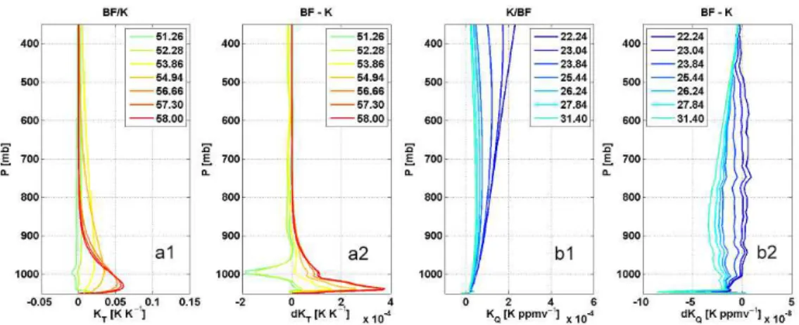
Figure 7.Jacobians calculated with the RTTOV-gb BF method and K-module.(a1)Temperature Jacobians for V-band channels;(b1)absolute humidity for K-band channels. Note that the BF method (solid line) and K-module (dashed line) are not distinguishable as they nearly completely overlap. Panels(a2, b2)show Jacobian differences between BF and K, for temperature and absolute humidity respectively.
3.3 Comparison of Jacobians
After testing the RTTOV-gb direct module, the RTTOV-gb Jacobians calculation needs to be tested in order to provide a complete tool for a fast and safe MWR data assimilation. First, a consistency test of the Jacobians calculated with TL-, AD-, and K-modules of RTTOV-gb has been performed to ensure the correctness of the TL/AD/K coding modified for a ground-based perspective. The test resulted in nearly the same Jacobians for TL, AD-, and K-modules. Subsequently, the temperature and humidity Jacobians calculated with the RTTOV-gb K-module have been compared with those com-puted with the brute force (BF) method for a specific cloudy-sky profile. The BF method calculates the Jacobian by finite differences by calling the direct module multiple times after perturbing each individual input profile variable. The consis-tency of K-module with BF was confirmed using the RTTOV test suite (Brunel and Hocking, 2014), bearing in mind that some small differences between the Jacobians are expected. Figure 7 shows the temperature and absolute humidity Jaco-bians for the V- and K-bands channels. The JacoJaco-bians com-puted with RTTOV-gb BF and K-module are almost identical with differences smaller than 1 %. As expected, the TB sen-sitivity to atmospheric temperature is higher in the low tropo-sphere, especially in the PBL, and it increases with frequency in the spectral range between 51 and 58 GHz. Between 22 and 31 GHz, the sensitivity of the TBs to water vapor is al-most independent of altitude and decreases with increasing frequency.
The Jacobians for cloud liquid water (CLW) are needed when cloudy-sky conditions are considered. Figure 8 shows a comparison of CLW Jacobians calculated with the RTTOV-gb K-module and the BF method. Similar to temperature and humidity, they are found to be almost identical (differences smaller than 0.1 %, likely due to truncation errors). As ex-pected, the TB sensitivity to CLW increases with frequency in the K-band, while it decreases with frequency in the
V-Figure 8.Cloud liquid water Jacobians calculated with the RTTOV-gb BF method and K-module (left) and Jacobian differences be-tween BF and K (right), for K-band (top) and V-band (bottom) chan-nels, respectively. Note that the BF method (solid) and K-module (dashed) are not distinguishable as they nearly completely overlap.
band due to the increasingly dominant oxygen absorption. TBs are sensitive to CLW at all levels up to 322 hPa (about 10 km), where RTTOV, and thus also RTTOV-gb, have set their upper limit for non-zero CLW.
RTTOV-Figure 9.As in Fig. 7, but for Jacobians calculated with ARTS (solid line) and the RTTOV-gb K-module (dashed line). Panels(a2, b2)show Jacobian differences between ARTS and RTTOV-gb K-module, for temperature and absolute humidity respectively.
Figure 10.As in Fig. 8, but for Jacobians calculated with ARTS (solid line) and the RTTOV-gb K-module (dashed line).
gb. These are similar to each other, both in shape and order of magnitude, from the surface up to 322 hPa (RTTOV cloud limit). However, differences of about 10 % occur around 450 hPa, particularly at transparent channels (31, 51, and 52 GHz). These are likely due to small differences in the liq-uid water absorption models in ARTS and in RTTOV-gb, as mentioned above in Sect. 3.1. However, for a typical CLW profile, these model differences lead to small TB differences (order of 0.1 K) and are thus deemed as negligible.
3.4 1D-Var application
Finally, RTTOV-gb has been tested as a forward model within a one-dimensional variational (1D-Var) scheme. For this purpose, the 1D-Var software package provided by the NWPSAF (Weston, 2014) has been adapted in the framework of the COST Action TOPROF to exploit RTTOV-gb. Among other modifications, the 1D-Var tool has been modified to
al-low the assimilation of observations at different elevation an-gles for the same instrument. The 1D-Var approach searches the atmospheric statex that minimizes both the distance to the backgroundxband the observationy. The cost function J needs to be minimized, modifying the different variables defined in the control vectorx(Cimini et al., 2010):
J=1 2
y−H (x)T R−1
y−H (x)
+1
2[x−xb] TB−1[x
−xb]. (16)
Here B represents the background-error covariance matrix andRthe observation error covariance matrix.H represents the observation operator, in our case RTTOV-gb. The back-ground profile comes from a short-range forecast of an NWP model or from a co-located radiosonde. Here,xbis a 3 h fore-cast from the French convective-scale model AROME. The Jacobians needed to minimize the cost functionJ are calcu-lated with the RTTOV-gb K-module.
ob-servation errors to the RTTOV-gb simulations. The synthetic random errors are assumed to follow a diagonal R matrix with reasonable standard deviations, i.e., ∼0.2–1.0 K de-pending on channels (Hewison, 2007).
In clear-sky conditions, temperature and specific humidity are used as control variables in the 1D-Var. A comparison between temperature and humidity retrievals obtained with 1D-Var and the corresponding unperturbed and background profiles for two retrieval examples are shown in Fig. 11. As expected, the 1D-Var retrievals are closer to the truth than the background profiles. In this case 1-D-Var provides an im-provement with respect to the background in the first 2 km for temperature and in the first 4 km for humidity, which is en-couraging for future data assimilation experiments. A com-prehensive evaluation of RTTOV-gb plus 1D-Var for data as-similation using real MWR observations will be the subject of future work.
Here, we just underline that the main advantage of RTTOV-gb with respect to LBL models is the considerably lower computation time. Of course the priority of LBL mod-els is more accuracy than speed, though settings may be tuned to improve the computation performances. Although a detailed analysis on computation speed goes beyond the scope of this paper, we found that RTTOV-gb is faster than our implementation of ARTS (Martinet et al., 2015) for both the direct and Jacobian calculations. Moreover, our tests demonstrate that the computation time for Jacobians is shorter by a factor of 8 for the RTTOV-gb K-module than for the direct module with the brute force method.
4 Summary
Version 11.2 of the fast radiative transfer model RTTOV, de-veloped for space-borne sensors, has been successfully mod-ified to simulate ground-based microwave radiometer ob-servations. In addition to the direct module, which allows ground-based MWR observations to be simulated, the TL-, AD-, and K-modules of RTTOV have been modified in or-der to provide temperature, humidity, and cloud liquid wa-ter Jacobians for the ground-based perspective. We intro-duced the ground-based version of RTTOV, called RTTOV-gb, and demonstrated its potential for fast MWR TB simula-tions from thermodynamic profiles. RTTOV-gb has been val-idated against accurate, but less time-efficient, reference line-by-line models and real MWR observations. Results demon-strate its applicability as a forward model within a variational scheme for fast and safe MWR data assimilation into NWP models. It is believed that the direct assimilation of TB, in-stead of retrieved profiles, may improve the impact of MWR observations for temperature and humidity profiles analysis in the first few kilometers from the ground, where MWRs provide the maximum information content.
The performance of RTTOV-gb has been validated by comparison with TB simulated with the line-by-line model
R98 (Rosenkranz, 1998), the same model as used for the RTTOV training phase. For both dependent and independent profile sets, rms errors are below the typical TB uncertainty of ground-based MWRs (∼0.5 K), ranging from a maximum of 0.06 K for the water vapor band to 0.025 K for the V-band opaque channels. Larger discrepancies are observed at the transparent V-band channels (51 and 52 GHz), with an rms within 0.20 K, and at elevation angle 10◦. TBs simulated with RTTOV-gb from AROME analyses have also been compared with those simulated with the reference line-by-line model ARTS. At 90◦elevation, for both clear- and cloudy-sky con-ditions TB differences do not exceed 0.25 K in terms of bi-ases and rms at all HATPRO channels except for the trans-parent V-band channels 51–52 GHz (up to 0.5 K in cloudy-sky conditions). Finally, RTTOV-gb has been validated by radiosonde-derived TB with real nearly collocated MWR ob-servations. In this case, the rms error increases with respect to the RTTOV-gb/LBL comparisons, ranging from 0.90 to 0.47 K in the K-band and from 0.41 to 0.64 K in the V-band opaque channels. Larger discrepancies were found at V-band transparent channels, which may be explained by calibration and gas absorption uncertainties. However, the statistics of RTTOV-gb and ARTS simulations with respect to MWR ob-servations are similar for each channel, suggesting that for-ward model errors due to the fast model approximation are not dominant. Temperature, humidity, and cloud liquid water Jacobians computed with RTTOV-gb K-modules were found to be similar in shape and magnitude with those calculated with the brute force method or with the ARTS model.
Finally, RTTOV-gb has been tested as a forward model within a 1D-Var software package in an OSSE to improve AROME thermodynamic profiles estimated by directly as-similating synthetic MWR TB. For both temperature and humidity profiles, the 1D-Var considerably improves the re-trievals with respect to the background, in the first few kilo-meters from the ground. Concerning the computation speed, RTTOV-gb with K-module is found to be 8 times faster in computing Jacobians than the brute force method. As ex-pected, RTTOV-gb is demonstrated to be faster than the line-by-line models such as ARTS for both the direct and the Ja-cobians calculation.
Figure 11.Temperature(a)and humidity(b)profiles of background (blue line), truth (red line), and 1D-Var retrievals (cyan line) for two clear-sky profiles.
5 Code and data availability
The original RTTOV v11.2 can be obtained via the re-quest form on the NWPSAF website (NWPSAF, 2013; http: //nwpsaf.eu/site/software/rttov/rttov-v11/).
The efforts for adapting RTTOV to ground-based obser-vations started within the COST (http://www.cost.eu/) action ES1202 (EG-CLIMET) and have been con-tinued within the COST action ES1303 (TOPROF, http://www.toprof.eu/). The modifications needed to adapt the radiative transfer equation from the satellite-to the ground-based perspective have been made in the subroutine src/main/rttov_integrate.F90. The RTTOV sub-routines that have been modified in RTTOV-gb to reverse the way that transmittances and optical depths are initial-ized and accumulated are src/main/rttov_transmit.F90 and src/main/rttov_opdep.F90 respectively. The calculation of the predictors 7 for the ground-based perspective has been adapted in the subroutine src/main/rttov_profaux.F90. Modifications made in the direct module of RT-TOV v11.2 code have been imported in the cor-responding TL-, AD-, and K-modules’ subroutines
(i.e., rttov_integrate_tl.F90, rttov_integrate_ad.F90, rttov_integrate_k.F90; rttov_transmit_tl.F90, rt-tov_transmit_ad.F90, rttov_transmit_k.F90; rt-tov_opdep_l.F90, rttov_opdep_ad.F90, rttov_opdep_k.F90). The conditions of release of RTTOV-gb are currently under discussion among NWPSAF and COST action TOPROF. This may happen through an integration of RTTOV-gb into future RTTOV releases or as a stand-alone package disseminated through the TOPROF website.
All the information needed to download the ARTS code can be found on the website: http://www.radiativetransfer. org/.
The NWPSAF profiles, from which we interpolated the profile sets used for the RTTOV-gb training and indepen-dent test, are available at https://nwpsaf.eu/deliverables/rtm/ profile_datasets.html.
Appendix A
The predictors Xkj introduced in Sect. 2 are functions of
the absorbing gas, the zenith angle θ, the pressure, temper-ature, and water vapor mixing ratio profiles, and finally the reference temperature and water vapor mixing ratio profiles (i.e., the average of the training profile set). These are de-fined in Matricardi et al. (2001) and briefly summarized be-low. Introducing at each fixed levelj the pressurePprof(j ), the temperature, and the water vapor mixing ratio Tprof(j ) andWprof(j ), and the corresponding referenceTref(j )and Wref(j ), the following variables are defined:
T (j )=hTprof(j )+Tprof(j+1)i/2 T∗(j )=hTref(j )+Tref(j+1)i/2 W (j )=hWprof(j )+Wprof(j+1)i/2 W∗(j )=hWref(j )+Wref(j+1)i/2 P (j )=hPprof(j )+Pprof(j+1)i/2 Tr(j )=T (j )/T∗(j )
δT (j )=T (j )−T∗(j )
Wr(j )=W (j )/W∗(j )
Tw(j )= j X
l=N−1
P (l+1)[P (l+1)−P (l)]Tr(l+1),
withTw(j=N )=0 at the surface. Ww(j )=
( j X
l=N−1
P (l+1)[P (l+1)−P (l)]W (l) )
.
( j X
l=N−1
P (l+1)[P (l+1)−P (l)]W∗(l) )
The RTTOV predictors 7 are derived from the variables above as listed in Table A1.
Table A1.Predictors 7 used for mixed gases and water vapor (after Matricardi et al., 2001).
Predictor 7 Mixed gases Water vapor
X1,j sin(θ ) sin2(θ )Wr2(j )
X2,j sin2(θ ) (sin(θ )Ww(j ))2
X3,j sin(θ )Tr(j ) (sin(θ )Ww(j ))4
X4,j sin(θ )Tr2(j ) sin(θ )Wr(j )δT (j )
X5,j Tr(j ) √sin(θ )Wr(j )
X6,j Tr2(j ) 4
√
sin(θ )Wr(j )
X7,j sin(θ )Tw(j ) sin(θ )Wr(j )
X8,j sin(θ )TTwr(j )(j ) (sin(θ )Wr(j ))
3
X9,j √sin(θ ) (sin(θ )Wr(j ))4
X10,j √sin(θ )√4Tw(j ) sin(θ ) Wr(j ) δT (j )|δT (j )|
X11,j 0 √sin(θ )Wr(j )δT (j )
X12,j 0 (sin(θ )Wr(j ))
2
Ww
X13,j 0
√
sin(θ )Wr(j )Wr(j )
Ww(j )
X14,j 0 sin(θ )W
2
r(j )
Tr(j )
X15,j 0 sin(θ )W
2
r(j )
T4
Acknowledgements. This work has been stimulated through the COST Action ES1303 (TOPROF), supported by COST (European Cooperation in Science and Technology). Part of the work was supported by the EU H2020 project GAIA-CLIM (Ares(2014)3708963/Project 640276). The authors would like to acknowledge the NWPSAF and Met Office, in particular Peter Rayer, for providing support with RTTOV coding, and Météo France, for providing AROME analyses and measurements performed in the Bordeaux campaigns.
Edited by: K. Gierens
Reviewed by: two anonymous referees
References
Blumberg, W. G., Turner, D. D., Löhnert, U., and Castleberry, S.: Ground-Based Temperature and Humidity Profiling Using Spectral Infrared and Microwave Observations. Part II: Actual Retrieval Performance in Clear-Sky and Cloudy Conditions, J. Appl. Meteorol. Clim., 54, 2305–2319, doi:10.1175/JAMC-D-15-0005.1, 2015.
Boukabara S. A., Clough, S. A., Moncet, J.-L., Krupnov, A. F., Tretyakov, M. Yu., and Parshin, V. V.: Uncertainties in the Tem-perature Dependence of the Line-Coupling Parameters of the Mi-crowave Oxygen Band: Impact Study, IEEE T. Geosci. Remote Sens., 43, 1109–1114, doi:10.1109/TGRS.2004.839654, 2005. Brousseau, P., Berre, L., Bouttier, F., and Desroziers, G.:
Back-ground error covariances for a convective scale data assimilation system: AROME 3D-Var, Q. J. Roy. Meteor. Soc., 137, 409–422, 2011.
Brunel, P. and Hocking, J.: RTTOV v11 Test Suite, Met Office Doc ID: NWPSAF-MO-TV-031, 2014.
Buehler, S. A., Eriksson, P., Kuhn, T., von Engeln, A., and Verdes, C.: ARTS, the Atmospheric Radiative Trans-fer Simulator, J. Quant. Spectrosc. Ra., 91, 65–93, doi:10.1016/j.jqsrt.2004.05.051, 2005.
Buehler, S. A., Courcoux, N., and John, V. O.: Radiative transfer calculations for a passive microwave satellite sensor: Comparing a fast model and a line-by-line model, J. Geophys. Res., 111, D20304, doi:10.1029/2005JD006552, 2006.
Cadeddu, M. P., Payne, V. H., Clough, S. A., Cady-Pereira, K., and Liljegren, J. C.: The effect of the oxygen line-parameter modeling on temperature and humidity retrievals from ground-based microwave radiometers, IEEE T. Geosci. Remote Sens., 45, 2216–2223, 2007.
Caumont, O., Cimini, D., Löhnert, U., Alados-Arboledas, L., Bleisch, R., Buffa, F., Ferrario, M. E., Haefele, A., Huet, T., Madonna, F., and Pace, G.: Assimilation of humidity and tem-perature observations retrieved from ground-based microwave radiometers into a convective-scale NWP model, Q. J. Roy. Me-teor. Soc., doi:10.1002/qj.2860, 2016.
Cimini, D., Hewison, T. J., Martin, L., Güldner, J., Gaffard, C., and Marzano, F.: Temperature and humidity profile retrievals from groundbased microwave radiometers during TUC, Meteorol. Z., 15, 45–56, 2006.
Cimini, D., Westwater, E. R., and Gasiewski, A. J.: Tempera-ture and Humidity Profiling in the Arctic Using Ground-Based
Millimeter-Wave Radiometry and 1DVAR, IEEE T. Geosci. Re-mote Sens., 48, 1381–1388, 2010.
Cimini, D., Campos, E., Ware, R., Albers, S., Graziano, G., Ore-amuno, J., Joe, P., Koch, S., Cober, S., and Westwater, E.: Thermodynamic Atmospheric Profiling during the 2010 Win-ter Olympics Using Ground-based Microwave Radiometry, T. Geosci. Remote Sens., 49, 4959–4969, 2011.
Cimini D., Caumont, O., Löhnert, U., Alados-Arboledas, L., Bleisch, R., Fernández-Gálvez, J., Huet, T., Ferrario, M. E., Madonna, F., Maier, O., Nasir, F., Pace, G., and Posada, R.: An International Network of Ground-Based Microwave Radiome-ters for the Assimilation of Temperature and Humidity Profiles into NWP Models, Proceedings of 9th International Symposium on Tropospheric Profiling, ISBN 978-90-815839-4-7, L’Aquila, ITALY, 3–7 September 2012.
Cimini, D., Caumont, O., Löhnert, U., Alados-Arboledas, L., Bleisch, R., Huet, T., Ferrario, M. E., Madonna, F., Haefele, A., Nasir, F., Pace, G., and Posada, R.: A data assimilation experi-ment of temperature and humidity profiles from an international network of ground-based microwave radiometers, Proc. Micro-rad 2014, Pasadena, USA, 24-27 March, ISBN: 978-1-4799-4645-7, 978-1-4799-4644-0/14/$31.00, 2014.
Cimini, D., Nelson, M., Güldner, J., and Ware, R.: Forecast indices from a ground-based microwave radiometer for operational me-teorology, Atmos. Meas. Tech., 8, 315–333, doi:10.5194/amt-8-315-2015, 2015.
Courtier, P., Andersson, E., Heckley, W., Vasiljevic, D., Hamrud, M., Hollingsworth, A., Rabier, F., Fisher, M., and Pailleux, J.: The ECMWF implementation of three-dimensional variational assimilation (3D-Var). I: Formulation, Q. J. Roy. Meteor. Soc., 124, 1783–1807, doi:10.1002/qj.49712455002, 1998.
Ding, S., Yang, P., Weng, F., Liu, Q., Han, Y., Van Delst, P., Li, J., and Baum, B.: Validation of the community radiative transfer model, J. Quant. Spectrosc. Ra., 112, 1050–1064, 2011. Ebell, K., Orlandi, E., Hünerbein, A., Löhnert, U., and Crewell, S.:
Combining ground and satellite based measurements in the atmo-spheric state retrieval: Assessment of the information content, J. Geophys. Res., 18, 6940–6956, 2013.
English, S. J., Poulsen, C., and Smith, A. J.: Forward modelling for liquid water cloud and land surface emissivity Proceedings of ECMWF workshop on ATOVS, ECMWF, Reading, UK, 2– 5 November 1999.
Eriksson, P. and Buehler, S.: ARTS user guide, available at: http://www.radiativetransfer.org/misc/arts-doc-stable/uguide/ arts_user.pdf (last access: 1 March 2016), 2015.
Eriksson, P., Buehler, S. A., Davis, C. P., Emde, C., and Lemke, O.: ARTS, the atmospheric radiative transfer simu-lator, Version 2, J. Quant. Spectrosc. Ra., 112, 1551–1558, doi:10.1016/j.jqsrt.2011.03.001, 2011.
Eyre, J. R.: A fast radiative transfer model for satel-lite sounding 105 systems, ECMWF Technical Mem-orandum 176, ECMWF, Reading, UK, available at: http://www.ecmwf.int/sites/default/files/elibrary/1991/
9329-fast-radiative-transfer-model-satellite-sounding-systems. pdf (last access: 1 March 2016), 1991.
Hewison, T.: 1D-VAR Retrievals of Temperature and Humidity Profiles From a Ground-Based Microwave Radiometer, IEEE TGRS, 45, 2163–2168, 2007.
Hewison, T. J., Cimini, D., Martin, L., Gaffard, C., and Nash, J.: Validating clear air absorption model using ground-based mi-crowave radiometers and vice-versa, Meteorol. Z., 15, 27–36, 2006.
Hocking, J.: Interpolation methods in the RTTOV radiative trans-fer model, Forecast Research Technical Report No. 590, Met Office, Exeter, UK, available at: http://www.metoffice.gov.uk/ media/pdf/i/k/FRTR590.pdf (last access: 1 March 2016), 2014. Hocking, J., Rayer, P., Saunders, R., Madricardi, M., Geer,
A., Brunel, P., and Vidot, J.: RTTOV v11 Users Guide, Doc ID: NWPSAF-MO-UD-028, available at: https://nwpsaf.eu/ deliverables/rtm/docs_rttov11/users_guide_11_v1.4.pdf (last ac-cess: 1 March 2016), 2015.
Kneifel, S., Löhnert, U., Battaglia, A., Crewell, S., and Siebler, D.: Snow scattering signals in ground-based passive mi-crowave measurements, J. Geophys. Res., 115, D16214, doi:10.1029/2010JD013856, 2010.
Lamkaouchy, K., Balama, A., and Ellison, W. J.: New permittiv-ity data for sea water (30–100 GHz), Extension of ESA report 11197/94/NL/CN, ESA, Paris, France, 1997.
Liebe, H. J., Hufford, G. A., and Manabe, T.: A model for the com-plex permittivity of water at frequencies below 1 THz, Int. J. In-frared and Millimetre Waves, 12, 659–671, 1991.
Liebe, H. J., Hufford, G. A., and Cotton, M. G.: Propagation mod-eling of moist air and suspended water/ice particles at frequen-cies below 1000 GHz, AGARD 52nd Specialists’ Meeting of the Electromagnetic Wave Propagation Panel, Ch3, 1993.
Löhnert, U. and Maier, O.: Operational profiling of tempera-ture using ground-based microwave radiometry at Payerne: prospects and challenges, Atmos. Meas. Tech., 5, 1121–1134, doi:10.5194/amt-5-1121-2012, 2012.
Löhnert, U., Turner, D., and Crewell, S.: Ground-Based Temper-ature and Humidity Profiling Using Spectral Infrared and Mi-crowave Observations. Part I: Simulated Retrieval Performance in Clear-Sky Conditions, J. Appl. Meteorol. Clim., 48, 1017– 1032, 2009.
Martinet, P., Dabas, A., Donier, J.-M., Douffet, T., Garrouste, O., and Guillot, R.: 1D-Var Temperature retrievals from Microwave Radiometer and convective scale Model, Tellus A, 67, 27925, doi:10.3402/tellusa.v67.27925, 2015.
Matricardi, M.: The inclusion of aerosols and clouds in RTIASI, the ECMWF fast radiative transfer model for the Infrared Atmospheric Sounding Interferometer, ECMWF Technical Memorandum 474, ECMWF, Reading, UK, available at: http://www.ecmwf.int/sites/default/files/elibrary/2005/11020- inclusion-aerosols-and-clouds-rtiasi-ecmwf-fast-radiative-transfer-model-infrared-atmospheric.pdf (last access: 1 March 2016), 2005.
Matricardi, M.: The generation of RTTOV regression coef-ficients for IASI and AIRS using a new profile training set and a new line-by-line dataset, ECMWF Technical Memorandum 564, ECMWF, Reading, UK, available at: http://www.ecmwf.int/sites/default/files/elibrary/2008/11040- generation-rttov-regression-coefficients-iasi-and-airs-using-new-profile-training-set-and-new.pdf (last access: 1 March 2016), 2008.
Matricardi, M., Chevallier, F., and Tjemkes, S.: An im-proved general fast radiative transfer model for the as-similation of radiance observations, ECMWF Technical Memorandum 345, ECMWF, Reading, UK, available at: http://www.ecmwf.int/sites/default/files/elibrary/2001/11030- improved-general-fast-radiative-transfer-model-assimilation-radiance-observations.pdf (last access: 1 March 2016), 2001. National Research Council: Committee on Developing Mesoscale
Meteorological Observational Capabilities to Meet Multiple Needs, Observing Weather and Climate from the Ground Up, A Nationwide Network of Networks, ISBN: 978-0-309-12986-2, 250 pp., 2008.
NWPSAF: RTTOV v11, Met Office, Exeter, UK, available at: http: //nwpsaf.eu/site/software/rttov/rttov-v11/ (last access: 1 March 2016), 2013.
Rose, T., Crewell, S., Löhnert, U., and Simmer, C.: A network suitable microwave radiometer for operational monitoring of the cloudy atmosphere, Atmos. Res., 75, 183–200, 2005.
Rosenkranz, P. W.: Water vapor microwave continuum absorption: A comparison of measurements and models, Radio Sci., 33, 919– 928, doi:10.1029/98RS01182, 1998.
Saunders, R.: RTTOV-7 Science and validation report, available at: https://nwpsaf.eu/deliverables/rtm/rttov7_svr.pdf (last access: 1 March 2016), 2002.
Saunders, R.: RTTOV-9 Science and validation report, Doc ID: NWPSAF-MO-TV-020, available at: https://www.nwpsaf.eu/ deliverables/rtm/rttov9_files/rttov9_svr.pdf (last access: 1 March 2016), 2010.
Saunders, R. W., Matricardi, M., and Brunel, P.: An Improved Fast Radiative Transfer Model for Assimilation of Satellite Radiance Observations. Q. J. Roy. Meteor. Soc., 125, 1407–1425, 1999. Seity, Y., Brousseau, P., Malardel, S., Hello, G., Benard, P., Bouttier,
F., Lac, C., and Masson, V.: The AROME–France convective-scale operational model, Mon. Weather Rev., 139, 976–991, 2010.
Weston, P.: NWPSAF 1D-Var User Manual, Met Office Doc ID: NWPSAF-MO-UD-032, Met Office, Exeter, UK, 2014. WMO: Statement Of Guidance For Global Numerical Weather