Licence Creative Commom
CC
RBCDH
1. Universidade do Porto. Facul-dade de Desporto. Laboratório de Cineantropometria e Estatística Aplicada, CIFI2D. Porto, Portugal.
2. Universidade de São Paulo. Es-cola de Educação Física e Esporte. Laboratório de Hemodinâmica da Atividade Motora. São Paulo, SP, Brasil.
3. Michigan State University. De-partamento de Radiologia. Divisão de Esporte e Nutrição Cardio-vascular. East Lansing, Michigan. Estados Unidos.
Received: 17 March 2015 Accepted: 13 April 2015
Tracking and its applicability to Physical
Education and Sport
A noção de
tracking
e sua aplicação à Educação Física e
ao Esporte
Michele Caroline de Souza1
Cláudia Lúcia de Moraes Forjaz2
Joey Eisenmann3
José António Ribeiro Maia1
Abstract– Tracking refers to the idea of maintaining a relative position within a given group of individuals as they change in time. his paper presents several approaches to study and analyze tracking (i.e., stability and predictability) and its application in physical education and sport. We will use data from a mixed-longitudinal study conducted in the city of Porto, Portugal, comprising 486 girls that were divided into two age cohorts: 12-14 years and 14-16 years. Body mass index (BMI) was the chosen variable in all statistical analyses of tracking. Statistical techniques to describe tracking included: autocorrela-tions, Foulkes & Davis gamma and Goldstein constancy index. Regardless of statistical procedure used, tracking BMI was moderate to high in each cohort, which could be due to the short follow-up period. However, each tracking statistics showed diferent aspects of inter-individual diferences in intra-individual changes of girls’ BMI. he use of any of the suggested procedures to study aspects of stability and predictability (i.e., tracking) in longitudinal studies requires a careful scrutiny of main goals and hypotheses to be tested.
Key words: Body mass index; Growth and development; Longitudinal studies;
Monitor-ing; Tracking.
Tracking and its applicability Souza et al.
INTRODUCTION
Obesity is one of the major modiiable risk factors for chronic diseases and its adverse efects on health are well-known1, in addition to its elevated
economic impact on health systems. For example, the annual cost of obesity between 2008 and 2010 was estimated as $ 2.1 billion, representing ~14% of the total cost of Brazilian Health Systems2.
he adverse consequence of excess weight on individual’s health has prompted the establishment of prevention strategies early in pediatric settings1,3. Furthermore, childhood and adolescence are viewed as critical
windows in terms of obesity development, and there is a high likelihood that behaviors consolidated in this period of life remain in adulthood1,3.here is
evidence suggesting that obese children are 50 to 70% more likely to become obese adults due to family history, sedentarism and unhealthy lifestyles4.
In epidemiology, the analysis that deals with the tendency of main-taining a state and/or behavior in a series of longitudinal data is generally called tracking3,5. Although there is no universally accepted deinition of
the term, tracking refers to the notion of maintaining a relative position of values of a given group of individuals as a function of time; it is also linked to the idea of prediction3,5. Stability, change and predictability are
tracking facets, requiring longitudinal information. he statistical analysis of tracking and its application have already been researched in Portugal and Brazil, mainly in Physical Education and Sports Sciences6,7.
his study aims to present a set of statistical techniques of tracking in order to allow researchers a better understanding of their use and interpre-tation. Firstly, we will deal with auto-correlations8; secondly, we will use
Foulkes & Davis gamma (g)9; thirdly, we will refer to the g statistics again,
but according to suggestions made by Rogosa10; inally, we will present the
Goldstein growth constancy index11.
METHODOLOGICAL PROCEDURES
he data used in this study are from a mixed-longitudinal study conducted in the city of Porto, Portugal, designed to investigate the interaction among individual characteristics, environmental factors, and lifestyle that afect growth, development, and health of adolescents aged 10-18 years. he project was approved by the Ethics Committee of the University of Porto (process number 15/CEUP/2012). his research, almost in its inal stages, intends to analyze a total of 1000 randomly selected subjects, stratiied and divided into four age cohorts and evaluated for three consecutive years. he irst cohort was followed from 10 to 12 years; the second from 12 to 14 years; the third from 14 to 16 years; and the fourth from 16 to 18 years. he present study considered information from 486 girls from the second (nc2=215) and third (nc3=169) cohorts. Body mass index (BMI): [weight (kg)/height (m2)] was
period usually resulting in larger fat deposits14. he increased body fat,
combined with diferences in maturational timing and tempo may result in a lower engagement in physical activity and practice of sports7,14, as well
as in increased weight14.
The concept of Tracking
As there is no universal deinition for tracking, diferent approaches have been proposed to deine tracking from a statistical point of view5. In 1991,
Foulkes & Davis9 were the irst to systematize the two main methodological
views about tracking.he irst approach focuses on the study of correlations between successive measures (auto-correlations), and linear or non-linear regression that allows future predictions15. A substantial number of studies
within Physical Education and Sports Science have adopted several ideas from this view 8,16. he second approach is based on the recognition that the
distribution of values changes naturally at each point of time and it is ex-pected that individuals maintain the same relative position in each of these distributions. Several analytical procedures are based on this suggestion, but the problem lies in the precision of how “relative position” is deined5.
Tracking: statistics, results and meaning
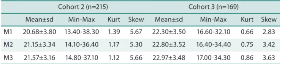
Descriptive statistics for BMI values from each cohort are shown in Table 1. Mean BMI values increased with time. It is important to highlight that kurtosis and skewness values suggest violations to normality.
Table 1. Descriptive statistics for BMI values from cohorts 2 and 3.
Cohort 2 (n=215) Cohort 3 (n=169)
Mean±sd Min-Max Kurt Skew Mean±sd Min-Max Kurt Skew M1 20.68±3.80 13.40-38.30 1.39 5.67 22.30±3.50 16.60-32.10 0.66 2.83 M2 21.15±3.34 14.10-36.40 1.17 5.30 22.80±3.52 16.40-34.40 0.75 3.42
M3 21.57±3.16 14.80-37.10 1.12 5.66 22.97±3.48 17.00-34.30 0.86 3.63
M1: First year of assessment; M2: Second year of assessment; M3: Third year of assessment; sd: standard deviation; Min: minimum; Max: maximum; Kurt: kurtosis coeicient; Skew: skewness coeicient.
Auto-correlations
An important part of tracking studies in Physical Activity Epidemiology and Physical Fitness resorts to the calculation of correlations (r) among the same variables sequentially measured in time, calculating what is known as auto-correlations16. Regardless of interpretation of r values based on formal
tests of the null hypothesis(H0:r=0), Malina16 subjectively suggested cut-of
Tracking and its applicability Souza et al.
randomly distributed; (iii) have homoscedasticity; and (iv) have bivariate or multivariate normal distributions17. In Table 1, skewness and kurtosis
suggest potential violation to normality of the BMI distributions at each age group in each cohort.
he analysis of univariate, bivariate and multivariate normality of BMI distributions at diferent time points in each cohort was performed in STATA 12. he results (not included in the text) showed violation of these assumptions. When BMI values were transformed (1/BMI), univariate normality was achieved, but violations to bivariate and multivariate nor-mality still could be found. To solve this problem, some authors suggest using Spearman correlation coeicient (less eicient than Pearson, but not sensitive to kurtoses problems in the distributions or presence of outliers17).
However, our choice was diferent as we decided to make a robust analysis suggested by Hadi18 and implemented in SYSTAT 13 in which a resampling
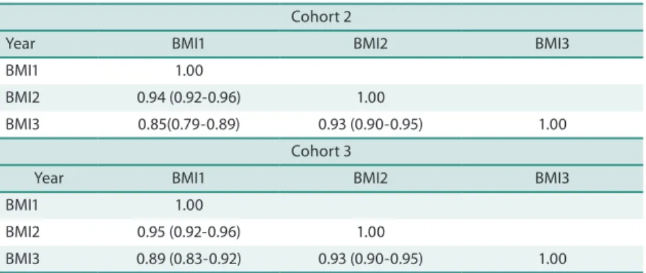
method (bootstrap) with 500 samples equal to the size of samples for each cohort was added in order to obtain standard errors to helps us in the con-struction of conidence intervals for all r values, providing a more precise view of tracking coeicients (see Table 2).
Table 2.Auto-correlations and their respective conidence intervals (CI 95%) between BMI measurements over
3 years in each cohort.
Cohort 2
Year BMI1 BMI2 BMI3
BMI1 1.00
BMI2 0.94 (0.92-0.96) 1.00
BMI3 0.85(0.79-0.89) 0.93 (0.90-0.95) 1.00
Cohort 3
Year BMI1 BMI2 BMI3
BMI1 1.00
BMI2 0.95 (0.92-0.96) 1.00
BMI3 0.89 (0.83-0.92) 0.93 (0.90-0.95) 1.00
BMI1: Body mass index-irst year of assessment; BMI2:Body mass index-second year of assessment;BMI3: Body mass index-third year of assessment.
Based on the correlational strength rubric of Malina16, there was a
strong stability of BMI in girls aged 12-14 years and 14-16 years. In addition, the width of conidence intervals is extremely low, which conirms the ac-curacy of estimates. It was also possible to verify that the auto-correlation is lower between BMI1 and BMI3 in both cohorts, which relects the higher temporal spacing between measurements. Despite the simplicity in the in-terpretation of r-values, some authors16,19 highlighted the need to consider
(i) the age of the irst observation (the lower the child’s age, the lower the correlation coeicients), and (ii) individual characteristics given the obvi-ous biological variation among subjects (maturational timing and tempo). In short, although auto-correlations are widely used in tracking studies, and the BMI values obtained in both cohorts were very high, Rogosa et al.20
(ii) the Malina16 cut-of points are arbitrary; and (iii) there is no single
correlation value to describe stability. In our example, three auto-correlations were reported, because we have three time measurements; if we had 6 time points, we would have an auto-correlation matrix with 15 values (the general formula to compute the number of possible auto-correlations is k(k-1)/2, where k=number of points in time).
Foulkes & Davis
g
9Foulkes & Davis g examined the probability that two growth curves do not intersect (cross) over time; in addition, it is based on the notion that the greater the number of pairs of individuals that maintain their relative position within a distribution over the study time frame, the greater the tracking9. he g only takes positive values, ranging from 0 to 1. he higher
the g, the lower the number of crossings among growth curves. Foulkes & Davies presented reference values for g: g<0.50 no tracking; 0.50<g<1.00 tracking is present; g= 1:00, perfect tracking9.
Foulkes & Davisg have two formulations: a simple (FD1) and a more complex version (FD2)22. he simple version does not require any a priori
deinition of the change trajectory shape (linear or nonlinear), since it is a non-parametric statistic that assumes the following: 1) the simpler the trajectory, the higher the g value ; and 2) the tracking of the extremes is much higher when compared to those who are situated close to the mean trajectory21-23. In our example, we chose the complex version (FD2), which
requires, in addition, a formal and sequential test of the better function (limited to a 4th degree polynomial) that best describes individual
trajec-tories24,25. his analysis was performed on the Longitudinal Data Analysis
program (LDA) developed by Schneiderman and Kowalski26.
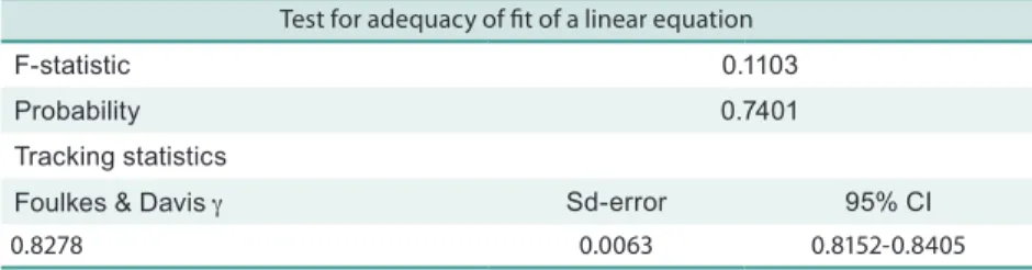
Table 3. Results of the best function that describes data and the Foulkes & Davis g statistics for cohort 2.
Test for adequacy of it of a linear equation
F-statistic 0.1103
Probability 0.7401
Tracking statistics
Foulkes & Davisg Sd-error 95% CI
0.8278 0.0063 0.8152-0.8405
g: Gamma; 95% CI: 95% Conidence Interval.
Tracking and its applicability Souza et al.
Although Foulkes & Davis g have a more complex mathematical-statis-tical structure when compared to auto-correlations and requires specialized sotware for its computation, its formulation has several advantages24,25
including: 1) collected data do not need to be equally spaced in time; 2) there is no special need for Gaussian distributions; 3) a test is available to identify the best itting model describing change; 4) it has a unique tracking statistics and is associated with 95% CI; and 5) it allows the identiication of individuals whose growth curves are more or less stable and therefore more or less predictable.
g
Statistics according to David Rogosa
10,20,27he method proposed by Rogosa20, detailed in the sotware developed with
Ghandour (TIMEPATH)10, is based on a seminal paper published with
San-ner28, as well as in his "classic" work reprinted in 199527. he sotware output
ofers the following: 1) best itting models for individual growth curves as well as group statistics; 2) values of a single individual g, and 3) population estimates with standard-errors, which allows for computations of 95% CI.
Since there is an individual g and therefore 169 g’s in cohort 3, the sotware presents relevant descriptive statistics (mean, standard deviation, minimum and maximum), and the ive-number summary: minimum, P25 (quartile 1), median (P50), P75 (quartile 3), as well as Rates R2 and g
statis-tics. It is important to highlight that individual g refers to the probability of an individual trajectory to cross other trajectories. he information provided by the sotware is very rich in order to have a detailed description of modal BMI trajectory as well as an individualized view of its stability (given by g) and change (given by Rates). Finally, tracking population estimates are presented.
Table 4. Descriptive statistics and g tracking index according to Rogosa’s suggestions (cohort 3).
Rate R2 Gamma (g)
Mean 0.336 67.829 0.835
Standard deviation 0.917 32.807 0.098
Minimum -3.450 0.000 0.411
P5 -1.450 2.420 0.613
Q1 -0.150 42.907 0.798
Median 0.450 77.997 0.839
Q3 0.900 96.430 0.899
P95 1.550 99.734 0.976
Maximum 3.100 100.000 0.994
Gamma (g) 0.852
Standard Error 0.008
P5: Percentile 5; Q1: Quartile 1; Q3: Quartile 3; P95: Percentile 95
Rogosa’s suggestions10,20,27 as well as the versatility and richness of the
TIMEPATH output are very important in order to have a detailed view of tracking, allowing researchers a more detailed examination, in modal and individual ways, of BMI trajectories over the three years.
Goldstein’s growth constancy index
11,29he Goldstein’s growth constancy index, represented as x by Furey et al.11,
is a tracking measure aimed at determining the stability and variability of individual growth (i.e., height) trajectories. According to Goldstein29,
the analysis of change patterns occurring in children and adolescents’ growth would provide insight into the detection of stable (maintenance of a relative position) or unstable growth curves (relatively high proportion of intersecting curves). Its importance in Auxology and paediatrics is evident to timely identify children or adolescents with instability in their physical growth. Goldstein29 proposed that in a random sample of individuals, an
individual whose growth curve crosses a relatively high proportion of other subjects´ curves is characterized as having a low tracking.
Goldstein29 presented two ways of estimating the growth constancy
index, i.e., tracking measures. In the irst approach, x and its conidence interval are based on a Jackknife estimator. In the second approach, the use of the intraclass correlation obtained from the analysis of variance (ANOVA) was suggested. hese two options can be formulated, as stressed by Furey et al.11, in the context of two ANOVA models29. hus, in model I or II, the
problem lies in the way the true value of each individual is formulated, its true stability and interpretation. In model I, this value is considered as an unknown (i.e., a constant), whereas in model II, it is considered as a random variable. he interpretation in the case of ANOVA I is the following: track-ing inferences are valid only for cases included in the study; in ANOVA II, the inferences are made to the population consisting of individuals from where the sample was randomly extracted. Table 5 shows examples of these analyses. In Model I, a typical ANOVA table is shown, and x is presented (its values vary from 0 to 1, and 1 is the perfect tracking). According to Furey et al.11, this index may be overestimated and may assume positive
values even when there is no evident tracking. In this case, it is necessary to consider its modiied or corrected value (x*) with a maximum value of 1, but it becomes 0 if auto-correlations are equal to 0 in successive values. he last part of model I shows point estimates as well as conidence intervals obtained by the Jackknife resampling technique. In Model II, an ANOVA table is also presented. However, tracking is expressed as an intraclass cor-relation coeicient. In addition, the 95% conidence interval is also shown11.
Tracking and its applicability Souza et al.
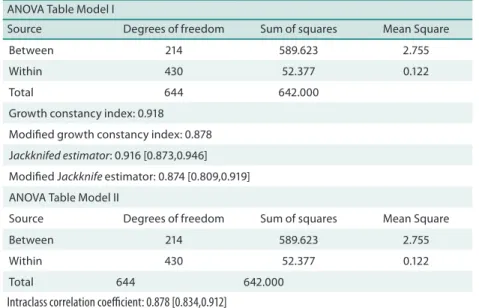
estimates and corresponding 95% CI were 0.916 (0.873, 0.946) and 0.874 (0.809, 0.919) for cohort 2; 0.939 (0.915, 0.957) and 0.909 (0.873, 0.936) for cohort 3.
Table 5. Model I and II of the Golsdstein’s growth constancy index11,29 of the BMI of girls from cohort 2.
ANOVA Table Model I
Source Degrees of freedom Sum of squares Mean Square
Between 214 589.623 2.755
Within 430 52.377 0.122
Total 644 642.000
Growth constancy index: 0.918 Modiied growth constancy index: 0.878 Jackknifed estimator: 0.916 [0.873,0.946] Modiied Jackknife estimator: 0.874 [0.809,0.919] ANOVA Table Model II
Source Degrees of freedom Sum of squares Mean Square
Between 214 589.623 2.755
Within 430 52.377 0.122
Total 644 642.000
Intraclass correlation coeicient: 0.878 [0.834,0.912]
Results of model II (generalization allowed for girls of the same popu-lation), the intraclass correlation coeicient and 95% CI was 0.878 (0.834, 0.912) for girls in cohort 2 and 0.910 (0.876, 0.935) in cohort 3. hese results show, once again, BMI stability for girls aged 12-14 years and 14-16 years. In short, the wealth of Goldstein’s suggestion11,29 can be extended to
tracking studies covering other variables without additional problems. In addition to obtaining a single tracking measure, its computation does not require equidistant observations, and Gaussian distribution is not required. One of the advantages of Goldstein propositions is the identiication of individuals with high or low separation to the mean, allowing eicient monitoring and intervention of lagged cases.
CONCLUSION
his paper presents a set of diferent tracking approaches aimed at helping a novice researcher in the ield. he importance of the tracking concept, its various statistical analysis techniques, and meaning may constitute important methodological lessons in the Physical Education and Sports Science ields, especially when dealing with longitudinal data arising from observational and/or intervention designs. Notwithstanding, the variety of statistical approaches, it may be important for researchers to become acquainted with their versatility, implementation in diferent sotware, utility and application.
auto-cor-explored, a more individualized view of each subject becomes more evident, allowing identifying adolescents who may require individual care and more eicient interventions from Physical Education teachers or paediatricians.
Acknowledgment
To CAPES Foundation, the Ministry of Education of Brazil, Brasília-DF, for the scholarship granted to Professor Michele Caroline de Souza.
REFERENCES
1. Gonzalez A, Boyle MH, Georgiades K, Duncan L, Atkinson LR, MacMillan HL. Childhood and family inluences on body mass index in early adulthood: indings from the Ontario Child Health Study. BMC Public Health 2012;12:755.
2. Bahia L, Coutinho ES, Barufaldi LA, Abreu Gde A, Malhao TA, de Souza CP, et al. he costs of overweight and obesity-related diseases in the Brazilian public health system: cross-sectional study. BMC Public Health 2012;12:440.
3. Bayer O, Kruger H, von Kries R, Toschke AM. Factors associated with tracking of BMI: a meta-regression analysis on BMI tracking. Obesity 2011;19(5):1069-76.
4. Lloyd-Jones D, Adams RJ, Brown TM, Carnethon M, Dai S, De Simone G, et al. Executive summary: heart disease and stroke statistics--2010 update: a report from the American Heart Association. Circulation 2010;121(7):948-54.
5. Kowalski CJ, Schneiderman ED. Tracking: Concepts, Methods and Tools. Int J Anthropol 1992;7(4):33-50.
6. Freitas D, Beunen G, Maia J, Claessens A, homis M, Marques A, et al. Tracking of fatness during childhood, adolescence and young adulthood: a 7-year follow-up study in Madeira Island, Portugal. Ann Hum Biol 2012;39(1):59-67.
7. Da Silva SP, Beunen G, Prista A, Maia J. Short-term tracking of performance and health-related physical itness in girls: the Healthy Growth in Cariri Study. J Sports Sci 2013;31(1):104-13.
8. Malina RM. Tracking of physical activity and physical itness across the lifespan. Res Q Exerc Sport 1996;67(3 Suppl):S48-57.
9. Foulkes MA, Davis LE. An index of tracking for longitudinal data. Biometrics 1981;37:439-46.
10. Rogosa D, Ghandour G. TIMEPATH: Statistical analysis of individual trajectories. CA S, editor: Stanford University; 1989.
11. Furey A, Kowalski C, Schneiderman E, Willis S. GTRACK: A PC program for computing Goldstein’s growth constancy index and an alternative measure of tracking. Int J Bio-Med Comput 1994;36(1):311-8.
12. Guo SS, Chumlea WC. Tracking of body mass index in children in relation to overweight in adulthood. Am J Clin Nutr 1999;70(1):145S-8S.
13. Malina RM, Katzmarzyk PT. Validity of the body mass index as an indicator of the risk and presence of overweight in adolescents. Am J Clin Nutr 1999;70(1):131S-6S.
14. Malina R, Bouchard C, Bar-Or O. Growth, maturation and physical activity. Champaign, editor: Human Kinetics; 2004.
15. Maia J, Silva R, Seabra A, Lopes VP. A importância do estudo do tracking (es-tabilidade e previsão) em delineamentos longitudinais: um estudo aplicado à epidemiologia da actividade física e à performance desportivo-motora. Rev Port Cien Desp 2002;2(4):41-56.
16. Malina RM. Adherence to physical activity from childhood to adulthood : a per-spective from tracking studies. Quest 2001;53(1):346-55.
Tracking and its applicability Souza et al.
Corresponding author
Michele Caroline de Souza CIFI2D, Laboratório de Cineantropometria e Estatística Aplicada.
Faculdade de Desporto, Universidade do Porto.
Rua Dr. Plácido Costa, 91. 4200-450, Porto, Portugal. E-mail: [email protected]
18. Hadi A. A modiication of a method for the detection of outliers in multivariate samples. J R Statist Soc B 1994;Series (B), 56.
19. Glenmark B, Hedberg G, Jansson E. Prediction of physical activity level in adult-hood by physical characteristics, physical performance and physical activity in adolescence: an 11-year follow-up study. Eur J Appl Physiol Occup Physiol 1994;69(6):530-8.
20. Rogosa D, Floden R, Willet J. Assessing the stability of teacher behavior. J Educ Psychol 1984;76(1):1000-27.
21. Twisk JW, Kemper HC, Mellenbergh GJ. Mathematical and analytical aspects of tracking. Epidemiol Rev 1994;16(2):165-83.
22. Schneiderman E, Kowalski C, Ten Have T. A GAUSS prgram for computing an index of tracking from longitudinal observations. Am J Hum Biol 1990;2(1):475-90.
23. Maia J, Garganta R, Seabra A, Lopes VP, Silva S, Meira Júniro C. Explorando a noção e signiicado do tracking. Um percurso didático para investigadores. Psico-logiapt 2007.
24. Schneiderman E, Willis S, Kowalski C, Ten Have T. A GAUUS program for comput-ing the Foulkes-Davis Trackcomput-ing Index for polynomial growth curves. Int J Bio-Med Comput 1993;32(1):35-43.
25. Schneiderman ED, Kowalski CJ. Analysis of longitudinal data in craniofacial re-search: some strategies. Crit Rev Oral Biol Med 1994;5(3-4):187-202.
26. Schneiderman E, Kowalski C. LDA. Sotware system for longitudinal data analysis. Version 3.2. . Texas: Baylor College of Dentistry; 1993.
27. Rogosa D. Myths and methods: Myths about longitudinal research plus supplemen-. tal questions. In: Gottman J, editor. he analysis of change. New Jersey: Lawrence Erlbaum Associates; 1995. p. 3-65.
28. Rogosa D, Saner H. Longitudinal data analysis examples with random coeicient models. J Educ Behav Statist 1995;20.