TIME-SEGMENTED FREQUENCY-DOMAIN ANALYSIS FOR NON-LINEAR MULTI-DEGREE-OF-FREEDOM STRUCTURAL SYSTEMS

Journal of Sound and ibration(2000) (3), 457 475

doi:10.1006/jsvi.2000.3066, available online at http://www.idealibrary.com on

TIME-SEGMENTED FREQUENCY-DOMAIN ANALYSIS

FOR NON-LINEAR MULTI-DEGREE-OF-FREEDOM

STRUCTURAL SYSTEMS

W. J. MANSUR ANDJ. A. M. CARRER

Department of Civil Engineering,COPPE/Federal;_{niversity of Rio de Janeiro,CEP21945-970,} Rio de Janeiro C.P. 68506,RJ,Brazil.E-mail:webe@coc.ufrj.br

W. G. FERREIRA

¹echnological Center,Federal;_{niversity of Espirito Santo,}<_{itoria,Brazil} A. M. CLARET DEGOUVEIA

School of Mines,Federal;_{niversity of Ouro Preto,Ouro Preto,Brazil}

AND

F. VENANCIO-FILHO

Department of Applied Mechanics and Structures,Federal;_{niversity of Rio de Janeiro,} Rio de Janeiro,Brazil

(Received30August1999,and in,nal form24April2000)

This paper presents a new frequency-domain method to analyze physically non-linear structural systems having non-proportional damping. Single- and multi-degree-of-freedom (d.o.f.) systems subjected to time-dependent excitations are considered. A procedure to consider initial conditions, required by the methodology described, is discussed. The algorithm described here employs a time-segmented procedure in modal co-ordinates in the frequency domain; solution in each time-segment being obtained by an iterative process. The proposed methodology is validated by three examples. The procedure presented here can be employed as well to analyze structural systems with viscous and hysteretic damping or else with frequency-dependent damping properties.

(2000 Academic Press

1. INTRODUCTION

Dynamic non-linear analyses are usually performed in the time-domain by direct integration of the equations of motion in physical co-ordinates. The so-called mode superposition method has also been used as an alternative time-domain procedure, where modal co-ordinates are employed instead of the physical ones. However, when the structural system has hysteretic damping or frequency-dependent damping characteristics, the analysis in frequency domain is more adequate.

In recent years, a number of procedures have been presented for non-linear analyses in the frequency domain. Kawamoto [1] proposed a hybrid time-frequency method where the original system is replaced by a pseudo-linear system; the equations of motion being solved in the frequency domain, and the non-linear contribution being dealt with in the time-domain through the pseudo-force method. Aprile et al. [2] generalized

Kawamoto's procedure making it possible to consider hysteretic and frequency-dependent damping.

Itoh [3] presented a frequency-domain procedure to obtain responses of systems with non-proportional damping where he makes use of a complex modal basis to uncouple the equations of motion. The "nal algorithm employs only real algebra, and does not take advantage of some characteristics of the classical mode superposition method.

Chen and Taylor [4] proposed uncoupling the dynamic equilibrium equations for systems with non-proportional damping, through a basis composed by Ritz vectors instead of the complex modal basis. Chang and Mohraz [5] used the mode superposition method to deal with physically non-linear structural systems with non-proportional damping; they established an iterative procedure through Taylor series expansions.

Claret and Venancio-Filho [6] considered non-proportional damping via the pseudo-force concept. The pseudo-force formulation led to an iterative process, which was solved in the time-domain via Duhamel integral. The convergence of the iterative process was quite good. Jangid and Datta [7] employed the same procedure as Claret and Venancio-Filho; however the iterative process was performed in the frequency domain.

The present work is concerned with a discussion aiming at generalizing existing frequency-domain procedures for non-linear structural systems with non-proportional damping. A new and quite general methodology to consider physical non-linearities is presented, making it possible to consider structural damping. The solution of either linear or non-linear single-degree-of-freedom (s.d.o.f.) systems is obtained by the matrix formulation presented by Venancio-Filho and Claret [8], namely the implicit Fourier transform (ImFT ). It is important to mention that concerning the non-linear formulation initial conditions are considered as described by Ferreiraet al. [9] and that the procedure presented in that paper is herein generalized to consider multi-degree-of-freedom systems. In order to obtain the time-history of the response for non-linear s.d.o.f. or m.d.o.f. systems with non-proportional damping, a time segmentation technique is employed over modal co-ordinates. The coe$cients responsible for coupling are considered as pseudo-forces, thus an iterative procedure naturally arises.

2. LINEAR SINGLE-DEGREE-OF-FREEDOM SYSTEMS

The equation of motion for an s.d.o.f. system with viscous damping is given by

mvK(t)#cvR(t)#kv(t)"p(t), (1)

wherem,candkare, respectively, mass, damping and sti!ness coe$cients, andvis the mass displacement.

The time-domain solution of equation (1) can be obtained through the following inverse discrete Fourier transform (iDFT) formula:

v(t

n)"

DuN

2n N~1₊

m/0

H(uN

m)P(uNm)emn(*(2n@N)) (2)

whereP(uN_m) is the discrete Fourier transform (DFT) ofp(t), i.e.,

P(uN_m)"DtN~1+ n/0

p(t

iis the complex unit,Nis the number of sampling points,t

n"nDt, are the discrete times, Dt"¹

p/N is the time interval in which the sampling time ¹p is subdivided. ¹p is also referred to as extended period and uN_m"mDuN are the discrete frequencies, where DuN"2p/¹

p. H(uN m) is the complex frequency response function (CFRF) at the discrete frequencyuN_m, i.e.,

H(uN_m)"

G

1

!uN2_mm#k#iuN _mc for m)N/2,

conjugate[(H(uN_N~m))] for m'N/2.

(4)

It is important to notice that the spectrum ofv(t),

<(uN

m)"H(uN m)P(uN m), (5)

is available to the engineer (see equation (2)) when the standard DFT algorithm described above is employed.

The linear viscous damping model (see equation (1)) is currently adopted because it leads to a convenient solution of the equation of motion and it can be adjusted to yield reasonable results as long as damping is not too high. However, its use in structural dynamics is at least conceptually incorrect as viscous-damping modelling leads to frequency-dependent energy dissipation for harmonic motions, i.e., the damped system behaves in a way which lacks experimental support. Thus, in what concerns structural damping, whenever possible one should use a model whose energy dissipation is not frequency dependent. Such a model is the so-called hysteretic damping model, for which the CFRF for the s.d.o.f. system can be expressed as

H(uN_m)" 1 !uN 2

mm#k(1#ij)

, (6)

j"2mbeing the hysteretic damping factor andmbeing the damping ratio [10].

The discrete time-history of displacement obtained by the DFT procedure as shown by equations (2) and (3), can be alternatively obtained by a unique matrix operation

v"1

Nep, (7)

wherevis a vector describing the mass displacement time-history whose entriesv

nare equal to v(t

n), p is the discrete loading vector whose entries are pn"p(tn). As all operations required to perform the DFT and the iDFT are implicitly considered by matrixe, it is called the implicit Fourier transform matrix. The following matrix product obtains the entries of matrixe:

e"EHE*, (8)

where E*carries out in matrix form the DFT operation indicated by equation (3), i.e., P"DtE*p,Pbeing a vector whose entries areP

n"P(uNm).E*entries are given by

E*

m`1,n`1"e~mn(*(2n@N)) (9) E carries out in matrix form the iDFT operation indicated by equation (2), i.e., v"(DuN /2n)EHP, H being a diagonal matrix whose entries are H

Eentries are given by

E

m`1,n`1"emn(*(2n@N)), (10) i.e.,E

m`1,n`1"conj(E*m`1,n`1).

The discrete time-history of velocities can be computed as indicated by Ferreira [11] and Ferreiraet al. [9].

Now, one of the advantages of using the implicit Fourier transform (ImFT) algorithm described above (see equation (7)) appears at full extent. If the number of Fourier coe$cients is large enough to yield accurate time response forvas expressed by equation (7) and the extended period is large enough, causality should be obeyed, i.e., a discrete value of

p(t

j) should not contribute to a discrete value of v(ti) whenever j'i. Thus, if one is interested only in the"rstSterms of the response, only the coe$cientse

ijsuch thati)S,

i'j, need to be considered. Such a reduced e (S]S) lower triangular matrix can be generated by the complete H (N]N) matrix and by reduced E (S]N) and E* (N]S) matrices. The causality property described above will prove to be very useful in the scheme for non-linear analysis presented in this paper where a lower triangulare(S]S) matrix together with reduced (S]1) p and v vectors are considered rather than a complete e (N]N) matrix and complete (N]1) p and v vectors. One must also notice that the

e

ijcoe$cients have a number of properties as described by Ferreira [11] which if taken into consideration lead to substantial savings in the assemblage of theematrix. An important characteristic of matrix e which must be observed is that e is a Toeplitz matrix, i.e.,

e

i`k,j`k"ei,j). Thus, only its"rst column has to be calculated.

3. INITIAL CONDITIONS

Aiming at performing a time-segmented non-linear analysis, where displacement and velocity at the end of one segment are used as initial conditions for the subsequent segment, a procedure to include initial displacement and velocity is discussed next.

The time response due to an initial displacement v

0 can be obtained by adding to a constant in time displacementv

0, the e!ect of a force!f0:

v"1

Ne(!f01)#v01, (11)

where1is a vector of order (S]1), whose elements are equal to unity andf

0is the static force on the spring due to the displacementv

0. If the analysis is linear elastic, thenf0"k0v0, if it is non-linear,f

0must be obtained from the load]displacement diagram for the spring. The response corresponding to an initial velocityvR₀is the same as that due to an impulse of intensitymvR₀, which can be obtained from

v(t)"mvR₀h(t), (12)

whereh(t) is the unit-impulse response function, i.e., it is the response of the s.d.o.f. system to a unit impulse. From equation (12) one can obtain the discrete time-history displacement vector [9,11] corresponding to an initial velocityvR₀,

v" 1

NDtmvR0ed, (13)

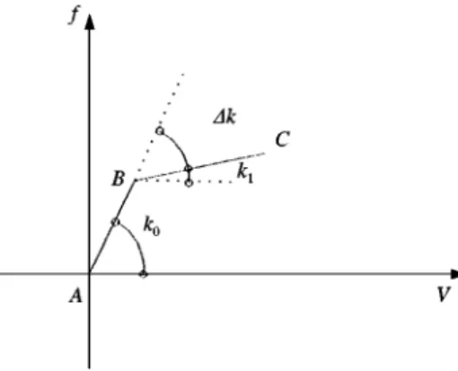
Figure 1. Bilinear force-de#ection diagram.

When both initial displacement and velocity are considered, one "nally arrives at the following expression, which can be used in a time-segmented analysis:

v"1

Ne

A

Dt d

B

4. SINGLE-DEGREE-OF-FREEDOM NON-LINEAR SYSTEMS

Consider a non-linear s.d.o.f. system, whose spring force}de#ection relation follows the bilinear law shown in Figure 1.

During the time-marching process, the equilibrium equation may correspond either to segmentA}BorB}C. When the time-marching process starts, the analysis is carried out within segment A}B with null initial conditions. The equation of motion then reads

mvK#cvR#k

0v"p (15)

and the time response can be obtained from

v"1

Nep (16)

For segmentB}C, the equation of motion reads [12]

mvK

n#cvRn#k1vn"pn!f0, (17)

wherev

n"v!v0,vis the total displacement within segmentB}Cat timet, andv0is the displacement at the end of segment A}B. f

0 (f0"k0v0) is the external reaction force resulting from a static analysis when the mass is subjected to the displacementv

0. Figure 1 shows that

k

1"k0!Dk. (18)

Considering equations (17) and (18) the following expression can be derived:

mvK

Figure 2. Bilinear force}de#ection diagram and time-history of the mass displacement.

m,candk

0on the left hand side (l.h.s.) of equation (19) are the same as for the linear segment

A}B(see equation (15)) and the termDkv

nwhich corresponds to the spring sti!ness change, is in fact considered as a pseudo-force, as it now appears on the right hand side (r.h.s.) of equation (19). The iterative procedure employed to solve equation (19) can be described by equation (20), which represents the equation of motion for iterationk:

mvK(k)_n #cvR(k)_n #k

0v(k)n "pn#Dkv(k~1)n !f0. (20) The displacement time-history can then be obtained from

v_(k)"v_(k)

n #v01, v(k)n " 1

Ne

A

Dt d#Dkv(k~)n

B

where the contribution of initial velocity has also been included. It should be noticed that the implicit Fourier transform matrix e is that of segment A}B, i.e., it need not be recalculated.

The iterative process is stopped when

K

max!v(k~1)max

v_(k)

max

K

)e, (22)

ebeing a given tolerance.

Figure 2 illustrates a typical bilinear force}de#ection diagram and the mass displacement time-history, corresponding to a segmented analysis with"ve segments: O}A;A}B; B}C,

C}D,D}. The end of the analysis shown in Figure 2 is on the"fth segment where the mass oscillates until it stops. The initial conditions are shown in Table 1.

5. MULTI-DEGREE-OF-FREEDOM LINEAR SYSTEMS

The equation of motion for a viscously damped m.d.o.f. system can be written as

mvK(t)#cv5(t)#kv(t)"p(t), (23)

wherem,candk are, respectively, mass, damping and sti!ness matrices. Equation (23) can be transformed to modal co-ordinatesY(t) as

TABLE1

Segmentation analysis sequence and initial conditions for each segment indicated in Figure2

Segment Initial conditions

O}A f

0"0 v0"0 vR0"0

A}B f

0"fA v0"vA vR0"vRA

B}C f

0"fB v0"vB vR0"vRB

C}D f

0"fC v0"vC vR0"vRC

D} f

0"fD v0"vD vR0"vRD

wherev(t)"U_{Y(t) andP(t)}"U_Tp(t).U_{is the modal matrix normalized with respect to the}

mass matrix, thusIin equation (24) is a diagonal unitary mass matrix,K_{is diagonal and}

Cwill be diagonal ifcis proportional, i.e.,c"a

0m#a1k.

When the damping matrixcis proportional the system of equations given by equation (24) is uncoupled and the solution for a modal co-ordinateY

j, when initial conditions are null, can be obtained from

Y j"

1

NejPj, (25)

where

e

j"EHjE*. (26)

H

jis a diagonal matrix whose diagonal coe$cients (Hj)m`1,m`1are given by

H

j(uNm)"1/[!uN 2m#iuNmCjj#(1#ij)u2j] (27) and u

j is the jth natural frequency obtained from the solution of the equation [k!u₂m]v"0.

The time response for the physical co-ordinates can be computed from

v(t)"U_{Y(t), (28)}

6. NON-LINEAR MULTI-DEGREE-OF-FREEDOM SYSTEMS WITH PROPORTIONAL DAMPING

The procedure followed for non-linear m.d.o.f. systems is similar to that explained previously for s.d.o.f. systems. The solution process starts on the"rst segment (linear) for which the procedure indicated by equations (23)}(28) holds.

When the non-linear term responsible for the change in sti!ness is considered as pseudo-force, as before, an iterative process arises, and the equilibrium equation for thekth iteration reads

mvK(k)_n #cv5_n(k)#k₀v(k)_n "p

n#Dkv(k~1)n !f0, (29) wherek

0is the sti!ness matrix corresponding to the"rst segment. As the matrices on the l.h.s. of equation (29) are the same as those shown in equation (23), withk

(29). However, the eigenvalues of the"rst segment are not orthogonal to the incremental matrix Dk, consequently the modal incremental matrix K

N"UTDkU will have coupled modal coe$cients.

Thus, the modal displacement time-history corresponding to equation (29) can be found through the following iterative expressions:

Y(k)

j "Y(k)nj#>0j1,

Y(k) nj"

1

Nej

A

>Q j

Dtd#

NGL + p/1

K

NjpY(k~1)np

B

where F

0j is the modal reaction which appears on the generalized mass j when the mechanical system is subjected to a static displacement"eld corresponding to the initial displacement of the current segment and>Q

0jis the corresponding initial modal velocity. In order to further clarify howF

0jis evaluated in a numerical algorithm such as that described in this paper, consider a m.d.o.f. system having only one non-linear spring whose displacement}de#ection curve is shown in Figure 2. Concerning the discussion that follows it is instructive to label segmentsO}A,B}CandD}Eas linear and to label segmentsA}B

andC}Das non-linear.

In order to compute the time response for the C}D segment, the displacement and velocities of pointCof segmentB}Care taken as initial conditions for segmentC}D. Thus,

F

0jis given by

F

0j"Faj#K0jD>0j (31)

whereK

0jis thejth diagonal coe$cient of the modal sti!ness matrixK0"UTk0UandD>0j is the incremental modal displacement of the generalized massjat the end of the segment

B}C.K

0jD>0jis an incremental modal static linear elastic force on the generalized mass

jandF_ajrepresents static force contributions due to previous segments.

As the procedure is segmented, the next step consists in"nding the response for segment

D}E. The"nal conditions of segmentC}Dare now the initial conditions for segmentD}E. In this case,F

0+for segmentD}Ereads

F

0j"Faj#uTjk1vn (32)

whereu

+is thejth eigenvector andvnis the incremental displacement vector of the masses at the end of the non-linear segment C}D, expressed in physical co-ordinates. Therefore, uT

jk1vnis the incremental modal static force at the generalized massjthat corresponds to the end of the segment C}D, and F_aj is equal to F

0j given by equation (31). Thus, the following general expression can be written:

Fa"+

a [K

0jD>0j]a#+ b

[uTk

1vn]b, (33)

where the summations account for contributions of previous steps, both linear (+

a[K0jD>0j]a) and non-linear (+b[uTk1vn]b).

7. NON-LINEAR MULTI-DEGREE-OF-FREEDOM SYSTEMS WITH NON-PROPORTIONAL DAMPING

used and the coe$cients of the modal damping matrix responsible for mode coupling are transferred to the r.h.s. of the modal system of equations. In order to accomplish this task the modal damping matrixC"UT_{cU must be written as}

C"C

D#CF, (34)

whereC

Dis a diagonal matrix whose coe$cients are given by

C

Dnn"uTncun"2mnun (35)

andC

Fis a matrix whose diagonal coe$cients are null with the non-diagonal terms given by

C

Fnp"uTncup (CFnp"0 if n"p). (36) The term which accounts for pseudo-forces due to non-proportional damping can be obtained by following a procedure similar to that developed when non-linearities were considered. When non-linear behaviour is considered together with non-proportional damping, the following equation for thekth iteration can be written

Y(k)

j "Y(k)nj#>0j1,

Y(k) nj"

1

Nej

A

>Q j

Dtd#

NGL + p/1

K

NjpY(k~1)np ! NGL

+ p/1

C

FjpY0 (k~1)np

B

8. NUMERICAL EXAMPLES

8.1. PRELIMINARY REMARKS

In order to carry out a numerical analysis one hasa priorito make a decision about the values of DFT parameters which lead to accurate numerical results. Some guidelines may be recommended; however, an optimal choice of such parameters can only be achieved if one has experience in the problem being analyzed.

8.1.1. Extended period¹

p

The period either for linear analyses or for each segment of non-linear analysis must be large enough to prevent a periodic behaviour of the time-history of displacements. Aseis a lower triangular matrix, the extended period¹

pis not related to time duration of external loads, rather it must be such that the"rst column of matrixeis accurately computed (note thateis a Toeplitz matrix). In fact,¹

pdepends only onm,candk, and must be such that

g(¹

p) is small,g(t) being the unit impulse response function which for an s.d.o.f. system is given by

g(t)" 1

uJ1!m₂e~umtsin(utJ1

!m₂). (38)

Given a tolerancea, ¹

pcan be estimated from

or

¹

p'a ln(10)

mu (40)

wheremis the damping ratio anduis the natural frequency.

The authors have obtained accurate results fora"2 and recommend 2)a)4.

8.1.2. Number of sampling points N

As is usual in DFT analysis the number of sampling points must preventaliasing[10,13], i.e., the sampling intervalDtmust be small enough so that

1

2Dt'fN, (41)

wheref

Nis the Nyquist frequency. The sampling interval isDt"¹p/(N!1).

8.1.3. ¹he parameter S

This parameter only indicates the number of time points at which the response is to be computed. As such it has no in#uence either on accuracy or on stability of the algorithm. However,Shas great in#uence on the cost of the analysis mainly for non-linear structural systems.Sbeing too small introduces unnecessary segments, whereas large values ofSlead to unnecessary computations of the response beyond a segment.

8.1.4. ¹oleranceeof the pseudo-force iterative process

In all examples analyzed here the authors have adoptede"1%.

8.1.5. ¹ime-domain analyses

Figure 3. Single-degree-of-freedom shear building: (a) properties; (b) bilinear sti!ness coe$cient.

8.2. EXAMPLE1

The s.d.o.f. system shown in Figure 3(a) has mass equal to 17)5 t and a viscous damping

coe$cient equal to 21 kN s/m. The spring sti!ness coe$cient is bilinear as shown in Figure 3(b). The natural frequency is 7)07 rad/s and the damping ratio is 8)5%.

The following parameters, related to the implicit Fourier transform algorithm and to the iterative pseudo-force process, were adopted:N"2000,Dt"0)0125,S"120 ande"1%.

For the time-domain analysis,Dt"0)012.

In the non-linear analysis, one may have to change from the current segment to the subsequent one (see Figure 2) at discrete time values lower thanSDt(S"120), in which case the remaining terms of the time response history are not considered.

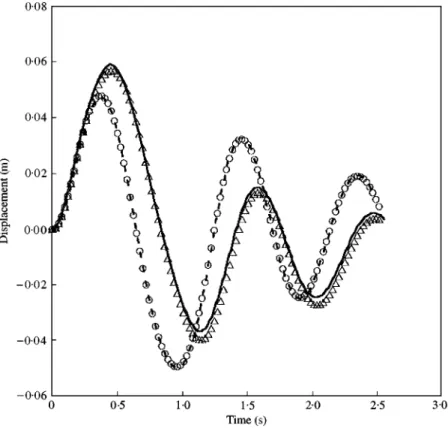
In the"rst analysis the system is subjected to the loading time-history shown in Figure 4. Linear and non-linear ImFT and Newmark responses depicted in Figure 5 agree quite well. Concerning the non-linear analysis, the spring works linearly under tension at the initial stage, reaches later a non-linear phase, subsequently enters into a compressive linear phase, returns to the non-linear phase and"nally oscillates linearly until motion stops. Thus, at rest, the spring will have a residual strain (negative in the present analysis).

In order to check the robustness of the ImFT approach, another analysis was carried out where the s.d.o.f. system shown in Figure 3 was excited by a base motion whose input acceleration, depicted in Figure 6, corresponds to the"rst 4 s of the&&El Centro''earthquake. The time-domain and ImFT results shown in Figure 7 agree quite well. For these analyses,Dt"0)0125 s. It should be observed that in this analysis the system crosses many

times the non-linear threshold.

8.3. EXAMPLE 2

The shear building depicted in Figure 8 is submitted to &&El Centro''earthquake base acceleration. The top-#oor movement is partially restricted by a discrete viscous damper whose damping constantcis equal to 3)5 MN s/m. This shear building has been analyzed

previously by Clough and Penzien [10], who computed the eigenvalues of the correspondent undamped problem.

Three di!erent situations were simulated as described next. In the "rst analysis, the discrete viscous damper was removed and Rayleigh damping was considered for the structure [10], i.e., c"a

Figure 4. Loading time-history: example 1,"rst analysis.

Figure 5. ImFT and Newmark time responses for the s.d.o.f. system subjected to the load depicted in Figure 4:

} } } }, linear analysis, ImFT;s, linear analysis, Newmark;**, non-linear analysis, ImFT;n, non-linear analysis,

Figure 6. Base acceleration of&&El Centro''earthquake.

Figure 8. Three-degree-of-freedom shear building.

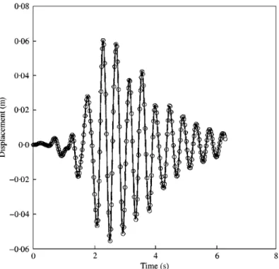
Figure 9. Displacement time-history of the top#oor of the shear building depicted in Figure 8 for proportional Rayleigh damping:**, ImFT;s_{, Newmark.}

proportional, the analysis is not iterative. Time-histories of the top #oor obtained with Newmark and ImFT algorithms, depicted in Figure 9, agree quite well.

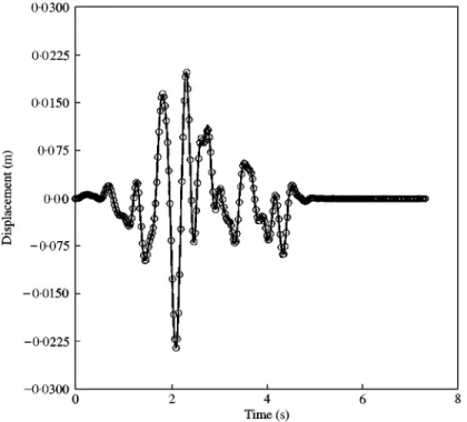
Figure 10 shows the time-history of the top-#oor displacement of the shear building as shown in Figure 8, i.e., the discrete damper is included in this analysis. Thus, the damping matrixcis non-proportional, the modal damping matrix being given by

C"

2)18 !1)65 0)55 !1)65 1)89 !0)47

Figure 10. Displacement time-history of the top#oor of the shear building depicted in Figure 8 for non-proportional damping:**, ImFT;s, Newmark.

The modal system is coupled, as the o!-diagonal coe$cients of theCmatrix shown above are not null. The pseudo-force method required four iterations to achieve convergence. Results obtained with the frequency-domain approach (ImFT), forN"1000, and with the Newmark scheme are identical.

A last analysis concerning this three-storey shear building was carried out where the discrete damper was included and hysteretic rather than Rayleigh damping was considered for the structure, the damping ratio being m"5%. The time-history of the top-#oor displacement due to the ImFT approach, using Rayleigh and hysteretic damping for the structure, is shown in Figure 11. Results, once again, agree quite well. For all analyses corresponding to this example,Dt"0)0125 s.

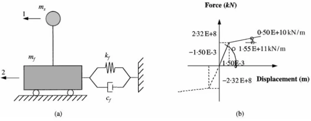
8.4. EXAMPLE 3

The 2 d.o.f. system shown in Figure 12(a) is a simpli"ed model of the structure of a nuclear reactor containment. The masses of the foundationm

fand of the structuremsare, respectively 108 and 3]107kg. The sti!ness coe$cient of the structure is

k

4"6]1010N/m. The soil behaviour is non-linear, as shown by the load}de#ection curve depicted in Figure 12(b). The system is submitted to a horizontal impact load, whose time-history is depicted in Figure 13. The damping coe$cient of the soil computed according to Richartet al. [15] is 3)79]109Ns/m. Natural frequencies corresponding to

modes 1 and 2 are, respectively, equal to 31)26 and 56)33 rad/s and the corresponding

Figure 11. Displacement time-history, obtained with the ImFT, of the top#oor of the shear building depicted in Figure 8 for non-proportional damping:**, Rayleigh damping for the structure;h, hysteretic damping for the structure.

Figure 12. Two-degree-of-freedom nuclear reactor model: (a) 2 d.o.f. system, (b) bilinear sti!ness coe$cient of the soil.

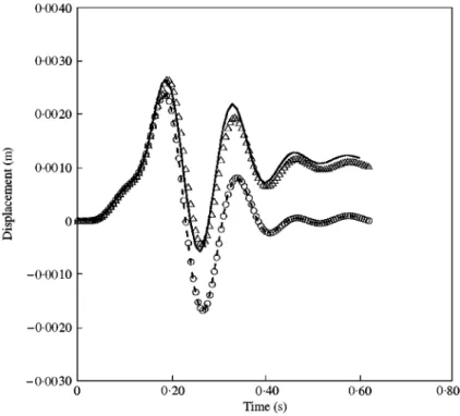
In this example the following parameters related to the implicit Fourier transform algorithm and to the iterative pseudo-force process were adopted:N"1024, Dt"0)01 s,

S"60 ande"1%.

The time-histories of the foundation displacement corresponding to Newmark (Dt"0)005 s) and ImFT algorithms are depicted in Figure 14, considering the soil

Figure 13. Impact over massm

sfor the nuclear reactor model.

non-linear with non-proportional damping. Results of time-domain and ImFT algorithms agree quite well, giving residual displacements quite close. The overall computer time for the ImFT procedure was equal to 1 s and, for the Newmark scheme, was lower than 1 s.

9. CONCLUSIONS

This work presented a new robust frequency-domain formulation, which can be used

to "nd time responses of either linear or non-linear structural systems, having

non-proportional damping characteristics.

Time-history of displacement for 1 d.o.f. systems was obtained via the matrix formulation of the discrete Fourier transform, denoted here by implicit Fourier transform (ImFT). One important property of the ImFT matrixe, the causality property, has been discussed here. It was shown that one need not consider the (N]N) terms ofewhen only the"rstS(S(N) terms of the time response history are required, i.e., a reduced lower triangulare(S]S) implicit discrete Fourier matrix can be considered, leading to substantial computer time savings.

In the procedure presented here for linear m.d.o.f. systems the mode superposition method was employed. The "nal system is uncoupled and the same frequency domain algorithm used for the 1 d.o.f. system could be employed. When the system is non-linear, with non-proportional damping, the system of equations in modal co-ordinates is not uncoupled any more. In this case, terms responsible for coupling are transferred to the r.h.s. of the system of equations, being considered as pseudo-forces. An iterative procedure arises, in which the l.h.s. of the"nal system of equations is uncoupled, and thus the modal matrix needs to be computed only once.

The pseudo-force method together with the correct consideration of initial conditions for m.d.o.f. systems led to a correct modelling in the frequency domain of the three examples discussed here; ImFT results were quite close to those arising from a time-domain procedure based on the Newmark scheme.

It is important to notice that when CPU computer time is concerned, time-domain approaches (e.g., Newmark, Wilsonh, central di!erences, etc. [14, 16]) are cheaper in many applications. However, time- and frequency-domain approaches are not meant to be competitive, rather they are complementary to one another. Time-domain procedures do not apply when dynamic properties have to be de"ned in the frequency-domain, as illustrated by the third analysis of the second example (see Figure 11) where hysteretic damping was considered for the structure. Naturally, for the range of problems to which time- and frequency-domain approaches apply equally, one will choose the cheapest one. In fact, computer time is critical when the number of the d.o.f. is too large, otherwise computer cost is not relevant.

As a "nal remark, it should be observed that ImFT computational costs could be

substantially reduced if modal truncation procedures are employed.

REFERENCES

1. J. D. KAWAMOTO1983Research Report R83-5,MI¹,Dept.of Civil Eng. Solution of nonlinear dynamic structural systems by a hybrid frequency-time domain approach.

2. A. APRILE, A. BENEDETTI and T. TROMBETTI 1994 Earthquake Engineering and Structural Dynamics3, 363}388. On non-linear dynamic analysis in the frequency domain.

4. H. CHENand R. L. TAYLOR1987 Numerical Methods in Engineering¹heory and Applications

(N;_{ME¹A87) t5/1} 2, 1}10. Properties and solutions of eigensystems of non-proportionally damped linear dynamic systems.

5. C. J. CHANGand B. MOHRAZ1990Computers and Structures36, 1067}1080. Modal analysis of non-linear systems with classical and non-classical damping.

6. A. M. CLARETand F. VENANCIO-FILHO1991Earthquake Engineering and Structural Dynamics 20, 303}315. A modal superposition pseudo-force method for dynamic analysis of structural systems with non-proportional damping.

7. R. S. JANGIDand T. K. DATTA1993Earthquake Engineering and Structural Dynamics22, 723}735. Spectral analysis of systems with non-classical damping using classical mode superposition technique.

8. F. VENANCIO-FILHOand A. M. CLARET1992 Computers and Structures42, 853}855. Matrix formulation of the dynamic analysis of SDOF in frequency domain.

9. W. G. FERREIRA, A. M. CLARET, and F. VENANCIO-FILHO1997Ibero-¸atin American Congress of Computational Methods in Engineering(XVIIICI¸AMCE)2, 815}820. The treatment of initial conditions in frequency-domain dynamic analysis.

10. R. W. CLOUGHand J. PENZIEN1993Dynamics of Structures. New York: McGraw-Hill, second edition.

11. W. G. FERREIRA1998.D.Sc.¹hesis(in Portuguese),COPPE,Federal;_{niversity of Rio de Janeiro,} Brazil. Non-linear dynamic analysis of structural systems with non-proportional damping in the frequency domain.

12. W. WEAVER, S. P. TIMOSHENKOand D. H. YOUNG1989<_{ibration Problems in Engineering. New} York: John Wiley and Sons,"fth edition.

13. M. PAZ1997Structural Dynamics2¹heory and Computations. New York: Chapman and Hall, fourth edition.

14. W. WEAVERJR. and P. R. JOHNSTON1987Structural Dynamics by Finite Elements. Englewood Cli!s, NJ: Prentice-Hall.

15. F. E. RICHARTJR, R. D. WOODSand J. R. HALLJR. 1970<_{ibrations of Soils and Foundations.} Englewood Cli!s, NJ: Prentice-Hall.