The Numerical Computation of Rational Structures and Asymptotic Standard Deviations in Causal Time Series Data

(1)

ISSN 1549-3644

Corresponding Author: Concepción González-Concepción, Department of Applied Economics, Faculty of Economics Science and Business Administration, University of La Laguna, Campus of Guajara, s/n, 38701, La Laguna, Tenerife, Canary Islands, Spain Tel: (34) 922 317029-25-26 Fax: (34) 922 317204

215

The Numerical Computation of Rational Structures and Asymptotic

Standard Deviations in Causal Time Series Data

Concepción González-Concepción, María Candelaria Gil-Fariña and Celina Pestano-Gabino Department of Applied Economics, Faculty of Economics Science and Business Administration, University of La Laguna, Campus of Guajara, s/n, 38701 La Laguna, Tenerife, Canary Islands, Spain

Abstract: Problem statement: The specific properties of data series are of primary importance in several sciences. In the field of time series analysis, several researchers have considered the rational approximation theory, particularly the Padé Approximation and Orthogonal Polynomials. Approach: In this study, an approach for the statistical significance of two numerical methods, the r-s and q-d algorithm, was proposed which made possible to identify and compute certain rational structures associated with chronological data. Consideration was given to both univariate and multivariate cases. Results: Both algorithms were illustrated empirically through the use of simulated ARMA and TF models and economic data, some of which were taken from previous studies to compare results. Conclusion: This study highlighted the usefulness of several numerical methods (which were all closely related to the PA and OP) in identifying the rational structures associated with data series. Key words: Padé approximation, orthogonal polynomials, numerical methods, asymptotic deviation,

time series modeling, economics INTRODUCTION

Over the last two decades, several research programs have developed new procedures and characterization techniques for studying dynamic relations associated with time series. In particular, several authors have considered the use of rational approximation techniques in econometric modeling. Many other research areas also share this concern, such as numerical analysis, control theory, statistics and operations research.

In the univariate case, Autoregressive Moving Average (ARMA) models have been extensively studied over the last two decades[1-3]. As for the multivariate case, some research has been devoted to identifying the most appropriate vector ARMA (VARMA) models[4-6] and Transfer Function (TF) models[2,7,8] for a given dataset. The latter can be considered as a particular case of the VARMA models and are often used to represent dynamic stochastic systems as a set of rational polynomial expressions in an input-output context.

This study shows the statistical significance of several numerical methods which are closely related to the Padé Approximation (PA) and Orthogonal Polynomials (OP)[9,10]. The methods described here will

be used for modeling time series and computing the orders of their rational structures. Since the covariance structure of an underlying process exhibits features related to the orders of a model, it is possible to use Hankel determinants with these numerical algorithms to estimate the unknown orders from observations [11] and expectations [12].

Regarding the paper’s structure, we chose not to separate the preliminaries and the auxiliary part of the new results, since the reading and understanding of the text are more consistent if organized into three large blocks (the algorithms, ARMA models and TF models). This explains the criterion selected for the use of indices, that is to say, to maintain the general notation in each field: k, n for the algorithms in numerical analysis; i, j for the ARMA models and k, j for TF models. This notation is the same as in González-Concepción and Gil-Fariña[13].

(2)

and q-d algorithms in a simulated ARMA model given in Berlinet and Francq[3] to compare results.

Next, we consider these techniques in the context of a causal TF model with one output and one or more inputs and we present our research on the statistical significance of the r-s and q-d algorithms. This original contribution is along similar lines as Tsay[14] for the corner method and González-Concepción et al.[8] for the epsilon-algorithm, from which we have selected some examples for the purpose of comparing results.

Finally, we present the empirical results and illustrate the main role of the statistical significance in both proposals for a TF model. A simulated TF model from Liu and Hanssens[7] is studied. Some economic applications are also considered using data from Box and Jenkins[16] (a single input TF model for the series M) and from González-Concepción and Gil-Fariña[13] and Gil-Fariña and Lorenzo-Alegría[18] (a multiple input TF model for financial data). Empirical findings shed light on the value of the statistical significance in a real data context.

Each of the numerical examples required costly simulation exercises and considerable computational resources.

This study concludes with a brief summary of our results, the most relevant conclusions and some open questions of interest.

MATERIALS AND METHODS

The Univariate case: Some methods of rational characterization in ARMA models:

Theoretical characterization: Let us consider a minimal stationary and invertible ARMA model of order (p,q), defined as:

p(L)Xt q(L)a , tt

Φ = Θ ∀ ∈]

where, L is the backward-shift operator m

t t m

L X =X₋ (t∈]); Φp(L), (L)Θq are polynomial operators of degree p and q respectively and

{

a ; tt = ± ±0, 1, 2,...

}

is a sequence of independently and identically distributed random variables with mean zero and variance σ2a; i.e., a noise term. It is assumed that

Φp(L) and Θq(L) have no common factors.

Various methods have been proposed for identifying the polynomial orders p and q, generally starting from data autocorrelations and the application of criteria from PA theory. We can mention the C-table method from PA[9] and the corner method from the econometric literature[1]. Both methods use a similar rational characterization based on Hankel determinants, although the two approaches evolved independently.

Beguin et al.[1] have also studied the statistical significance of the C-table method. Their study was followed by Tsay[14] and Lii[2], who proposed an estimator of the asymptotic variance written in terms of the partial derivatives of entries in the C-table.

The relationship between the Hankel determinant and the PA has stimulated the study of other algorithms for ARMA models. The epsilon algorithm, proposed by Berlinet and Francq[3,6], is of particular interest. Its relationship to OP, the PA and the corner method is examined in Brezinski[10] and its use to characterize ARMA processes is described in Berlinet and Francq[3]. The latter pointed out that the table entries of the epsilon algorithm have also useful statistical properties, based on the methods and assumptions used by[1,2,14] for the corner method.

Finally, we also mention the r-s algorithm proposed by Gray et al.[15] and the q-d algorithm by Berlinet and Francq[3], both of which have already been proposed for ARMA models.

The r-s algorithm and its statistical significance: This algorithm is linked to the Hankel determinants

j i, j i h k h,k 1

C ( )ρ =det(ρ_{− +} ) ₌ associated with the sequence

{ }

i

∞ −∞

ρ ≡ ρ of autocorrelations of Xt. The algorithm is

defined by the relations:

(

)

(

)

(

)

(

)

n n

0 1 n

1

n n 1 n n 1

k k 1 k k

1

n n 1 n n 1

k 1 k k k

n , s ( ) 1, r ( )

k , n , s ( ) s ( ) r ( ) r ( ) 1

r ( ) r ( ) s ( ) s ( ) 1

−

+ +

−

+ +

+

∀ ∈ ρ = ρ = ρ

∀ ∈ ∀ ∈ ρ = ρ ρ ρ −

ρ = ρ ρ ρ −

]

` ]

Brezinski[10] proved that:

n k 1,k n

k

1 n k 2,k 1

1 n k 1,k n

k

n k 1,k

C ( )

k , n , r ( )

C ( )

s ( )

C ( )

+ −

+ − −

+ −

ρ

∀ ∈ ∀ ∈ ρ = −

ρ ρ ρ =

ρ

` ]

where, 1C ( )ij ρ is the determinant of the Hankel matrix associated with the sequence Lρ. It follows that:

i j 1

j ij

r− + = ⇔0 C =0

The statistical significance of this algorithm can be shown by a method similar to that used by González-Concepción et al.[8] for the epsilon algorithm, namely by computing the Asymptotic Standard Deviation (ASD), that is, the values of the t-Student

n k n k s ( )

v(s ( ))

(3)

217 (analogous to n k n k r ( )

v(r ( ))

ρ

ρ ), where

n k

v(s ( ))ρ (analogous to n

k

v(r ( ))ρ ) represents the estimated asymptotic variance. Following Tsay[14] and Berlinet and Francq[3], the variance can be approximately represented by

'

n n n n

k k k k

v(s ( ))ρ ≅F ( )M ( )F ( )ρ ρ ρ (analogous to

'

n n n n

k k k k

v(r ( ))ρ ≅F ( )M ( )F ( )ρ ρ ρ ), where n k

M ( )ρ is the sample covariance matrix of the sequence (ρn,...,ρk n+ ). That is:

n k,n k,n

k ij i, j 1,...,k 1 ii k i 1 k,n

ij n i 1 n j 1 M ( ) (m ) , m v( ),

m cov( , )

= + + −

+ − + −

ρ = = ρ

= ρ ρ

n k

F ( )ρ is the sequence n n n k n

k k

( s ( ),...,ρ +s ( ))ρ (analogous to n n n k n

k k

( r ( ),...,ρ + r ( ))ρ ), where:

(

)

n

i n k

k i

n i n 1 n 1 i n

n 1 k k k k

k 1 _n 2

k n 1 i n 1 k

k 1 n k

s

s ( ) ( )

r ( ) r ( ) r ( ) r ( ) s ( )

r ( ) r ( )

s ( ) 1 i n, n 1,..., n k r ( )

0 otherwise

+ + + − + + − ∂

ρ ≡ ρ

∂ρ

 _ρ ρ ρ − ρ ρ



ρ 



= ₊ _ρ  ρ ₋  ₌ ₊ ₊

  _ρ 

     and

(

)

n

i n k 1 k 1

i

n i n 1 n 1 i n

n 1 k k k k

k _n 2

k n 1 i n 1 k

k n

k r

r ( ) ( )

s ( ) s ( ) s ( ) s ( ) r ( )

s ( )

r ( ) 1 i n, n 1,..., n k s ( )

0 otherwise

+ + + + + + + ∂

ρ ≡ ρ

∂ρ

 _ρ ρ ρ − ρ ρ



ρ 



= ₊ _ρ  ρ ₋  ₌ ₊ ₊

  _ρ 

  

 

Note that the initial values are:

i n i n

0 1

1 i n s ( ) 0 and r ( )

0 i n

= 

ρ = ρ =  _≠

 (∀n, i≥0)

The q-d algorithm and its statistical significance: This algorithm is defined by the relations:

n n n 1

0 1

n

n n 1 n n 1

k k k k 1

n 1 n 1

n k k

k+1 n

k n , d ( ) 0, q ( )

k , n , d ( ) q ( ) q ( ) d ( )

d ( )q ( ) q ( )

d ( )

+

+ +

−

+ +

ρ

∀ ∈ ρ = ρ =

ρ

∀ ∈ ∀ ∈ ρ = ρ − ρ + ρ

ρ ρ

ρ =

ρ

]

` ]

It is not directly related to the PA or to OP Brezinski[10], but it can be shown that:

n k ,k n k 2,k 1 n

k

n k 1,k n k 1,k 1

n k 1,k 1 n k ,k 1 n

k

n k 1,k n k ,k

C ( )C ( )

k , n , q ( ) ,

C ( )C ( )

d ( )

C ( )C ( )

+ + − −

+ − + − −

+ − − + +

+ − +

ρ ρ

∀ ∈ ∀ ∈ ρ =

ρ ρ

ρ =

ρ ρ

` ]

It follows that:

i 2, j 1 i 1, j _{i j} j i 1, j 1 i, j

i 1, j 2 i 1, j 1 i j 1 j 1 i, j 1 i, j

C ( ) 0,C ( ) 0,

q ( ) 0 C ( ) 0,C ( ) 0

C ( ) 0,C ( ) 0,

d ( ) 0 C ( ) 0,C ( ) 0

− − − −

− −

− − − − _{− +}

− −

ρ ≠ _{ρ ≠ }

⇒ ρ =



ρ ≠ ρ = _

ρ ≠ _{ρ ≠ }

⇒ ρ =



ρ ≠ ρ = _

In order to study the statistical significance of the q-d algorithm elements, we use the same statistical technique and a similar notation. Partial derivatives are computed according to the following iterative procedure:

i n 0

d ( )ρ =0, n,i∀ ≥0,

2 n 1 n i n

1 n

/ ( ) i n

q ( ) 1 / i n 1

0 i n, n 1

+

−ρ ρ =



ρ = ρ = +

 _≠ ₊



For k>0:

n

i n k

k i

i n 1 i n i n 1

k k k 1

d d ( ) ( )

q ( ) q ( ) d ( ) i n, n 1,..., n k 1

0 otherwise

+ +

−

∂

ρ ≡ ρ =

∂ρ

 ρ − ρ + ρ = + + +

  

(

)

(

)

(

)

n

i n k 1

k 1

i n i n 1

k k

2 n k

n 1 i n n 1

k k k

2 n k n n 1 i n 1

k k k

2 n k q

q ( ) ( )

(d ( ) d ( )

d ( )

d ( ) d ( ))q ( )

d ( )

d ( )d ( ) q ( )

i n, n 1,..., n k 1 d ( )

0 otherwise + + + + + + + ∂

ρ ≡ ρ

∂ρ

 ρ ρ

 ρ  

ρ ρ ρ

− 

= ρ



ρ ρ ρ

+ ₌ ₊ _{+ +}

 _ρ

  

(4)

between by statistical methods and/or during the estimation stage. Other techniques can also be found, for example in Berlinet and Francq[3].

Both of these proposals will now be illustrated. To this end, we follow Berlinet and Francq[3] and consider the simulated ARMA(1,1) model Xt-0.7Xt-1 = at+0.5at-1,

t

∀ ∈] where at∼N(0,1). The initial values of this series were set to zero and 200 values were generated, but only the last 100 values were considered in the analysis.

We applied the r-s algorithm to the ρ sequence using SCA software. The results concerning to the standard deviations of the i j 1

j

r− + elements are shown in Table 1. Taking into account that a stationary process has a minimal ARMA (p,q) representation if[13]:

i p q p q p j

p 1 p 1 p

r−₊ ( )ρ = ∀ >0, i q; r₊− ( )ρ ≠0; r− +( )ρ ≠ ∀ >0, j 0

and comparing these numerical entries to certain critical values, different patterns of probable orders can be selected (Table 2). Note that the empirical results in Table 3 and 4 confirm the simulated model considering a given critical value.

Table 1: ASD of the r-table

j i 1 2 3 4 5

1 7.30

2 -5.70 -0.30

3 6.08 -0.84 0.07

4 -1.24 -0.84 0.07 -0.01

5 7.68 -0.28 -0.01 -0.00 -0.00

6 -8.68 1.59 -0.24 -0.01 0.00

7 3.79 -0.03 0.01 0.00

8 -1.59 -1.13 0.00

9 6.08 -0.27

10 -7.95 Table 2: Accepted models

Critical value Accepted (p,q) models

1.28 (1,6) (2,2)

1.64 (1,1) 1.96 (1,1) 2.33 (1,1) 2.58 (1,1) 2.81 (1,1) 3.09 (1,1) 3.29 (1,1) 3.72 (1,1) 4.26 (1,1) Table 3: ASD of the q-table

j i 1 2 3 4 5

1 -6.14

2 -5.18 0.76

3 -1.29 2.58 0.39

4 -1.30 1.07 5.68 0.75

5 -6.97 -1.07 0.42 0.15 0.01

6 -3.98 -0.37 -1.53 0.80 -0.01

7 -1.67 0.10 -0.10 0.25 8 -1.68 1.23 -0.07

9 -5.85 1.10 10 -8.31

The results obtained via the q-d algorithm relative to the standard deviation of the qi j_j− elements and possible selected models are shown in Table 3 and 4 respectively. Again, these results take into account that a stationary process has a minimal ARMA(p,q) representation if[13]:

i j i p

j p

q j j

q ( ) 0, i q 1, j p; q ( ) 0, i q;

q ( ) 0, j p

− −

−

ρ = ∀ = + > ρ ≠ ∀ ≥

ρ ≠ ∀ ≥

These results suggest that both methods are efficient alternatives for reproducing the orders of the simulated model.

The multivariate case: Some methods of rational characterization in causal TF models: The PA can also be applied in the context of causal rational models to identify the proper VARMA model and is particularly useful in finding the more adequate TF model to available data[16].

Theoretical characterization: Let us consider a VARMA (p,q) process defined as:

Φp(L) Zt = Θq(L)ut

Where:

Φp(L), Θq(L) = Now matrix polynomials of dimension m and degrees p and q respectively L = The back-shift operator

Zt = A multiple process

ut = A vector of independent white noise components

A structure of particular interest arises when:

t t

t p q t

t t

X 0 0 c

Z , , , u

Y 0 a

ϕ α

       

=  Φ =_{ψ φ} Θ = _θ = 

   

which can be expressed as:

t t

t t t

(L)X (L)c

(L)Y (L)X (L)a , t

ϕ = α

φ + ψ = θ ∀ ∈]

Table 4: Accepted models

1.28 (1,1) 1.64 (1,1) 1.96 (1,1) 2.33 (1,1)

2.58 (1,1) (0,2)

2.81 (1,1) (0,2)

3.09 (1,1) (0,2)

3.29 (1,1) (0,2)

3.72 (1,1) (0,2)

(5)

219 If φ is invertible, then Yt is given by:

1

t t t

Y = −φ−(L) (L)Xψ +N , t∀ ∈]

In this expression, which is usually referred to as the TF model, the output Yt is a function of both contemporary and delayed effects of the input variable Xt. The existence of a dynamic one-way causal relation Xt→Yt is assumed; that is, we assume that there is no “feedback” between output and input. We also assume the presence of a disturbance series described by Nt = φ-1 (L)θ(L)at, where at is a Gaussian white noise process.

This type of causal model has a great number of practical applications, not only in economics but also in fields such as engineering, geography and business. It is especially useful where there is a correlative or causal structure between variables that are temporally or spatially related.

From the perspective of time series analysis, the Box-Jenkins approach deals with modeling input-output dynamic relations. Here we refer to TF models with only one output Yt ≡ yt and one or more inputs Xt ≡ (xit)I = 1,...,n (n = m-1):

i i

i

n

is b

t it t

i 1 ir (L)

y L x N

(L)

=

ω

= +

δ

∑

where, i

i i

s is(L) i0 i1L ... isL

ω = ω + ω + + ω and

i

i i

r ir(L) i0 i1L ... irL

δ = δ + δ + + δ and bi is the delay in the

response of yt to xit.

We wish to identify the values of bi, si and ri and to obtain a satisfactory response of yt to each input. To this aim, several proposals based on algorithms related to the PA have already been considered in previous research. The use of PA offers consistent and reliable initial parameter estimations and no prior information about the noise structure is required.

We can write the relation in the following compact form:

n

j

t i it t i ij

i 1 i 0

y v (L)x N ; v (L) v L

∞

= =

=

∑

+ =

∑

where vi(L), which transforms xit into yt, denotes the Impulse Response Function (IRF).

The matrix covariance and the impulse response weights vij for each input are computed first. This may be done either by using the ordinary least squares method or by maximizing the likelihood function in accordance with the following expression:

i

k n

j *

t ij it t

i 1 j 0 ˆ

y v L x N

= =

≅

∑∑

+

In this formula ki is a finite number used for approximating the lag structure in the inputs xit, ˆvij are the estimated weights and *

t

N is the re-estimated noise term.

After having defined vî,max=max v_j îj , we construct a sequence of estimated relative weights η = ηî (îj j)∈` for

the xit as η =îj v / vîj î,max.

This theoretical sequence of relative weights satisfies the following linear difference equation of order ri and rank bi+si:

i i

i ij i1 i, j 1 i2 i, j 2 ir i, j r

i i

0 s

...

0 j b s

− − −

= +



η − δ η − δ η − − δ η _≠

= +



i j>b

which constitutes a characterization of the TF model. Several methods have been proposed to provide a rational characterization of a TF model, among them the corner method[2,7,14]. This is a generalization of the corner method given in the univariate case, which is applied to each sequence ηi. A study of its statistical significance in terms of the ASD can be found in Tsay[14].

In this context we should also mention the epsilon algorithm of González-Concepción et al.[8], which can be applied either to the sequence of relative weights or to a transformed sequence if necessary. A study of its statistical significance can be found in Berlinet and Francq[3] and González-Concepción et al.[8].

The r-s algorithm and its statistical significance: This iterative procedure has been proposed by González-Concepción and Gil-Fariña[13] for identifying a TF model, in accordance with the following result: Theorem 1: vˆi(L) has a rational representation with orders (bi,si,ri) if the following conditions are satisfied:

• i i

i i i

i

k r

r i 1 i i

b s r

r i 1

ˆ

s ( ) C , k b s

ˆ

s ( ) C

−

+ −

 η = ∀ > +

 

η ≠



• i

i

i i i

i

k j 1

j 1 i i

k r 1

r 1 i i i

b s r r 1 i

ˆ

r ( ) 0, j, k<b

ˆ

r ( ) 0, k b +s

ˆ

r ( ) 0

− + +

+ − +

 η = ∀ ∀

 _{η =} _{∀ >}



 _{η ≠}



(6)

Table 5: s-table

j k 1 ... j ... ri-1 ri

0 1 . . .

k k j

j s−

. . .

bi+si ≠ C1

bi+si+1 C1

. .C1

In certain cases, for example in the epsilon algorithm, some transformation of the sequence of relative weights could be necessary to avoid computational instability.

The statistical significance of this algorithm can be analyzed in a manner similar to the ARMA models, by replacing the autocorrelation sequence (ρ) with the sequence of relative weights (η).

The q-d algorithm and its statistical significance: This last algorithm was also proposed by González-Concepción and Gil-Fariña[13] and identifies a TF model according to the following characterization:

Theorem 2: If vˆi(L) has a rational representation with orders (bi,si,ri), then one of the following statements holds:

•

i i

k j

j i i

k j

j i i i i

k r

r i i i

b s j

j i i

ˆ

q ( ) 0, j, k<b

ˆ

q ( ) 0, k>b +s ,j>r

ˆ

q ( ) 0, k b s

ˆ

q ( ) 0, j r

−

+ −

 η = ∀ ∀



η = ∀

 

η ≠ ∀ ≥ +



 _{η ≠} _{∀ ≥}



•

i i

k j 1

j 1 i i

k j 1

j 1 i i i i

k r 1

r 1 i i i

b s j 1

j 1 i i

ˆ

d ( ) 0, j, k<b

ˆ

d ( ) 0, k>b +s ,j>r

ˆ

d ( ) 0, k b s

ˆ

d ( ) 0, j r

− + −

+ − + −

 η = ∀ ∀



η = ∀

 

η ≠ ∀ ≥ +



 _{η ≠} _{∀ ≥}



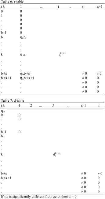
Displaying the elements q and d in tabular form, the structures in Table 7 and 8 can be obtained for each xit: The comments about statistical significance of the r-s algorithm can be apply to thir-s car-se.

Table 6: r-table

j k 1 ... j ... ri ri+1

0 0 1 0 . 0 . 0 . 0

bi-1 0

bi ηi,bi

. . . . . .

k ηi,k

k j 1 j

r− + . .

. . . .

bi+si ηi,bi+si ≠ 0 ≠ 0

bi+si+1 ηi,bi+si+1 ≠ 0 0

. . ≠ 0 0

Table 7: d-table

j k 1 2 ... J ... ri-1 ri

η0ι

0 0

. 0

. . bi-1 0

bi

.

. .

k k j 1

j

d− +

.

. .

bi+si ≠ 0 ≠ 0

bi+si+1 ≠ 0 0

. ≠ 0 0

If ηi0 is significantly different from zero, then bi = 0

Table 8: q-table

j k 1 2 ... j ... ri ri+1 …

0 0

. 0

. .

bi-1 0

bi

. . .

k k j

j

q− .

. .

bi+si ≠ 0 ≠ 0 ≠ 0≠ 0≠ 0

bi+si+1 ≠ 0 0 0 0 0

(7)

221 RESULTS AND DISCUSSION

Empirical results: To illustrate these identification methods, we consider the following simulated model with two inputs[7]:

2 3

3 4

t 1t 2 2t t

1.5L 3L

y (2L 4L )x x N ,

1 L 0.24L t 1,..,100

+

= + + +

− + =

(1-1.3L+0.4L2)Nt = at, at∼N(0,2) (1-1.4L+0.48L2)x1t = ct, ct∼N(0,1) (1-0.7L)x2t = dt, dt∼N(0,2)

In this model at is independent of ct and dt and ct and dt are contemporaneously correlated (with a correlation coefficient of 0.7).

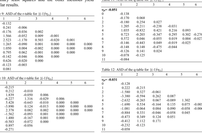
The desired identification pattern is clearly b1 = 3, s1 = 1, r1 = 0 for the first input and b2 = 2, s2 = 1 r2 = 2 for the second one.

Previous results for the corner method and the epsilon algorithm are given in Liu and Hanssens[7] and González-Concepción et al.[8], respectively. They do not differ substantially from those given for the r-s algorithm and the q-d algorithm in Table 9-12 of this study.

The Impulse Response Function (IRF) is now computed using the Cochrane-Orcutt iterative method. Ordinary least squares and the other methods yield similar results.

Table 9: ASD of the r-table for {(-1)j_η 1j}

1 2 3 4 5 6

0 -0.132

1 0.241 -0.006

2 -0.176 -0.036 0.002

3 1.566 -0.052 0.009 -0.001

4 2.523 -1.170 0.503 -0.020 0.001

5 1.265 -0.090 0.001 0.000 0.000 0.000

6 1.050 0.004 -0.002 0.000 0.000 0.000

7 0.795 0.062 -0.001 0.000 0.000

8 -0.142 -0.046 0.006 0.000

9 0.626 -0.020 0.000

10 -0.123 -0.003 11 0.081

1 2 3 4 5 6

0 -0.215

1 0.212 -0.010

2 1.839 -0.050 0.006

3 -6.227 1.316 -0.029 0.006

4 5.428 -0.643 -0.010 0.000 0.000

5 -3.890 0.124 -0.013 0.000 0.000 0.000

6 2.378 0.082 0.002 0.000 0.000 0.000

7 -1.562 -0.093 0.001 0.000 0.000

8 1.480 -0.167 0.001 0.000

9 -0.583 -0.072 0.000

10 0.897 -0.056 11 -0.271

The correct orders for the first input can be adequately identified. For the second input, the possible patterns are (b2,s2,r2) = (2,0,1), (2,0,2), (2,1,1), (2,1,2). In this case, the tables of critical values are not included since the changes in the element values are negligible. Applications:

Economic data: Now we consider some empirical results of these algorithms, using a data set from a leading sales indicator. These data are identified as “series M” in Box and Jenkins[16] and have also been studied by Tsay[14]. The data consist of 150 bivariate observations and were used by these authors to forecast the sales yt using the leading indicator xt.

The TF model found by Box and Jenkins[16] is: 3

t t t

4.82L

y 0.035 x (1 0.54L)a

1 0.72L

∆ = + ∆ + −

−

where, ∆ = −xt (1 0.32L)bt (∆xt = xt – Lxt) is the difference operator and at and bt are white noise processes. The identification pattern is thus b = 3, s = 0 and r = 1, which is clearly confirmed by the corner method given in Box and Jenkins[16]. Tsay[14] carried the investigation further, however, studying the statistical significance of the elements in the corner method. Table 11: ASD of the q-table for {(-1)j_η

1j }

1 2 3 4 5 6

η0= -0.051

0 -0.138

1 -0.170 0.068

2 -0.180 0.254 0.027

3 1.205 -0.211 -0.238 -0.031

4 1.035 -0.832 0.421 0.216 0.093

5 0.723 -0.203 -0.347 0.295 0.302 -0.276

6 0.572 0.046 -0.055 0.019 0.004 -0.027

7 -0.146 -0.443 0.049 -0.019 -0.025

8 -0.148 0.148 -0.475 -0.044

9 -0.126 0.141 0.024

10 -0.078 -0.125

11 -0.084

Table 12: ASD of the q-table for {(-1)j_η 2j}

1 2 3 4 5 6

η0= -0.031

0 -0.128

1 0.222 -0.215

2 -1.580 0.327 -0.061

3 -3.380 -0.594 0.262 0.087

4 -2.632 -0.265 0.067 -0.089 1.302

5 -1.690 0.534 -0.164 0.135 0.075 -0.005

6 -1.081 -0.064 0.084 0.090 -0.058 -0.006

7 -0.884 0.331 -0.046 -0.058 0.045

8 -0.473 0.349 0.124 0.051

9 -0.412 1.112 0.171

10 -0.232 -0.123

(8)

Table 13: ASD of the epsilon table for {(-1)j_η j }

0 1 2 3 4 5 6

0 0.105 1 -0.105 -0.053 2 -0.211 -0.109 0.103 3 10.541 6.419 5.199 4.729 4 -7.800 -0.046 0.025 -0.010 -0.117 5 5.692 0.025 0.002 0.024 -0.082 -0.066 6 -4.360 -0.011 0.025 0.042 -0.032 0.032 0.058 7 3.130 -0.123 -0.083 -0.032 -0.039 0.044 0.051 8 -2.460 -0.017 -0.074 0.033 0.043 0.025 9 1.792 0.189 0.173 0.059 0.051 10 -1.054 0.144 0.162 0.024

11 0.843 -0.086 -0.117

12 -0.843 -0.206

13 0.422

1.28 (3,6,0) (3,0,1)

1.64 (3,6,0) (3,0,1)

1.96 (3,5,0), (3,0,1)

2.33 (3,5,0) (3,0,1)

2.58 (3,4,0) (3,0,1)

2.81 (3,4,0) (3,0,1)

3.09 (3,4,0) (3,0,1)

3.29 (3,3,0) (3,0,1)

3.72 (3,3,0) (3,0,1)

4.26 (3,3,0) (3,0,1)

Table 15: ASD of the r-table

1 2 3 4 5 6

0 -0.208

1 0.122 -0.002

2 0.083 0.000 -0.000

3 -10.998 0.084 -0.001 0.000

4 8.169 -0.410 0.020 0.000 0.000

5 -5.533 -0.176 0.000 0.000 0.000 0.000

6 4.239 -0.177 0.002 0.000 0.000 0.000

7 -2.930 -0.137 0.001 0.000 0.000 8 2.561 -0.152 -0.000 0.000

9 -1.733 0.004 -0.000 10 1.155 0.037

11 -0.976

González-Concepción et al.[8] studied the statistical significance of null entries in the epsilon algorithm table, starting from the results of Berlinet and Francq[3] for ARMA models and adopting the approach of Tsay[14] to compute first-order approximations of the variances in the corner method.

We computed the sequence η and applied the epsilon algorithm to the transformed sequence {(-1)jηj} using SCA software and FORTRAN programming respectively, which yielded the standard deviations table and possible pattern orders in Table 13 and 14.

These results confirm the model proposed by Box and Jenkins[16], which was also obtained by Tsay[14]. Other possible patterns could be given, but they are less parsimonious. Applying the r-s algorithm instead yields the results in Table 15 and 16. Finally, Table 17 and 18 provide results obtained with the q-d algorithm.

1.28 (3,6,0) (3,0,1)

1.64 (3,6,0) (3,0,1)

1.96 (3,5,0), (3,0,1)

2.33 (3,5,0) (3,0,1)

2.58 (3,4,0) (3,0,1)

2.81 (3,4,0) (3,0,1)

3.09 (3,3,0) (3,0,1)

3.29 (3,3,0) (3,0,1)

3.72 (3,3,0) (3,0,1)

4.26 (3,2,0) (3,0,1)

Table 17: ASD of the q-table

1 2 3 4 5 6

η0 = -0.017

0 -0.089

1 0.090 -0.107

2 -0.083 0.082 0.416

3 -5.513 -0.078 -0.048 0.078

4 -3.862 0.351 -0.197 3.282 -1.223

5 -2.820 0.651 -0.191 0.164 0.352 -0.241

6 -2.025 0.187 -0.143 -0.153 0.201 -0.169

7 -1.601 0.594 0.152 -0.130 0.109

8 -1.209 -0.046 0.559 -0.138

9 -0.811 0.016 -0.015

10 -0.621 0.292

11 -0.452

Critical Value Accepted (p,q) models

1.28 (3,4,0) (3,0,1)

1.64 (3,3,0) (3,0,1)

1.96 (3,3,0), (3,0,1)

2.33 (3,2,0) (3,0,1)

2.58 (3,2,0) (3,0,1)

2.81 (3,2,0) (3,0,1)

3.09 (3,1,0) (3,0,1)

3.29 (3,1,0) (3,0,1)

3.72 (3,1,0) (3,0,1)

4.26 (3,0,0) (3,0,1)

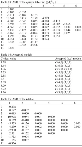
Comparing the results of these four methods confirms that the pattern (3,0,1) is probably the best model.

(9)

223 Next, empirical results provided by the algorithms under investigation are used to illustrate the dynamic relationship between real volatility (an endogenous variable) and the historical and implied volatilities (two exogenous variables). Our sample information (for the Spanish market) consists of 905 observations of the IBEX 35 daily futures price, taken from January 14, 1992, through January 26, 1996.

Due to the limitations of available software packages (SCA, Microfit) in dealing with long series, we decided to use Mathematical to estimate the IRF. We used the Ordinary Least Squares (OLS) approach to calculate the sequences η1 and η2 and standard covariance matrices as input data for algorithms programmed in FORTRAN.

We consider the model for yt (real volatility), x1t (implied volatility) and x2t (historical volatility)

obtained by Gil-Fariña and Lorenzo-Alegría[18] using data taken from November 7, 1994 through September 27, 1995 (200 observations). They estimated the following TF model using SCA software, according to orders identified from the corner method:

t 2 1t 2t

t .0890 .0324L

y x .7082 x

1 1.3626L .9106L

1 .5404L a 1 .2894L

+

∆ = ∆ + ∆

− +

−

where, ∆x1t = −(1 .5654)b ,t ∆x2t =ct and ∆ = 1-L is again the difference operator. The terms at, bt and ct are all white noise processes.

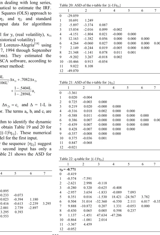
Applying the r-s algorithm to identify the dynamic structure of both inputs, we obtain Table 19 and 20 for the transformed sequence {(-1)jη1j}. These numerical results suggest a (0,1,2) model for the first input.

The results obtained for the sequence {η2j} suggest a (0,0,0) pattern then, the second input has only a contemporaneous effect. Table 21 shows the ASD for the second input.

Table 19: r-table for {(-1)j_η 1j}

1 2 3 4 5 6 7

0 -0.771 1 0.323 0.035

2 -0.185 -0.241 0.263

3 0.486 -0.314 0.349 -0.895 4 -0.136 -0.284 1.976 -0.233 -0.073

5 0.402 -0.336 0.609 0.023 -0.394 1.180 6 0.141 -0.033 1.148 0.416 -0.613 -2.239 3.295 7 0.071 -1.347 1.107 -2.001 2.739 -2.897 8 0.704 -0.817 1.287 3.295 0.393 9 -0.303 0.331 -0.012 0.553 10 -0.344 5.036 -0.578

11 0.297 0.399 12 -1.000

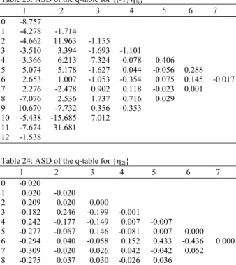
Turning now to the q-d algorithm, we again identify a rational model for the first input. The suggested orders are now (0,1,2), (0,2,2) and (0,3,3), however, which are less parsimonious. The second input is again confirmed to have only a contemporaneous effect on the real volatility. The numerical results of this algorithm are shown in Table 22-24.

1 2 3 4 5 6 7

0 -29.059 1 10.691 1.249

2 -5.897 -3.374 0.087

3 15.034 -2.016 0.099 -0.002 4 -4.151 -1.804 0.021 -0.000 0.000

5 12.163 -1.382 0.056 0.000 0.000 0.000

6 4.264 -0.060 0.027 0.000 0.000 0.000 0.000 7 2.149 -0.244 0.019 -0.005 0.000 0.000

8 21.348 -1.141 0.078 0.011 0.001

9 -9.202 3.267 -0.018 0.002 10 -10.466 0.913 -0.054

11 9.022 8.108 12 -49.070

Table 21: ASD of the r-table for {η2j}

1 2 3 4 5 6 7

0 -3.361

1 0.020 -0.004

2 0.725 -0.003 0.000

3 0.219 0.020 -0.000 0.000

4 -0.316 0.018 0.002 0.000 0.000 5 -0.388 0.011 -0.000 0.000 0.000 0.000 6 0.386 0.007 -0.000 0.000 0.000 0.000 0.000 7 -0.439 0.007 0.000 0.000 0.000 0.000 8 0.428 -0.007 0.000 0.000 0.000 9 -0.357 -0.008 0.000 0.000 10 0.375 -0.036 0.001 11 0.847 -0.068

12 -0.021

Table 22: q-table for {(-1)j_η 1j}

1 2 3 4 5 6 7

η0 = -0.771

0 -0.419

1 -0.574 -7.591

2 -2.621 2.998 -0.118 3 -0.280 0.320 -0.625 -0.408 4 -2.957 3.654 -1.833 -0.089 7.093 5 0.351 0.016 -1.530 18.421 -24.567 3.782 6 0.504 31.014 -32.360 -6.550 2.111 6.017 -0.333 7 9.888 -10.872 0.207 1.331 -0.053 0.000 8 -0.430 0.065 0.005 0.598 0.237

9 1.137 -1.451 47.634 -47.206

(10)

Table 23: ASD of the q-table for {(-1)j_η 1j}

1 2 3 4 5 6 7

0 -8.757 1 -4.278 -1.714

2 -4.662 11.963 -1.155 3 -3.510 3.394 -1.693 -1.101 4 -3.366 6.213 -7.324 -0.078 0.406 5 5.074 5.178 -1.627 0.044 -0.056 0.288 6 2.653 1.007 -1.053 -0.354 0.075 0.145 -0.017 7 2.276 -2.478 0.902 0.118 -0.023 0.001 8 -7.076 2.536 1.737 0.716 0.029

9 10.670 -7.732 0.356 -0.353 10 -5.438 -15.685 7.012

11 -7.674 31.681 12 -1.538

Table 24: ASD of the q-table for {η2j}

1 2 3 4 5 6 7 0 -0.020

1 0.020 -0.020

2 0.209 0.020 0.000 3 -0.182 0.246 -0.199 -0.001 4 0.242 -0.177 -0.149 0.007 -0.007 5 -0.277 -0.067 0.146 -0.081 0.007 0.000 6 -0.294 0.040 -0.058 0.152 0.433 -0.436 0.000 7 -0.309 -0.020 0.026 0.042 -0.042 0.052 8 -0.275 0.037 0.030 -0.026 0.036 9 -0.260 0.042 -0.040 0.037 10 0.341 -0.227 -0.035 11 -0.021 -0.284

12 -0.016

The results obtained confirm the models given in Gil-Fariña and Lorenzo-Alegría[18] and González-Concepción and Gil-Fariña[13].

CONCLUSION

This study highlights the usefulness of several numerical methods (which are all closely related to the PA and OP) in identifying the rational structures associated with data series. We illustrate these methods in the context of causal time series models; that is, ARMA and TF Models.

Special emphasis is placed on the statistical significance of the r-s algorithm and q-d algorithm, in terms of their ASD, as a continuation of several previous contributions in the field of time series analysis.

Empirical findings emphasize the role of this statistical significance in determining the numerical values of the aforementioned algorithms. In general many different possible models may be obtained.

For future research topics, we point out that the correct generalization of these results to VARMA models is not evident. For the corner method, for example, consideration has to be given to the rank of the matrices and not the determinants. The

generalization of the r-s and q-d algorithms to VARMA models has not yet been considered. It would also be of interest to consider the generalization of these numerical algorithms to non-causal contexts, including the estimated future values for the inputs of TF models.

ACKNOWLEDGMENT

This research was partially supported by the National Project I+D+I n° MTM2005-08571 and the Mathematical Research Center of the Canary Islands (CIMAC).

REFERENCES

1. Beguin, J.M., C. Gourieroux and A. Monfort, 1980. Identification of a Mixed Autoregressive-Moving Average Process. In: The Corner Method in Time Series, Anderson, O.D. (Ed.). North-Holland,

Amsterdam, pp: 423-436.

http://www.ams.org/mathscinet-getitem?mr=593345

2. Lii, K., 1985. Transfer function model order and

parameter estimation. J. Time Ser. Anal., 6: 153-169.

DOI: 10.1111/j.1467-9892.1985.tb00406.x

3. Berlinet, A. and C. Francq, 1994. Identification of a Univariate ARMA model. Comput. Stat., 9: 117-133. http://direct.bl.uk/bld/PlaceOrder.do?UIN=023547 806&ETOC=EN&from=searchengine

4. Tiao, G.C. and R.S. Tsay, 1989. Model specification in multivariate time series. J. R. Stat. Soc. Ser. B, 51: 157-213. http://www.jstor.org/stable/2345602

5. Lütkepohl, H. and D.S. Poskitt, 1996. Specification of echelon-form VARMA models. J. Bus. Econ. Stat., 14: 69-79. DOI: 10.2307/1392100

6. Berlinet, A. and C. Francq, 1998. On the identifiability of minimal VARMA representations. Stat. Inference Stochast. Proc., 1: 1-15. DOI: 10.1023/A:1009955223247

7. Liu, L.M. and D.M. Hanssens, 1982. Identification of multiple inputs transfer function models. Commun. Stat. Theor. Math, 11: 297-314. DOI: 10.1080/03610928208828236

8. González-Concepción, C., V. Cano-Fernández and M.C. Gil-Fariña, 1995. The epsilon-algorithm for the identification of a transfer-function model:

Some applications. Numer. Algorithms, 9: 379-395. DOI: 10.1007/BF02141597

(11)

225 10. Brezinski, C., 1980. Padé-Type Approximants and

General Orthogonal Polynomials, Birkhäuser, Basel, ISBN: 3764311002, pp:240-248.

11. González-Concepción, C., M.C. Gil-Fariña and C. Pestano-Gabino, 2006. The statistical significance of some numerical algorithms to identify rational structures in causal time series models. Proceeding of the 5th International Conference on Engineering Computational

Technology, Las Palmas de Gran Canaria, Sept. 12 -15, Civil-Comp Press Stirlingshire, United

Kingdom, Paper 29. http://d.wanfangdata.com.cn/NSTLQK_NSTL_QK

12911201.aspx

12. González-Concepción, C., M.C. Gil-Fariña and C. Pestano, 2007. Some algorithms to identify rational structures in stochastic processes with expectations. J. Math. Stat., 3: 268-276. http://www.scipub.org/scipub/detail_issue.php?V_ No=12&j_id=jms2

13. González-Concepción, C. and M.C. Gil-Fariña, 2003. Padé approximation in economics. Numer. Algorithms, 33: 277-292. DOI: 10.1023/A:1025580409039

14. Tsay, R.S., 1985. Model identification in dynamic regression (distributed lag) models. J. Bus. Econ. Stat., 3: 228-237. DOI: 10.2307/1391593

15. Gray, H.L., G.D. Kelley and D.D. Mac Intire, 1978. A new approach to ARMA modeling. Commun. Stat. Simulat. Comput., 7: 1-77. DOI: 10.1080/03610917808812057

16. Box, G.E.P. and G.M. Jenkins, 1976. Time Series Analysis: Forecasting and Control. Revised Edn., San Francisco, ISBN: 0816211043, pp: 500.

17. Canina, L. and S. Figlewski, 1993. The informational content of implied volatility. Rev. Financ. Stud., 6: 659-681. DOI: 10.1093/rfs/6.3.659