www.atmos-chem-phys.net/14/6369/2014/ doi:10.5194/acp-14-6369-2014
© Author(s) 2014. CC Attribution 3.0 License.
The importance of vertical velocity variability for estimates of the
indirect aerosol effects
R. E. L. West1,*, P. Stier1, A. Jones2, C. E. Johnson2, G. W. Mann3, N. Bellouin2,**, D. G. Partridge1, and Z. Kipling1 1Department of Physics, University of Oxford, Oxford, UK
2Met Office Hadley Centre, Exeter, UK
3National Centre for Atmospheric Science, University of Leeds, UK *now at: Department for Environment, Food & Rural Affairs, London, UK **now at: Department of Meteorology, University of Reading, Reading, UK
Correspondence to:P. Stier ([email protected])
Received: 2 September 2013 – Published in Atmos. Chem. Phys. Discuss.: 17 October 2013 Revised: 13 April 2014 – Accepted: 28 April 2014 – Published: 26 June 2014
Abstract.The activation of aerosols to form cloud droplets is dependent upon vertical velocities whose local variability is not typically resolved at the GCM grid scale. Consequently, it is necessary to represent the subgrid-scale variability of vertical velocity in the calculation of cloud droplet number concentration.
This study uses the UK Chemistry and Aerosols commu-nity model (UKCA) within the Hadley Centre Global En-vironmental Model (HadGEM3), coupled for the first time to an explicit aerosol activation parameterisation, and hence known as UKCA-Activate. We explore the range of uncer-tainty in estimates of the indirect aerosol effects attributable to the choice of parameterisation of the subgrid-scale vari-ability of vertical velocity in HadGEM-UKCA. Results of simulations demonstrate that the use of a characteristic ver-tical velocity cannot replicate results derived with a distribu-tion of vertical velocities, and is to be discouraged in GCMs. This study focuses on the effect of the variance (σw2) of a Gaussian pdf (probability density function) of vertical veloc-ity. Fixed values ofσw (spanning the range measured in situ by nine flight campaigns found in the literature) and a config-uration in whichσwdepends on turbulent kinetic energy are tested. Results from the mid-range fixedσwand TKE-based configurations both compare well with observed vertical ve-locity distributions and cloud droplet number concentrations. The radiative flux perturbation due to the total effects of anthropogenic aerosol is estimated at −1.9 W m−2 with
σw=0.1 m s−1, −2.1 W m−2 with σw derived from TKE,
−2.25 W m−2 with σ
w=0.4 m s−1, and −2.3 W m−2 with
σw=0.7 m s−1. The breadth of this range is 0.4 W m−2, which is comparable to a substantial fraction of the total di-versity of current aerosol forcing estimates. Reducing the un-certainty in the parameterisation ofσwwould therefore be an important step towards reducing the uncertainty in estimates of the indirect aerosol effects.
Detailed examination of regional radiative flux perturba-tions reveals that aerosol microphysics can be responsible for some climate-relevant radiative effects, highlighting the importance of including microphysical aerosol processes in GCMs.
1 Introduction
The indirect effects of anthropogenic aerosols – through their interactions with clouds – are currently one of the most un-certain perturbations to the radiative energy balance at the top of the atmosphere (Forster et al., 2007). A crucial link between aerosol and cloud is that aerosols can act as cloud condensation nuclei (CCN) in a process known as aerosol ac-tivation (Köhler, 1936). This microphysical process must be parameterised if the large-scale effects are to be represented in a general circulation model (GCM), and several parame-terisations have been developed, evaluated and implemented in GCMs in the last decade (see Ghan et al., 2011).
velocity of the rising air. Typically, the large-scale vertical velocities resolved at the GCM grid scale are small, and it is the unresolved subgrid-scale fluctuations which give rise to the updraughts associated with cloud formation. It is there-fore necessary to account for this subgrid-scale variability if aerosol activation is to be represented meaningfully in a GCM.
In local Köhler-theory-based aerosol activation parame-terisations (e.g. Abdul-Razzak et al., 1998; Nenes and Se-infeld, 2003; Ming et al., 2006; Shipway and Abel, 2010), the number of activated aerosols is predicted as a function of aerosol properties (size, number and composition),ai(i=
1...n), vertical velocity,w, temperature,T, and pressure,p, such that it can be expressed asNa(a1, ..., an, T , p, w). The
average number of activated aerosols within a grid box is denoted as Na. Such parameterisations are typically based upon adiabatic parcel model theory and have different levels of complexity.
The problem of representing subgrid-scale vertical veloc-ity has been addressed in current GCMs by two distinct proaches. In the probability density function (pdf)-based ap-proach, it is assumed that the probability density function of vertical velocity within each grid box has an explicit shape,
f (w), assumed continuous (Chuang et al., 1997; Ghan et al., 1997). The grid box parameterisation is thus determined by calculating the expected value of the local parameterisation over each grid box:
Na= R∞
0 Na(a1, ..., an, T , p, w)f (w)dw
R∞
0 f (w)dw
. (1)
Since aerosol activation does not occur in regions of down-draught, integration is only carried out forw >0.
By contrast, in the characteristic approach, it is assumed that the grid-box parameterisation can be obtained by sim-ply substituting a characteristic vertical velocity,w∗, into the local parameterisation:
Na=Na(a1, ..., an, T , p, w∗). (2)
(An obvious motivation for this simplification is the reduc-tion in computareduc-tional expense by eliminating the integrareduc-tion required by the pdf-based approach at every timestep.) The method by which this average number of activated aerosols,
Na(calculated by either method), is then related to the grid-box mean in-cloud droplet number concentration,Nd, is dic-tated by whether the droplet number is treated prognostically or diagnostically by the particular cloud scheme available within the host GCM.
The paper is divided into four sections. Following the in-troduction in Sect. 1, Sect. 2 provides a brief overview of the host GCM and a description of the newly implemented mechanistic aerosol activation scheme within it. Section 2 also contains a description of the model configurations used to assess the model sensitivity toσw, the standard deviation of a Gaussian distribution of vertical velocities. Section 3
contains the results of this experiment, and presents the im-pacts of different vertical velocity configurations on cloud droplet number concentration (CDNC) and liquid water path. The model is evaluated against in situ measurements of CCN, CDNC and vertical velocity statistics in Sect. 3.3. Results of radiative flux perturbation experiments to estimate the radia-tive effects of aerosols in each of the vertical velocity con-figurations are given in Sect. 3.4. These results also highlight some interesting effects due to aerosol microphysics. Finally, conclusions are drawn in Sect. 4. The remainder of this intro-duction provides a review of the characteristic and pdf-based approaches to the representation of vertical velocity variabil-ity, based on the Appendix to Golaz et al. (2011).
1.1 Characteristic vertical velocity
The first attempts to use model-derived vertical velocity in calculations ofNdrelied upon the estimation ofw∗, a single “characteristic” value ofwfor each grid box e.g. Lohmann et al. (1999) usedw∗= ¯w+c√TKE, wherew¯ is the large-scale grid-box mean vertical velocity, TKE the turbulent ki-netic energy and c an empirically derived factor. This ap-proach was adopted by Takemura et al. (2005) and Goto et al. (2008), and adapted by Lohmann (2002) and Ming et al. (2007). An alternative approach, taken by Morrison and Gettelman (2008) and Gettelman et al. (2008), was to derive w∗ directly from the eddy diffusivity, K, and a constant characteristic mixing length, lc=30 m, via w∗= maxKl
c,0.1
m s−1.Wang and Penner (2009) use an amal-gamation of both the Lohmann et al. (1999) and Morrison and Gettelman (2008) formulations. However, with increas-ing computincreas-ing power, this method has been largely super-seded by the pdf-based approach.
Interest in the concept of characteristic updraught has been recently rekindled in the literature (Morales and Nenes, 2010), but Sect. 3.2.4 of this study highlights the limitations of this approach, showing the results of applying the analyt-ical expressions derived by Morales and Nenes (2010) over the full range of aerosol conditions simulated by a GCM. 1.2 Pdf-based approaches to subgrid-scale variability Currently, a prevalent choice of representation of the subgrid variability of vertical velocity is the pdf, and most models that use this approach assume a Gaussian distribution of ver-tical velocities across the grid box, with meanw¯ and standard deviationσw:
f (w)=√ 1
2π σw exp
"
− (w− ¯w)
2
2σ2 w
!#
. (3)
studies, σw became more commonly related to some mea-sure of turbulence within the model. As discussed by Ghan et al. (1997), many processes can produce subgrid-scale vari-ability in vertical velocity, but Ghan et al. (1997) assume that all subgrid-scale variability is due to turbulence;σwwas di-agnosed from the turbulent kinetic energy (if predicted by the host GCM, e.g. Eq. 6) or related to the eddy diffusiv-ity byσw=max
√ 2π K
1z ,0.1
m s−1, where1zis grid-box height. The lower limit of σw=0.1 m s−1 is imposed be-cause turbulence driven by radiative cooling at the cloud top is poorly resolved above the planetary boundary layer in GCMs with coarse vertical resolution>100 m (Ghan et al., 1997). In subsequent studies, this lower limit was raised to
σw=0.2 m s−1 (Ghan et al., 2001a, b; Easter et al., 2004), and later toσw=0.3 m s−1 (Storelvmo et al., 2006). In the most recent modelling study that falls into this category, a much higher minimum value ofσw=0.7 m s−1was used in the reference case and found to occur 98 % of the time (Go-laz et al., 2011); 0.7 m s−1is well above the average recorded
σwacross the flight campaigns through stratiform cloud con-sidered in Sect. 2.4 of the present study and therefore apply-ing such a high, fixed value in 98 % of cases is surprisapply-ing. Hoose et al. (2010) provide a summary of different formula-tions forσwandw∗used in a variety of global models. They compare the behaviour of four parameterisations within the CAM-Oslo global aerosol–climate model (Storelvmo et al., 2006; Hoose et al., 2009) with observations and large eddy simulations from different flight campaigns. This work sug-gests that more widespread evaluation of simulated values of
σw would be useful, and that caution should be exercised in the use of such lower limits onσw.
The functional form off (w)may vary depending on cloud regime, boundary layer type and diurnal cycle (amongst other factors), and the processes governing this shape are far from understood and hence difficult to parameterise. Observations show that a Gaussian distribution may be a reasonable ap-proximation for marine stratocumulus cloud (Peng et al., 2005). However, the subgrid variability of vertical velocity in other cloud regimes may be better approximated by other forms off (w). In situ observations from intensive aircraft campaigns, as well as longer-term statistics from permanent ground-based remote-sensing stations, in different regimes show that variance, skewness and kurtosis of vertical veloc-ity distributions vary not only between different cloud types (Zhu and Zuidema, 2009), but also between clouds of the same type (Moyer and Young, 1991), and even within the vertical profile of a single cloud (Ghate et al., 2010). Hogan et al. (2009) presented ground-based measurements of neg-ative skewness of vertical velocity associated with cloud-driven mixing and showed that the sign of the skewness can vary within the same column below the cloud deck when un-der the influence of both surface-based and cloud-driven tur-bulence. This makes general parameterisation for use at the grid scale in GCMs particularly challenging.
Nevertheless, ongoing developments are underway to im-prove on the basic, initial approximation of a Gaussian pdf. Larson et al. (2002) used a combination of aircraft data and large eddy simulations (LES) to show that a double (bi-nomial) Gaussian pdf provides the best representation of subgrid-scale variability in boundary layer cloud, out of five families of analytical pdfs tested, when compared to ob-served distributions from stratocumulus, cumulus and clear boundary layers measured during two flight campaigns (Al-brecht et al., 1988, 1995). Following on from this, a turbu-lence cloud parameterisation based on the double Gaussian pdf has been developed (Golaz et al., 2002, 2007) and has re-cently been extended to the prediction of cloud droplet num-ber in the single-column version of the GFDL GCM (Guo et al., 2010). This approach has recently been implemented in two separate GCMs (Guo et al., 2013; Bogenschutz et al., 2013).
An alternative approach may be to use a nested modelling framework, in which a LES or cloud-resolving model could be directly activated by GCMs in the most important bound-ary layer cloud-forming regions (Zhu et al., 2010). Currently, this approach is in the early development stages, but with po-tential increases in computational power in the future, it may prove to be useful.
In this study, we use a Gaussian pdf of vertical velocities and focus on exploring the effects of using a range of fixed values ofσw, as well as an experiment in whichσwis derived from the model turbulent kinetic energy. Currently, measure-ments of vertical velocity statistics are so geographically and temporally sparse that even if a more complex functional form off (w) were deployed, its usefulness could only be informed by a very limited set of measurements. It would be difficult to evaluate whether it constituted a global improve-ment compared to observations, other than in the very limited temporal and spatial regime of such observations. For this reason, the added complexity of higher moments off (w)is not yet justifiable in a GCM, and this work will focus on the first and second moments alone, that is, the mean and stan-dard deviation. A more extensive, co-ordinated measurement effort, in conjunction with further LES studies, would be re-quired to make further progress on the parameterisation of subgrid vertical velocity variability for GCMs.
2 Microphysical aerosol–cloud interactions in HadGEM-UKCA
2.1 Modelling framework overview
The modelling framework used for this study is the composition–climate model, HadGEM-UKCA (http://www. ukca.ac.uk), which extends the Hadley Centre Global En-vironmental Model (HadGEM) with an aerosol–chemistry sub-model coupled to the general circulation model radiation scheme. We run HadGEM-UKCA version 7.3 in atmosphere-only configuration, whereby sea-surface temperatures and sea-ice extent are prescribed as seasonally varying fields, with the atmosphere model being a developmental version of the third generation of HadGEM (Hewitt et al., 2011).
All integrations of the model described in this paper utilise this configuration on a staggered Arakawa C-grid (Arakawa and Lamb, 1977) with a resolution of N96 (1.25◦ latitude
×1.875◦ longitude). A staggered Charney–Phillips grid is used in the vertical with 38 levels extending up to 39 km. The dynamical timestep corresponding to this resolution is 30 min.
Coupled within the climate model, UKCA uses compo-nents of HadGEM3 for the large-scale advection, convective transport, and boundary layer mixing of its chemical tracers. Large-scale transport is based on the new dynamical core im-plemented in HadGEM by Davies et al. (2005). Advection is semi-Lagrangian with conservative and monotone treatment of tracers. Convective transport is treated according to the mass-flux scheme of Gregory and Rowntree (1990) and is applicable to moist convection of all types (shallow, deep, and mid-level) in addition to dry convection. For boundary layer mixing, UKCA uses the boundary layer turbulent mix-ing scheme of Lock et al. (2000) which includes a represen-tation of non-local mixing in unstable layers and an explicit entrainment parameterisation.
HadGEM-UKCA is available with either tropospheric chemistry (Telford et al., 2010; O’Connor et al., 2014) or stratospheric chemistry (Morgenstern et al., 2009). A whole-atmosphere chemistry scheme that combines both ap-proaches is also currently in development. Simulations pre-sented in this study use the standard tropospheric chemistry scheme (StdTrop) with aerosol chemistry to couple it to the GLOMAP-mode aerosol microphysics module (Mann et al., 2010), as in the studies by Bellouin et al. (2013) and Kipling et al. (2013). The StdTrop chemistry simulates the Ox, HOx and NOx chemical cycles and the oxidation of CO, ethane and propane with eight emitted species, 102 gas-phase re-actions, 27 photolysis reactions and interactive wet and dry deposition schemes.
The aerosol chemistry extension to StdTrop additionally treats the degradation of sulfur dioxide (SO2), dimethyl sul-fide (DMS) and a monoterpene tracer. In addition, two trac-ers are used to represent species required for the processes of aerosol nucleation and condensation within
GLOMAP-mode: sulfuric acid (H2SO4) produced from the oxidation of SO2with the hydroxyl radical (OH), and a secondary organic species representing the condensable species from monoter-pene oxidation. The oxidation of SO2within clouds is also included, with aqueous sulfate produced via reactions with dissolved hydrogen peroxide (H2O2) and ozone (O3).
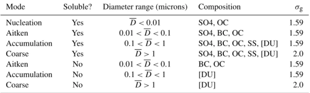
Aerosol modelling in UKCA is accomplished with a modal version of the Global Model of Aerosol Processes (GLOMAP) (Spracklen, 2005; Spracklen et al., 2008), known as GLOMAP-mode (Mann et al., 2010). This is a two-moment pseudo-modal scheme which carries both aerosol number concentration and component mass as prognostic tracers. The aerosol dynamics framework follows that of the M7 model (Vignati et al., 2004). Details of the aerosol modes and the permitted component species within each mode are given in Table 1.
Although dust is a core component resolved within GLOMAP-mode (e.g. Mann et al., 2010), when the scheme is used within HadGEM-UKCA, dust is transported via the existing six-bin scheme (Woodward, 2001). (This aspect of UKCA is still under development, as is the inclusion of am-monium nitrate as an aerosol component.)
Within GLOMAP-mode, aerosol processes are repre-sented following the approach of the original sectional aerosol model, GLOMAP-bin (Spracklen, 2005; Spracklen et al., 2008; Mann et al., 2012). This includes nucleation of sulfuric acid, condensation, coagulation and cloud process-ing. Direct size-resolved emissions of sulfate, black carbon, organic carbon and sea salt particles are included, and sec-ondary aerosol production from sulfur and terpene oxidation is taken into account. The oxidation of mono-terpene by O3, OH and NO3is included explicitly, but the condensable prod-uct yield is fixed at 0.13 %. Hygroscopic growth of all modes and ageing of insoluble modes by condensation or coagula-tion with soluble components are included. Finally, aerosol removal by both dry and wet deposition (sedimentation and scavenging) are also included. Full details of these processes are given by Mann et al. (2010).
2.2 Interactions between aerosols, chemistry and radiation
Table 1.Configuration of the GLOMAP-mode aerosol scheme, with component species: sulfate (SO4), sea salt (SS), black carbon (BC), organic carbon (OC), and dust (DU). Note that dust is not currently available for use in UKCA.Dis the geometric mean diameter andσgthe geometric standard deviation defining each log-normal mode.
Mode Soluble? Diameter range (microns) Composition σg
Nucleation Yes D <0.01 SO4, OC 1.59
Aitken Yes 0.01< D <0.1 SO4, BC, OC 1.59 Accumulation Yes 0.1< D <1 SO4, BC, OC, SS, [DU] 1.59
Coarse Yes D >1 SO4, BC, OC, SS, [DU] 2.0
Aitken No 0.01< D <0.1 BC, OC 1.59
Accumulation No 0.1< D <1 [DU] 1.59
Coarse No D >1 [DU] 2.0
configuration to enable clean forcing experiments and pro-cess studies (e.g. Bellouin et al., 2013).
The refractive index of each aerosol mode varies with the changing internal composition of the mode, and is calculated interactively by volume averaging. Mie look-up tables are then used to obtain the aerosol optical properties (i.e. the specific scattering and absorption coefficients and the asym-metry parameter, which describes the angular dependence of scattering). These allow the direct interactions of aerosol with both longwave and shortwave radiation to be modelled. 2.2.1 Indirect aerosol effects
The focus of this study is on the indirect radiative effects of aerosol, via its interaction with cloud. Aerosol activation is critically dependent on the number, size and composition of aerosols, as well as the local supersaturation of water vapour. The new UKCA activation scheme described here explicitly represents these factors by coupling the dynamically evolv-ing two-moment-modal aerosol scheme GLOMAP-mode to a Köhler-theory-based aerosol activation parameterisation (Abdul-Razzak and Ghan, 2000) to diagnose cloud droplet number concentration.
The indirect aerosol effects themselves are simulated fol-lowing a standard method (e.g. see Jones et al., 2001). HadGEM3 uses the PC2 (prognostic cloud fraction and con-densation) cloud scheme (Wilson et al., 2008), in which cloud droplet number concentration (Nd) is a purely diag-nostic quantity, derived directly from the expected number of aerosols that are available to activate at each time step (Na). Cloud droplet number concentration is used in the calculation of liquid cloud droplet effective radius (re), which allows the cloud albedo effect to be modelled. In the Edwards–Slingo radiation code in HadGEM3, this effective radius is parame-terised following Martin et al. (1994):
re=
3 4π
ρairqc
ρwkNd 1/3
, (4)
whereqcis the cloud liquid water content(kg kg−1)andρair and ρw the densities of air and liquid water. The value of
krepresents the cloud droplet spectral dispersion, and is set to empirically derived values of 0.67 over land and 0.8 over ocean (Martin et al., 1994).
For large-scale precipitation, the rate of increase of rain water by autoconversion of cloud droplets to precipitation,
Rauto,is parameterised as
Rauto=
0.104gEcρ
4 3
air
µρ
1 3
w
q
7 3
c
N
1 3
d
, (5)
whereg is the acceleration due to gravity andµ is the dy-namic viscosity of air.Ecis the collision/collection efficiency of cloud droplets (assumed to be 0.55, Tripoli and Cotton, 1980). Within the scheme, autoconversion occurs when the liquid water content,qc, is above a certain threshold. Once in progress, the process of autoconversion is numerically pre-vented from decreasing the liquid water content below this threshold value.Rautois also dependent on Nd (and hence aerosol), as shown in Eq. (5). Autoconversion is allowed to proceed when the concentration of cloud droplets with radius greater than 20 µm exceeds 1000 m−3, found by assuming a Khrgian–Mazin modified gamma cloud droplet size distribu-tion.
2.3 Reference model configuration
Table 2.Definitions of vertical velocity pdfs in HadGEM-UKCA configurations.
Reference Standard deviation [m s-1]
sigw0.1 σw=0.1 sigw0.4 σw=0.4 sigw0.7 σw=0.7
TKE_0.1 σw=max q
2
3TKE,0.1
In the simulations performed for this study, HadGEM-UKCA was run in a nudged configuration, that is, Newtonian relaxation was used to adjust the dynamical variables of hor-izontal wind and potential temperature in the free-running GCM towards time-varying fields of ERA-Interim data for the year 2008 (Telford et al., 2008, 2013).
2.4 Representation of subgrid-scale vertical velocity variability
Within HadGEM-UKCA, the subgrid variability of vertical velocity is represented using a Gaussian distribution of verti-cal velocities across the grid box,f (w), with mean,w¯, (taken to be the large-scale grid-box mean vertical velocity) and standard deviation,σw.
To assess the effects of the choice ofσw in the Gaussian distribution of vertical velocity, HadGEM-UKCA has been run in four different configurations, outlined in Table 2. In the first three configurations, sigw0.1, sigw0.4 and sigw0.7, fixed values ofσwat 0.1, 0.4 and 0.7 m s−1are applied uni-versally.
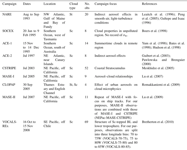
These values have been established from a survey of pub-lished vertical velocity statistics and CDNC, measured in situ by flight campaigns. A range of such campaigns has been se-lected from the literature. A brief summary of the purpose and location of each campaign is given in Table 3. These flight campaigns all focused on marine boundary layer strat-iform cloud. Detailed descriptions of each campaign, the air-craft flown, instrumentation onboard and discussions of the implications of the scientific findings can be found in the ref-erences listed in Table 3.
To establish a representative value of σw, the mean of the values of σw tabulated in each study was taken, and the median was then taken of these mean values, giving 0.4 m s−1. The majority of measured values of σ
w in the set lie within the range 0.1< σw<0.7 m s−1, and these two values—chosen to be equidistant from the median—are then broadly representative upper and lower bounds ofσwwithin stratiform cloud.
In configuration TKE_0.1,σwis estimated from the mod-elled turbulent kinetic energy. Following the method of Ghan et al. (1997), it is assumed that all subgrid-scale variabil-ity in vertical velocvariabil-ity is due to turbulence. HadGEM3 uses the Lock et al. (2000) boundary layer turbulent
mix-ing scheme. This scheme combines non-locally determined eddy-diffusivity profiles for turbulence driven by both sur-face fluxes and cloud-top processes (radiative and evapora-tive cooling), with an explicit parameterisation for the en-trainment rate (derived by Lock, 1998).
The turbulent mixing scheme operates throughout the low-est∼2.5 km of the model troposphere (vertical levels 1 to 11 inclusive), covering the planetary boundary layer and often the lower levels of the free atmosphere. Within these levels, turbulent kinetic energy (TKE) is diagnosed from the mod-elled eddy diffusivity profiles as
TKE=
K
l 2
, (6)
whereKis the eddy diffusivity coefficient andlthe mixing length. Within the planetary boundary layer, l is a combi-nation of boundary layer depth and height above the surface, dependent on the type of boundary layer (Lock and Edwards, 2011; Lock et al., 2000). Above the planetary boundary layer but still within levels 1 to 11, the model contains no physical way of calculating a mixing length in the free atmosphere, so a fixed value ofl=40 m is used to calculate TKE from Eq. (6).
Turbulent kinetic energy per unit mass can be defined as TKE=12 σu2+σv2+σw2. Assuming isotropic turbulence (Ghan et al., 1997; Golaz et al., 2011), this can be approxi-mated by TKE=32σw2, such that within the scope of the tur-bulent mixing scheme,σwcan hence be diagnosed as
σw=max r
2
3TKE, σ min w
!
m s−1. (7)
In levels 12 to 38, above the realm of the turbulent mixing scheme, neitherK norl are calculated, so turbulent kinetic energy is not diagnosed by the model, andσwmust take on a fixed value, chosen here to beσwmin=0.1 m s−1.
3 Results
Table 3.Details of flight campaigns through marine stratiform clouds used for model evaluation.
Campaign Dates Location Cloud
type
No. obs
Campaign focus References
NARE Aug to Sep 1993
NW Atlantic, Gulf of Maine and Bay of Fundy
St 20 Indirect aerosol effects in smooth-air, light-turbulence conditions
Leaitch et al. (1996); Peng et al. (2005); Gultepe and Isaac (1996)
SOCEX 20 Jan to 9 Feb 1995
Southern Ocean, west of Tasmania
Sc 8 Cloud properties in unpolluted region. No record ofσw.
Boers et al. (1998)
ACE-1 15 Nov to 14 Dec 1995
Southern Ocean, south of Australia
Sc 14 Summertime clouds in remote region
Yum et al. (1998); Bates et al. (1998); Hudson et al. (1998)
ACE-2 Jul 1997 NE Atlantic, near Canary Islands
Sc 8 Indirect aerosol effects Guibert et al. (2003);
Pawlowska and Brenguier (2000)
CSTRIPE Jul 2003 NE Pacific, off California
Sc 52 Coastal Stratocumulus Meskhidze et al. (2005)
MASE-I Jul 2005 NE Pacific, off California
Sc 9 Aerosol–cloud relationships Lu et al. (2007)
CLOPAP 30 Sep 2005
Thames Estu-ary and English Channel
St, Sc 4 Effect of urban aerosols on cloud microphysics
Romakkaniemi et al. (2009)
MASE-II Jul 2007 NE Pacific, off California
Sc 11 Repeat of MASE-I with fo-cus on ship tracks. For our purposes, MASE-II observa-tions are combined with those of MASE-I and CSTRIPE (NEPac-MASE-CSTRIPE)
Lu et al. (2009)
VOCALS-REx
16 Oct to 15 Nov 2008
SE Pacific, off Chile
Sc 69 Structure of Sc-topped BL and lower troposphere. For our pur-poses, observations are split into three longitude bins: 70 to 75W (VOCALS-70-75), 75 to 80W (VOCALS-75-80) and 80 to 85W (VOCALS-80-85).
Bretherton et al. (2010)
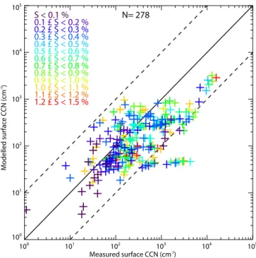
Figure 1 shows a scatter plot of measured versus mod-elled CCN number concentrations, matched by month, loca-tion and supersaturaloca-tion. Measurements taken during obser-vation periods lasting less than a month are plotted against the monthly mean modelled CCN number concentration at the closest value ofS, at the nearest horizontal grid point. For cruise measurements spanning several grid boxes, the grid point closest to the mean of the range of latitude and longi-tude of the cruise is chosen. Measurements from longer ob-servation periods are plotted against the average of the mod-elled CCN values over that period. Errors on CCN measure-ments are assumed to be ±40 % with a minimum absolute uncertainty of 20 cm−3(Spracklen et al., 2011).
In all, 90 % of points are within a factor of ten of the 1:1 line, and the linear Pearson correlation coefficient between the logarithms of the measured and modelled CCN concen-trations isr=0.592. Modelled CCN tend to be biased low compared to the measurements, with a normalised mean bias
of−61.7 %, and this issue is under active investigation. The main deficiency is thought to be due to a low-bias in ma-rine CCN. For example, in Fig. 1 there is a large cluster of points at measured CCN 50–200 cm−3 where the model is consistently low biased by a factor of two compared to the observations. These points are almost entirely for measure-ment locations in the marine boundary layer (MBL), where modelled CCN are known to be biased low in the current model. Future model releases will address this issue.
100
101
102
103
104
105
Measured surface CCN (cm-3) 100
101
102
103
104
105
Modelled surface CCN (cm
-3)
S < 0.1 % 0.1 £ S < 0.2 %
0.2 £ S < 0.3 %
0.3 £ S < 0.4 %
0.4 £ S < 0.5 % 0.5 £ S < 0.6 %
0.6 £ S < 0.7 %
0.7 £ S < 0.8 % 0.8 £ S < 0.9 % 0.9 £ S < 1.0 %
1.0 £ S < 1.1 %
1.1 £ S < 1.2 % 1.2 £ S < 1.5 % 1.5 £ S %
N= 278
Figure 1.CCN measurements from 55 studies, versus co-located
modelled monthly mean surface concentration of CCN at the same supersaturation and location. Points are coloured by supersatura-tion.
3.2 Impacts of different vertical velocity configurations In this section, we examine how differences between each of the configurations of vertical velocity described in Sect. 2.4 affect simulated CDNC and liquid water path (LWP). Fig-ures 2 and 3 illustrate how differences in choice ofσw mani-fests in the annual mean fields of CDNC and LWP. Note that these simulations use present-day aerosols only.
3.2.1 Cloud droplet number concentration
In this paper, annual mean values of CDNC are not weighted by cloud fraction. Instead, a flag is used to identify “cloudy” grid boxes at each time step, and thus to produce in-cloud temporal and spatial averages of CDNC and other cloud properties (where “cloudy” grid boxes are defined as those in which both the cloud liquid water content and liquid cloud fraction exceed zero). While there are shortcomings to this choice, primarily that grid boxes with small and large cloud fractions are weighted equally in the time mean, it was cho-sen for more realistic comparisons with satellite observations and in situ measurements of CDNC, which are not weighted by cloud fraction. CDNC is presented both at liquid cloud-top level (Fig. 2) and at a typical cloud-base level (720 m, Fig. 8c and d) for illustration purposes and for comparison with satellite measurements and in situ observations respec-tively.
Figure 2a shows annual mean CDNC sampled at liquid cloud top in model configuration sigw0.4 (see Table 2).
The choice ofσw can have a significant impact on CDNC, as shown in Fig. 2b, in which the difference in annual mean CDNC at cloud top between model configurations sigw0.7 and sigw0.1 is on average 31.5 cm−3and in excess of 100 cm−3over many continental regions. The magnitude of the global mean relative difference is greatest in regions of high CCN concentration (e.g. over China) where increas-ing the width of the vertical velocity pdf allows activation of much smaller particles. Since the number distribution of aerosols in each mode is log-normal, decreasing the size of the smallest particle that activates can significantly increase the total number activated.
However, the increase in CDNC with increasingσwis only sub-linearly related to the increase inσw, as illustrated in Fig. 2c. An increase ofσw=0.1 toσw=0.4 m s−1leads to a global area-weighted mean increase in CDNC of 21.8 cm−3 but the magnitude of the increase is less than half as large (9.67 cm−3), whenσ
wis increased by the same amount from 0.4 to 0.7 m s−1. Over land, where CCN are saturated, the ef-fect is more pronounced. The non-linearity in this response is due to a levelling-out of the fraction of activation with increasing supersaturation (“fraction of activation” refers to the number of activated aerosols out of the total number of aerosols). Once the fraction of activation is close to unity, further increases inσwcease to have an effect.
3.2.2 Liquid water path
Figure 3a shows annual mean liquid water path in model configuration sigw0.4 (see Table 2). Broadly speaking, in-creasingσwcorresponds to an increase of LWP, particularly over ocean, although the signal is noisy, due to differences in feedbacks between the model runs (shown in the difference between sigw0.1 and sigw0.7 in Fig. 3b).
As shown in Fig. 2b, an increase inσwcan lead to an in-crease inNd, because the higher updraught velocities enable more of the smaller aerosols to activate, due to the increase in maximum supersaturation. Smaller droplets take longer to grow to raindrop size by the collision/coalescence process, thus decreasing the precipitation efficiency of the cloud and increasing the cloud liquid water content.
3.2.3 TKE-derivedσw
In configuration TKE_0.1, the standard deviation of the ver-tical velocity pdf is derived from the local TKE as described in Table 2. In order to see the regions where this dependency has the greatest impact, Fig. 4 shows the difference inσwand
180W 150W 120W 90W 60W 30W 0 30E 60E 90E 120E 150E 180E 90S
60S 30S 0 30N 60N 90N
5 10 20 30 40 60 80 100 120 150 200 250 300 400 600 800 cm-3
-3
(a) CDNC at cloud top: sigw0.4
180W 150W 120W 90W 60W 30W 0 30E 60E 90E 120E 150E 180E 90S
60S 30S 0 30N 60N 90N
-100 -80 -60 -40 -20 0 20 40 60 80 100
cm-3
-3
(b) Difference in CDNC: sigw0.7 − sigw0.1
sigw0.1 sigw0.4 sigw0.7 TKE_0.1
0 10 20 30 40 50 60 70
CDNC in cm
-3
(c) Global mean CDNC
Figure 2. (a) Annual mean cloud droplet number concentration at cloud top in model configuration sigw0.4 (area-weighted mean,
AWM=50.17 cm−3),(b)difference in annual mean CDNC at cloud top between model runs sigw0.7 and sigw0.1 (AWM = 31.50 cm−3) and
(c)global mean CDNC at cloud top for each model configuration. Note non-linear colour bar in(a).
makes significant departures from the reference case (σw= 0.4 m s−1) in both positive and negative directions.
However, most interestingly, other than these rather small differences, comparing Fig. 4a and b demonstrates thatNd from TKE_0.1 is barely greater thanNdobtained in sigw0.4 in any of the other regions where the TKE-derived σw ex-ceeded 0.4 m s−1, such as the persistent stratocumulus region in the southeast Pacific. This indicates that the CDNC in such regions is limited by the low CCN concentration.
3.2.4 Characteristic vertical velocity
HadGEM-UKCA has been used to explore the form of char-acteristic vertical velocity proposed by Morales and Nenes (2010). This study defines the characteristic vertical veloc-ity,w∗, to be the value ofwfor whichNa(w∗)=Na. Essen-tially, an analytical formulation ofw∗is proposed, based on the Twomey (1959) approximation which assumes a power law dependence of the CCN spectrum (i.e.Na=cSk). The characteristic updraught is expressed as w∗=λσw, and an analytical expression is derived to giveλin terms ofk (the steepness of the CCN spectrum).
The values ofλrelevant to a GCM can be calculated by using a pdf of vertical velocities to calculateNdat each grid point within the GCM, but also diagnosing what the char-acteristic updraught would have been at each grid point to give the expected CDNC obtained with the pdf.λcan then be calculated from the known (either prescribed or diagnosed) value ofσw.
Figure 5 shows the annual mean ofλderived in this way from HadGEM-UKCA in configuration sigw0.4. Even in the annual mean,λis highly spatially variable, and takes on val-ues fromλ=0.1 to 0.8 with an area-weighted mean value of 0.5. We note that this range extends considerably lower than the values that Morales and Nenes suggest might be ap-propriate (λ=0.65 derived using the Twomey expression for
Naorλ=0.68 derived from Fountoukis and Nenes, 2005). Given the variable spatial (and temporal, not shown) nature ofλderived from the GCM with a full pdf, it seems inappro-priate to assume that a fixed value ofλwould be suitable for use in a GCM.
180W 150W 120W 90W 60W 30W 0 30E 60E 90E 120E 150E 180E 90S
60S 30S 0 30N 60N 90N
0 10 20 30 40 50 60 70 80 90 100110120130140150160170180190200
gm-2 -2
(a) Liquid water path: sigw0.4
180W 150W 120W 90W 60W 30W 0 30E 60E 90E 120E 150E 180E 90S
60S 30S 0 30N 60N 90N
-10 -8 -6 -4 -2 0 2 4 6 8 10
gm-2
-2
(b) Difference in LWP: sigw0.7 − sigw0.1
sigw0.1 sigw0.4 sigw0.7 TKE_0.1
53.0 53.5 54.0 54.5 55.0 55.5 56.0 56.5 57.0
LWP in gm
-2
(c) Global mean LWP
Figure 3. (a)Annual mean liquid water path in model run sigw0.4 (AWM = 55.63 g m−2),(b)difference in annual mean LWP between
model runs sigw0.7 and sigw0.1 (AWM = 2.28 g m−2), and(c)global mean LWP for each model configuration (note vertical axis shown from 53.0 g m−2upwards).
obtained using 100 000 bins over the range 0< w <10σw
(for 0.1< σw<2.0 m s−1) and thus the computational costs of the pdf-based approach need not be prohibitive. Finally, use of a characteristic updraught would seem to underesti-mate the potential effect of the non-linear relationship be-tweenw∗and CDNC, and hence add unnecessary extra un-certainty to estimates of the indirect aerosol effects.
3.3 Evaluation of CDNC and vertical velocity against in situ measurements
High time-resolution output from each of the configurations of HadGEM-UKCA listed in Table 2, has been co-located in time and space with each of the flight campaigns listed in Table 3 as follows. (Full details of the flight campaigns and aircraft instrumentation may be obtained from the references in Table 3.)
3.3.1 Time
Model output was taken from the whole month of the simula-tion corresponding to the month of the mean date of the mea-surements (albeit with mismatched years), since flight
cam-paigns had a typical duration of three to four weeks. Model diagnostics were output instantaneously every three hours, but only one of these three-hourly time slices was used per day for the appropriate month at each location, since cam-paigns typically made one flight per day (albeit sometimes sampling more than one cloud). For campaigns that pub-lished the time that each flight started, model output for each day of the month was sampled at the time slice closest to the mean flight start time. For campaigns that did not publish times of flights, the time slice closest to 12:00 LT (local time) was sampled, since most flights were made during daylight hours.
3.3.2 Space
The geographic extent of most of the flight campaigns was comparable in area to the horizontal model grid spacing (1.875◦×1.25◦), so model output for each campaign was
180W 150W 120W 90W 60W 30W 0 30E 60E 90E 120E 150E 180E 90S
60S 30S 0 30N 60N 90N
-0.30 -0.24 -0.18 -0.12 -0.06 -0.00 0.06 0.12 0.18 0.24 0.30
ms-1
-1
(a) Difference in
σ
w: TKE_0.1 − sigw0.4
180W 150W 120W 90W 60W 30W 0 30E 60E 90E 120E 150E 180E
90S 60S 30S 0 30N 60N 90N
-100 -80 -60 -40 -20 0 20 40 60 80 100
cm-3
-3
(b) Difference in CDNC: TKE_0.1 − sigw0.4
Figure 4. Annual mean in-cloudσwand CDNC at 720 m. Panels
show differences between model configuration TKE_0.1 with re-spect to sigw0.4 for (a)in-cloudσw (AWM= −0.15 m s−1) and
(b)CDNC (AWM= −12.53 cm−3).
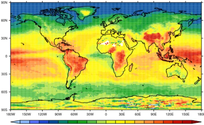
supplementary mission reports. The locations of these flight campaigns is shown in Fig. 6.
Most of the measurements considered in the database were taken at cloud base. In the case of multi-layer clouds, it is as-sumed that aircraft were flown through the lowest layer, since low-level clouds were the focus of most of the campaigns. Therefore, modelled in-cloud properties were sampled at the base of the lowest cloud in a column at that time step, that is, in the lowest “cloudy” grid box, where “cloudy” is defined as any grid box in which both liquid water content and liquid cloud fraction are greater than zero.
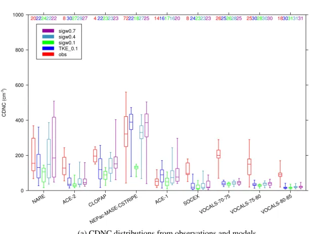
3.3.3 Comparisons between model and observations In Fig. 7a the range, interquartile range and median value of CDNC andσw measured during each flight campaign listed in Table 3 are compared with the same statistics drawn from the co-located model data from each of the configurations listed in Table 2. For each campaign, observations are shown
180W 150W 120W 90W 60W 30W 0 30E 60E 90E 120E 150E 180E
90S 60S 30S 0 30N 60N 90N
0.200.23 0.260.290.32 0.350.380.410.44 0.470.500.530.56 0.590.620.65 0.680.710.74
Figure 5.Annual mean in-cloudλcalculated fromw∗=λσwfrom
model configuration sigw0.4 at hybrid height of 720 m (AWM = 0.51).
NARE ACE-2
CLOPAP CSTRIPE
& MASE
ACE-1 SOCEX VOCALS-REx
180W 150W 120W 90W 60W 30W 0 30E 60E 90E 120E 150E 180E
90S 60S 30S 0 30N 60N 90N
Figure 6.Map of flight campaign locations.
on the left of each group followed by distributions from each model configuration. In Fig. 7b, published observations ofσw are plotted, followed by distributions from TKE_0.1 and appropriate fixed values ofσw for experiments sigw0.1, sigw0.4, and sigw0.7.
Note that both phases of MASE (MASE I & II) and CSTRIPE sampled the persistent stratocumulus cloud deck over the north-east Pacific, off the coast of Monterey, Cali-fornia, in July (albeit of different years), and these measure-ments were aggregated for our purposes and referred to as NEPac-MASE-CSTRIPE.
Model TKE_0.1 shows a good match to the observed me-dian CDNC for NARE. For NARE, the interquartile range (IQR) of CDNC from TKE_0.1 is very similar to the ob-served IQR, although the median and 75th percentile of
NARE ACE-2 CLOPAP
NEPac-MASE-CSTRIPE
ACE-1 SOCEX
VOCALS-70-75 VOCALS-75-80 VOCALS-80-85
0 200 400 600 800 1000
200 400 600 800 1000
CDNC (cm
-3)
2022242222 830272927 422232323 7222182725 1416171620 824232323 2625262825 2530283030 1830313131
obs TKE_0.1 sigw0.1 sigw0.4 sigw0.7
obs TKE_0.1 sigw0.1 sigw0.4 sigw0.7
(a) CDNC distributions from observations and models
Figure 7a.Box-and-whisker plots showing minimum, 25th percentile, median, 75th percentile and maximum values of(a)CDNC and(b)σw,
from flight campaign observations (where reported) in red, and each model configuration (TKE_0.1 in blue, sigw0.1 in green; sigw0.4 in turquoise and sigw0.7 in purple) for marine stratiform flight campaigns. Sample size is given across the top of each figure.
CDNC are slightly overestimated by TKE_0.1 compared to observations for NEPac-MASE-CSTRIPE and ACE-1. For NEPac-MASE-CSTRIPE, it is clear from Fig. 7b that mod-elledσwis too high, since the modelled median far exceeds the median of the observations, and this excess inσw prob-ably leads to some of the excess CDNC in Fig. 7a. That in-creasingσwcan increase CDNC in this region is also evident from the different ranges of CDNC simulated by the three model runs with fixed σw (sigw0.1, sigw0.4 and sigw0.7). However, modelled CCN may also be too high in this region. For ACE-1, it is likely that an excess of modelled CCN is the strongest contributing factor to the excess of CDNC, since the median CDNC from model runs sigw0.4 and sigw0.7 ex-ceeds the median observed CDNC (and is only just less in sigw0.1, for which the prescribed σw is far lower than the observed median ofσw=0.5 m s−1).
CDNC are significantly underestimated by TKE_0.1 for SOCEX, ACE-2, and all three VOCALS cases, compared to observations. One reason for this is that the lowest cloudy model level can occur below the decoupled stratocumu-lus layer, in a region of low TKE. This leads to unrealis-tically low values of σw in some regions, particularly for SOCEX, VOCALS-80-85 and VOCALS-70-75. However, a lack of model CCN is also a significant factor, as discussed in Sect. 3.1. In the VOCALS cases it is clear that low model
CCN dominates the lowσw, since even when the modelled
σwfar exceeds that observed, the number of modelled CDNC is much less than that observed. (For instance, for VOCALS-70–75, the number of CDNC modelled by sigw0.7, is much less than the number observed, even though the median ob-servedσw=0.4 m s−1.) This lack of modelled CCN has been verified with profiles of CCN obtained along the 20◦S
tran-sect of VOCALS-REx (not shown), in which the number concentration of CCN away from coastal sources has a value closer to 200 cm−3 at S=0.4 % (J. Snider, personal com-munication, 2011), compared to low values in the range 20– 50 cm−3 as simulated by the model. The lack of modelled CCN at this location in HadGEM-UKCA could simply be due to a difference between the prescribed aerosol emissions in this region (from the CMIP5 aerosol emissions inventory for the year 2000, Lamarque et al. (2010), compared to what actually happened locally during the VOCALS-REx cam-paign in 2008. However, it is likely that the low CCN bias in the marine boundary layer seen in Fig. 1 plays a significant role in this underestimation, and this issue is under active in-vestigation.
NARE ACE-2 CLOPAP
NEPac-MASE-CSTRIPE
ACE-1 SOCEX
VOCALS-70-75 VOCALS-75-80 VOCALS-80-85 0.0
0.5 1.0 1.5 2.0
σw
(ms
-1)
2022 830 422 6322 1416 024 2625 2530 1830
TKE_0.1 sigw0.1 sigw0.4 sigw0.7
obs TKE_0.1 sigw0.1 sigw0.4 sigw0.7
(b)
σ
wdistributions from observations and models
Figure 7b.Continued.
roles, their importance being dependent on how polluted a region is (Partridge et al., 2012).
3.4 Radiative effects of anthropogenic aerosol
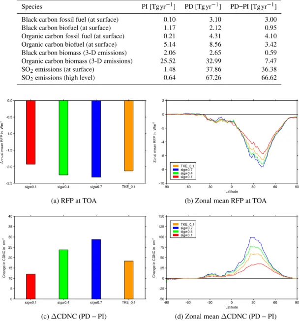
Estimates of the radiative flux perturbation (RFP) due to total anthropogenic aerosol effects, including direct, semi-direct and indirect aerosol effects (cloud albedo and cloud lifetime), and the couplings between them, are derived from the differ-ence in net radiation at the top of the atmosphere between pairs of parallel GCM simulations with present-day (PD) and pre-industrial (PI) aerosol emissions (e.g. Rotstayn and Pen-ner, 2001; Haywood et al., 2009; Lohmann et al., 2010). A summary of the global mean anthropogenic emissions rele-vant to aerosols in the pre-industrial and present-day runs is given in Table 4. The energy imbalance at the top of the atmo-sphere (TOA) ranges from 5.2 to 10.4 W m−2depending on model configuration and aerosol emissions. Since the model was run in atmosphere-only mode for the purposes of this study, some imbalance is inevitable. As with any change to a model that affects radiative fluxes, retuning of the model’s TOA radiation imbalance would be required before employ-ing the scheme for coupled atmosphere–ocean integrations, and such retuning is likely to change the RFP.
The global mean RFP due to anthropogenic aerosol ef-fects from each of the vertical velocity configurations is sum-marised in Table 5 and shown in Fig. 8a.
All four configurations produce a net negative total radia-tive effect due to anthropogenic aerosols, with estimates of the total global mean RFP ranging from −1.9 to a maxi-mum of−2.3 W m−2, depending on choice ofσ
w. It is pos-sible that such a range could have a significant impact on the temperature evolution from PI to PD conditions in a fully coupled model (e.g. Guo et al., 2013). The magnitude of the total radiative effect increases sub-linearly with increasing
σw. Results from an additional pair of simulations with fixed cloud droplet number concentration (not shown) indicate that the RFP due to the direct effect of aerosols alone within HadGEM-UKCA is approximately−0.6 W m−2. Subtracting this value for the direct effect from the four estimates for the total aerosol effects shows the substantial relative variation in magnitude of the modelled indirect aerosol effects due to the choice ofσw.
As discussed in the model evaluation in Sect. 3.2.1, in-creasing σw tends to increase CDNC, since the increased maximum supersaturations provided by the higher updraught velocities possible with a wider pdf enable more of the smaller aerosols to activate.
Table 4.Global emissions from anthropogenic sources for each species considered in this study, for pre-industrial (PI) and present-day (PD) simulations. Emissions for the years 1850 and 2000 are taken from the Coupled Model Intercomparison Project Phase 5 (CMIP5) emissions data set (Lamarque et al., 2010).
Species PI [Tg yr−1] PD [Tg yr−1] PD−PI [Tg yr−1]
Black carbon fossil fuel (at surface) 0.10 3.10 3.00
Black carbon biofuel (at surface) 1.17 2.12 0.95
Organic carbon fossil fuel (at surface) 0.21 4.31 4.10
Organic carbon biofuel (at surface) 5.14 8.56 3.42
Black carbon biomass (3-D emissions) 2.06 2.65 0.59 Organic carbon biomass (3-D emissions) 25.52 32.99 7.47
SO2emissions (at surface) 1.48 37.86 36.38
SO2emissions (high level) 0.64 67.26 66.62
sigw0.1 sigw0.4 sigw0.7 TKE_0.1
-2.5 -2.0 -1.5 -1.0 -0.5 0.0
Annual mean RFP in Wm
-2
(a) RFP at TOA
-90 -60 -30 0 30 60 90
Latitude -10
-8 -6 -4 -2 0 2
Zonal mean RFP in Wm
-2
sigw0.1 sigw0.4 sigw0.7 TKE_0.1
(b) Zonal mean RFP at TOA
sigw0.1 sigw0.4 sigw0.7 TKE_0.1
0 5 10 15 20 25 30 35 40
Change in CDNC in cm
-3
(c)∆CDNC (PD − PI)
-90 -60 -30 0 30 60 90
Latitude -50
-25 0 25 50 75 100 125 150
Change in CDNC in cm
-3
sigw0.1 sigw0.4 sigw0.7 TKE_0.1
(d) Zonal mean∆CDNC (PD − PI)
Figure 8.RFP due to total anthropogenic aerosol effects and change in annual mean CDNC (at 720 m) for model configurations sigw0.1
(red), sigw0.4 (green), sigw0.7 (blue) and TKE_0.1 (orange).(a)and(c)show differences in global mean (PD−PI);(b)and (d)show differences in zonal mean (PD−PI).
surface, for both pre-industrial and present-day conditions for each model configuration. (The aerosol activation scheme was used in all simulations presented in this paper, and there-fore both pre-industrial and present-day CDNC depend on
σwand contribute to the range of indirect aerosol effects.) When considering pairs of simulations with different aerosol emissions, the magnitude of the change in CDNC be-tween the pre-industrial and present-day runs (1CDNC) also tends to increase with increasingσw, as illustrated in Fig. 8d. For instance, the global mean CDNC in the PI run of sigw0.4
is greater than in the PI run of sigw0.1 but, moreover, the higher CCN concentrations in both PD runs leads to much more of an increase in CDNC for the sigw0.4 run than it does for sigw0.1 (i.e. 1CDNC(sigw0.4)> 1CDNC(sigw0.1), shown in Fig. 8d), because the faster updraughts (and hence higher supersaturations) mean that more of the greater num-ber of CCN in the PD run can activate in sigw0.4, and hence the indirect aerosol effects are stronger.
180W 150W 120W 90W 60W 30W 0 30E 60E 90E 120E 150E 180E 90S
60S 30S 0 30N 60N 90N
-10 -8 -6 -4 -2 0 2 4 6 8 10
Wm-2
-2
(a) RFP(sigw0.4)
180W 150W 120W 90W 60W 30W 0 30E 60E 90E 120E 150E 180E 90S
60S 30S 0 30N 60N 90N
-9 -7 -5 -3 -1 1 3 5 7 9
Wm-2 -2
(b) RFP(sigw0.7) − RFP(sigw0.1)
180W 150W 120W 90W 60W 30W 0 30E 60E 90E 120E 150E 180E 90S
60S 30S 0 30N 60N 90N
-9 -7 -5 -3 -1 1 3 5 7 9
Wm-2 -2
(c) RFP(TKE_0.1) − RFP(sigw0.4)
180W 150W 120W 90W 60W 30W 0 30E 60E 90E 120E 150E 180E 90S
60S 30S 0 30N 60N 90N
-11 -9 -7 -5 -3 -1 1 3 5 7 9 11
Wm-2 -2
(d) SWCRE(TKE_0.1) − SWCRE(sigw0.4)
Figure 9. Annual mean radiative flux perturbations due to total (direct and indirect) anthropogenic aerosol effects for(a)model sigw0.4
(AWM= −2.25 W m−2).(b)and(c)show differences in annual mean radiative flux perturbations between(b)sigw0.7−sigw0.1 (AWM= −0.39 W m−2), and (c)TKE_0.1−sigw0.4 (AWM=0.12 W m−2).(d)shows difference in SW CRE for TKE_0.1−sigw0.4 (AWM= 1.18 W m−2).
each of the model configurations. The SW CRE increases with increasingσwfor both PI and PD simulations.
A map of the RFP for sigw0.4 is included in Fig. 9a. Fig-ure 9b and c display difference plots of RFPs between se-lected combinations of model configurations, to highlight the regions where differences manifest themselves in this climat-ically important quantity.
The most striking features of the map of RFP in Fig. 9a are the regions of strong negative RFP, covering much of the ocean in the Northern Hemisphere. The magnitude of this ef-fect increases with increasingσw. Over land regions, the RFP is also predominantly negative, but less so than over ocean, other than in eastern Europe and sweeping out over China into the Pacific outflow region. In these areas the negative effect also intensifies significantly with increasing σw (evi-dent in the difference plot of RFP(sigw0.7)−RFP(sigw0.1) in Fig. 9b).
In the Southern Hemisphere, all model configurations show strong localised negative effects off the coast of Chile in the south-east Pacific ocean and also along the coast of southern Africa. However, other than in these regions, much of the Southern Hemisphere (and tropical) oceans are covered by a weak and noisy positive RFP, which raises some questions. What causes the sign difference be-tween the two hemispheres? In particular, what causes the region of elevated positive RFP in the southeastern Pa-cific? A comparison between the model configurations in-dicates that the intensity of the effect in this region increases with increasingσw (again, evident in the difference plot of RFP(sigw0.7)−RFP(sigw0.1) in Fig. 9b) and is strongest in configuration sigw0.7. This will be addressed further in Sect. 3.5.
Table 5.Global mean RFPs due to total anthropogenic aerosol ef-fects for each of the vertical velocity configurations in HadGEM-UKCA.
Configuration Radiative flux perturbation [W m−2]
sigw0.1 −1.92
sigw0.4 −2.25
sigw0.7 −2.31
TKE_0.1 −2.13
Table 6.Global mean cloud droplet number concentration at 720 m
for each model configuration.
Configuration CDNC (PI) CDNC (PD) Change in CDNC [cm−3] [cm−3] (PD−PI) [cm−3]
sigw0.1 18.41 30.46 12.04
sigw0.4 30.63 54.44 23.79
sigw0.7 36.19 64.99 28.77
TKE_0.1 23.56 41.91 18.35
there are several regions where σw derived from TKE ex-ceeds 0.4 m s−1 (as shown for runs of TKE_0.1 compared to sigw0.4 with present-day aerosol in Fig. 4), the high frequency of occurrence of the minimum value of σwmin in TKE_0.1 brings down the average value ofσw. Both positive and negative features of the map of RFP for TKE_0.1 are re-duced in intensity, compared to sigw0.4, as shown in Fig. 9c. Although allowing σw to depend on TKE produces some regions in which σw>0.4 m s−1, this does not lead to no-ticeable increases in CDNC, compared to that obtained with sigw0.4 (illustrated in Fig. 4a compared to b for present-day aerosol) because, in these regions, CDNC tends to be limited by the number of available CCN rather than updraught. This is particularly true in the marine stratocumulus regions.
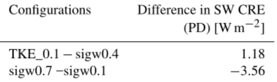
Table 8 shows the difference in present-day SW CRE be-tween pairs of model configurations. The spatial distribu-tion of local features of the CRE between the TKE_0.1 and sigw0.4 is displayed in Fig. 9d and closely mirrors the differ-ence in RFP between those configurations shown in Fig. 9c.
The range of values of RFP generated by the four different vertical velocity configurations provides some quantification of uncertainty in estimates of the RFP due to the choice of pa-rameterisation of vertical velocity. Figure 8b shows the zonal mean RFP due to anthropogenic aerosol effects for each of configurations sigw0.1, sigw0.4, sigw0.7 and TKE_0.1. The overall increasing magnitude of negative effects in the North-ern Hemisphere with increasing σw is more clearly visible here than in the maps shown previously. The behaviour of TKE_0.1 is shown to be closer to sigw0.4 than sigw0.1, as expected from the global mean RFP in Fig. 8a. The near-zero zonal average RFP in the Southern Hemisphere masks signif-icant regional variation, which will be discussed in Sect. 3.5.
Table 7.Global mean shortwave cloud radiative effect (SW CRE)
for each model configuration.
Configuration SW CRE (PI) SW CRE (PD) [W m−2] [W m−2]
sigw0.1 −38.18 −39.10 sigw0.4 −40.56 −41.83 sigw0.7 −41.35 −42.66 TKE_0.1 −39.53 −40.65
Table 8.Difference in global mean SW cloud radiative effect
be-tween pairs of present-day simulations from different model con-figurations.
Configurations Difference in SW CRE (PD) [W m−2]
TKE_0.1−sigw0.4 1.18
sigw0.7 −sigw0.1 −3.56
As described in Sect. 2.4, the choices ofσw for sigw0.1 and sigw0.7 cover the range of the majority of the observed values ofσw recorded in the flight campaigns listed in Ta-ble 3, with very few exceptions. The limited spatial and temporal sampling of this set of observations notwithstand-ing, it is assumed that the range of values in the whole set is broadly representative ofσw in boundary layer strat-iform cloud. Should a fixed value ofσw be required for a GCM, within the boundary layer, it should fall in the range 0.1< σw<0.7 m s−1. Although there may be individual in-stances where σw exceeds these values, to choose a fixed value ofσwoutside of this range to be applied globally would be grossly misrepresentative.
The annual mean RFPs from these two runs therefore pro-vide an upper and lower bound on the effect of the choice of vertical velocity parameterisation on estimates of the RFP in HadGEM-UKCA due to anthropogenic aerosols of−1.9 to−2.3 W m−2. This range is likely to be more sensitive to the choice of bounds at the low end, because the sub-linear dependence of1CDNC (i.e. PD−PI) onσw saturates with increasingσw, and therefore it would be most beneficial to focus further study on forming a tighter constraint on the low end of the range.
As shown in Fig. 7a, both TKE_0.1 and sigw0.4 generate CDNCs that compare reasonably well with those measured in marine stratiform clouds, which provides a degree of confi-dence in the estimates of the RFP. However, the comparisons against the in situ measurements do not provide enough in-formation to quantify whether sigw0.4 or TKE_0.1 is a bet-ter choice of vertical velocity paramebet-terisation to be applied globally. In light of the temporal and spatial variability ofσw shown by the flight campaigns, a parameterisation in which
However, the assumption that this variability can be mean-ingfully approximated by a Gaussian pdf withσw=
q 2 3TKE is still open to further evaluation, and there also remain con-siderable uncertainties in the calculation of TKE itself. It has been proposed that there may be other parameterisations that are more suitable for particular cloud regimes. For ex-ample, Hoose et al. (2010) demonstrated that a liquid wa-ter content (LWC)-based paramewa-terisation can work betwa-ter than a turbulence-based parameterisation for cumulus cloud types. Thus there may be improvements to be made by using cloud regime-dependent parameterisations within GCMs. In the meantime, TKE_0.1 is applied as the default setting for HadGEM-UKCA, with the recommendations that technical issues of high frequency of occurrence of σwmin (due to the lowest cloudy level falling between or just outside the turbu-lent layers, and the lack of properly resolved convective up-draughts), and the choice ofσwminabove the boundary layer, be addressed as a matter of urgency.
3.5 Influence of aerosol microphysics
A slightly surprising feature of the RFP maps shown in Fig. 9 is the positive values visible in the Southern Hemisphere, and in particular the region of elevated positive forcing in the southeastern Pacific. A possible explanation for this is found by considering the microphysical aerosol processes at work in UKCA.
3.5.1 Aerosol mass distributions
The annual mean aerosol burden of each of sulfate, black carbon and organic carbon are shown in Fig. 10.
Results are shown for pairs of runs of model configuration sigw0.4 and illustrate the difference in resulting aerosol bur-den of each component between pre-industrial and present day aerosol emissions.
On average, the sulfate burden has tripled between the PI and PD runs, but the maps show that the increase is far stronger in the Northern Hemisphere (tenfold increases in some regions) than the southern (typical increases of 40 to 80 %). Over land, increases are particularly strong in the in-dustrialised and heavily populated regions of China, India, the Middle East, eastern North America and much of Eura-sia. Sulfate burden has also at least doubled over most of the ocean in the Northern Hemisphere and along the major ship-ping routes through the Southern Hemisphere. This large in-crease in the mass of sulfate in the Northern Hemisphere is a major contributing factor to the strong negative RFP seen in the Northern Hemisphere, due to the increase in CCN, al-though exact details are of course dependent on the size and number distribution of this increased mass. The sharp con-trast between the hemispheres visible in the difference plot of sulfate burden in Fig. 10a is clearly followed through to the contrast between the same regions in the RFP shown in Fig. 9a.
Increases in the black carbon burden due to a combination of fossil fuel combustion and biomass burning has produced a doubling of the global average burden, and substantially greater increases in localised regions. Significant relative in-creases (not shown) have occurred over China and Indone-sia, and over the Amazon, sweeping out across the tropical Pacific. Over eastern North America, the North Atlantic and northern Europe, the black carbon burden has slightly de-creased. The global mean burden of organic carbon has creased 25 % between the PI and PD runs, with strong in-creases in the biomass burning regions and over China. Sim-ilar to black carbon, 40–60 % decreases have occurred over North America, the North Atlantic and northern Europe. The decreases in black carbon and organic carbon over North America arise because of the substantial amount of biomass burning in the 1900 baseline that is used throughout 1850– 2000 in the BC/OC emissions for IPCC AR5 (see Lamarque et al., 2010). The sea salt and dust burdens have not changed between the two simulations (not shown).
3.5.2 Aerosol number distributions
While the difference in total mass of each component is determined by the differences between the prescribed pre-industrial and present-day emissions, the number and size distribution of particles is controlled by UKCA1. The way in which this mass is distributed in terms of particle size and number can significantly affect the CDNC and hence the in-direct aerosol effects.
In the map of RFP shown in Fig. 9, a weak positive ef-fect is visible over the tropical oceans and the oceans of the Southern Hemisphere. This positive region still remains once the direct aerosol effects have been subtracted out from the total effects (not shown). This positive effect is strongest in a region of the southeastern Pacific, and increases in intensity with increasingσw.
The cloud fraction in this region does not change signifi-cantly between the PI and PD runs (not shown). The effect must therefore be brought about by the difference between cloud droplet number concentrations in runs with PI and PD aerosol emissions. Figure 11a shows that the number of cloud droplets is lower in the PD run compared to PI, in the region of positive RFP.
180W 150W 120W 90W 60W 30W 0 30E 60E 90E 120E 150E 180E 90S
60S 30S 0 30N 60N 90N
-80 -70 -60 -50 -40 -30 -20 -10 0 10 20 30 40 50 60 70 80 *10-6 mol m-2
-6 -2
(a) Sulfate (PD − PI)
180W 150W 120W 90W 60W 30W 0 30E 60E 90E 120E 150E 180E 90S
60S 30S 0 30N 60N 90N
-80 -70 -60 -50 -40 -30 -20 -10 0 10 20 30 40 50 60 70 80 *10-6 mol m-2
-6 -2
(b) Black carbon (PD − PI)
180W 150W 120W 90W 60W 30W 0 30E 60E 90E 120E 150E 180E 90S
60S 30S 0 30N 60N 90N
-800 -700 -600 -500 -400 -300 -200 -100 0 100 200 300 400 500 600 700 800 *10-6 mol m-2
-6 -2
(c) Organic carbon (PD − PI)
Figure 10. Change in annual mean aerosol burden by component:(a)sulfate (AWM=23.06×10⁻⁶mol m−2),(b)black carbon (AWM=
8.77×10⁻⁶mol m−2), and(c)organic carbon (AWM=31.26×10⁻⁶mol m−2). All results from pairs of runs of model sigw0.4 run with pre-industrial and present-day aerosol emissions; figures show absolute differences (PD−PI) between pairs of runs.
The response of the RFP in fixedσwruns provides further information. We have shown that CDNC increases with in-creasingσw, because increasingσwcan increaseSmax, which causesamin(the dry radius of the smallest particle which ac-tivates) to be lower, which means that more of the smaller particles can be activated in the higher updraughts. Further, the magnitude of1CDNC between PD and PI – both positive and negative – increases with increasingσw. This could be the result of a number of different effects: a simple increase in the total number of soluble aerosols, while the distribution kept the same shape, or more complex changes to the distri-bution of size, number, mass, or composition between PI and PD runs, as a result of microphysical aerosol interaction.
So, is the number of small, soluble aerosols lower in the PD than PI runs in this region? And if so, why?
Figure 12 shows the change in annual mean number bur-den (column-integrated aerosol number concentration) be-tween pre-industrial and present day simulations for four of
the size modes used in this configuration of UKCA, three sol-uble aerosol modes (nucleation, Aitken, accumulation) and the insoluble Aitken mode. The possible constituent compo-nents of each of these modes is listed in Table 1.
Both soluble nucleation and Aitken modes show a de-crease in the number of particles in the relevant region from PI to PD runs of between 20 and 40 %. It is evident that de-spite increased SO2emissions (not shown, but implied by in-crease in sulfate burden shown previously in Fig. 10), fewer new sulfate particles nucleate in PD conditions, and there are subsequently fewer sulfate particles that can grow into the Aitken mode. The absolute decrease of Aitken mode parti-cles is particularly strong across the tropical Pacific, which corresponds to the region of elevated positive RFP seen in Fig. 9a.