L. E. Zárate
Pontificia Universidade Católica de Minas Gerais Departamento de Ciência da Computação Av. Dom José Gaspar 500, Coração Eucarístico 30535-610 Belo Horizonte, MG. Brazil [email protected]
A Method to Determinate the
Thickness Control Parameters in Cold
Rolling Process through Predictive
Model via Neural Networks
The single stand rolling mill governing equation is a non-linear function on several parameters (input thickness, front and back tensions, yield stress and friction coefficient among others). Any alteration in one of them will cause alterations on the rolling load and, consequently, on the outgoing thickness. This paper presents a method to determinate the appropriate adjustment for thickness control considering three possible control parameters: roll gap, front and back tensions. The method uses a predictive model based in the sensitivity equation of the process, where the sensitivity factors are obtained by differentiating a neural network previously trained. The method considers as the best control action the one that demands the smallest adjustment. One of the capital issues in the controller design for rolling systems is the difficulty to measure the final thickness without time delays. The time delay is a consequence of the location of the outgoing thickness sensor that is always placed to some distance to the front of the roll gap. The proposed control system calculates the necessary adjustment based on a predictive model for the output thickness. This model permits to overcome the time delay that exists in such processes and can eliminate the thickness sensor, usually based on X-ray. Simulation results show the viability of the proposed technique.
Keywords: Steel industry, rolling process, neural networks, controllers
Introduction
The single stand rolling mill governing equation is a non-linear function on several parameters Eq. (1). Any alterations on either of them: input thickness (hi), front (tf) or back (tb) tensions, average
yield stress ( _
y) or friction coefficient (µ) will cause alterations on the rolling load (P) and, consequently, on the outgoing thickness (ho).
) , , , , ,
(P h ,t ,t , y E,R W M
=f
ho i b f µ (1) where: E: Roll radius; R: Roll radius; W: Strip width; and M: Stiffness Rolling Mill modulus (kgf/mm)1
When such alterations in the rolling process occur, three control parameters are mainly used to restore the outgoing thickness and, therefore, ensuring the ∆ho =0 condition: the roll gap, the front and back tensions. The best control parameter will restore the output thickness for its nominal value with the smallest possible adjustment. In this paper, a method to determinate the appropriate adjustment, considering the three control parameters, will be presented. The method uses the sensitivity equation of the process obtained by differentiating a neural network (Zárate 1998). The sensitivity equation corresponds to the predictive model for the cold rolling process, that allows to calculate the output thickness.
To verify the proposed method, a new Automatic Gage Control (AGC) system for output thickness control is proposed. Basically, an AGC system (Wallace, 1964; Hisikawa, 1990) is a feedback control system applied to rolling mills to ensure that output strip thickness will be as constant as possible. To measure the thickness deviations two techniques have been extensively used in the steel industry:
Paper accepted July, 2005. Technical Editor: Anselmo Eduardo Diniz.
a) The first one includes a sensor (X-ray) located after the roll gap, what causes a time delay in the feedback system and produces a significant deterioration in the control performance.
b) The second technique indirectly calculates the output thickness from the measurement of the roll load. This technique presents problems for thin strips, because variations in the strip thickness have little effect on the measured roll load (Zeltkalns and Ricciatti, 1977; Chicharo and Tung, 1990; Zárate, 1998).
The proposed technique in this paper does not follow any of the classical approaches. It uses direct gap measurements to implement the controller. The method uses a neural network and sensitivity factors to obtain the predictive model as proposed in Zárate (1998), Zárate et al (1998 b) and Zárate and Helman (1999). By using a predictive model, it is possible to eliminate the time delay in the feedback loop. Also, since it is based on direct gap measurements, it is possible to achieve the required accuracy for control proposals and elimination of the X-ray sensor.
On the other hand, Artificial Neural Network (ANN) has been receiving a great attention during the last decade, due to the capacity in solving non-linear problems by learning (Hunt, et. al. 1992; Tai et al. (1992), Yamada and Yabuta (1993); Sbarbaro-Hofer, 1993 and Guez et.al. 1998). Nowadays, ANN are receiving great attention in metallurgical processes, as it can be seen in Andersen, et. al. (1992); Smart, (1992); Zárate et. al. (1998a, b); Gunasekera et. al., 1998; Zárate (1998); Zárate and Bittencout (2001); Schlang (2001); Zárate and Bittencout (2002); Kim (2002); Gálvez and Zárate (2003); Yang (2004) and Son (2004).
Nomenclature
_
y = Average yield tensile stress (N/mm2)
g = Gap (mm)
hi = Strip input thickness (mm)
ho = Strip output thickness (mm)
M = Stiffness Rolling Mill modulus (N/mm) P = Rolling load (N/mm)
B
P = Rolling load x Strip width (N) Tq =Rolling Torque (N-mm/mm) R = Roll radius (mm)
tf = Front tension stress (N/mm2)
b
t = Back tension stress (N/mm2) W or B = Strip width (mm.)
E = Young modulus of the strip material
N i
Ui, =0,..., are the net entries and U0=1 is a polarization input
N i
fia(.) =0,..., are the normalization entry functions and
1 (.)
0a =
f N i
Xi, =0,..., are the normalized inputssX0=U0
,..., 0 e ,..., 1
i L j N
Wijh = = is the weight corresponding to the neuron i and entry j
∑
= =
= N
i i h ji h
j W X j L
net
0
,..., 1
product of weights times inputs
1 ) ( with ,..., 0 )
( hj = 0h 0h =
h
j net j L f net
f is the sigmoid function
of the hidden layer. L j
Ij, =0,..., are the corresponding values of the sigmoid function I0=1
,..., 0 e ,..., 1
i M j L
Wijo = = is the weight of the neuron i and
entry j for the hidden layer.
∑ =
=
= L
i i
o ji o
j W I j M
net
0
,..., 1
product of the weights times inputs
for the hidden layer. ,..., 1 )
(net j M
fjo hj = is the value of the sigmoid function for
the exit layer
M j
Yj, =1,..., are the normalized outputs of the net, obtained
from the sigmoid function
M i
fib(.) =1,..., are the an-normalization functions of the
outputs
M i
Zi, =1,..., net outputs values
N k e
emaxk, mink =1,.., higher and lower value of the inputs
M k s
smaxk, mink =1,.., higher and lower value of the outputs
LimiteInf and LimiteSup are the minimum and maximum values of the original data sets respectively.
Greek Symbol
µ = Friction coefficient
Representation of the Rolling Mill Operation through ANN
To represent the cold rolling process operation, Eq. (2), a multi-layer neural network, with six entries (N=6), two exits (M=2) and one hidden layer with 13 neurons (2N+1, Kovács 1996) was used. In expression (2), the neurons have as activation function (f) the non-linear sigmod function, chosen in this work as the axon transfer
function being the most consistent with the biophysics of the biological neuron.
) , ( )
, , , , ,
( o B
ANN f
b
i g t t y h P
h µ → (2)
with y: average yield stress; PB rolling load.
Generally, the largest care to get a trained neural network lies on collecting and processing neural network input data. The pre-processing operation consists in the data normalization in such a way that the inputs and outputs values will be within the range of 0 to 1.
The following procedure was adopted to normalize the input data before using it in the ANN structure:
a) In order to improve convergence of the ANN training process, the normalization interval [0, 1] was reduced to [0.2, 0.8], because in the sigmod function the values [0, 1] aren’t reached: f→ 0 for net→ -∞and f→ 1 for net→ +∞.. b) The data was normalized through the following formula:
) - L n) / (L (Lo - Lmí Ln
(Lo) fa
min max =
= (3a)
fb(Ln) Lo Ln * L ( - Ln) * Lmín
1
max +
=
= (3b)
where Ln is the normalized value, Lo is the value to normalize, Lmin and Lmax are minimum and maximum variable values, respectively.
c) Lmin and Lmax were computed as follows:
Lmín = (4 x LimiteInf. - LimiteSup) / 3 (4a)
Lmáx = (LimiteInf. – 0.8 x Lmín) / 0.2 (4b)
The Eqs. (4a) and (4b) are obtained substituting in the Eq. (3a) Ln = 0.2 and Lo = LimiteInf; and Ln = 0.8 and Lo = LimiteSup. Where LimiteInf and LimiteSup are the minimum and maximum values of the original data sets respectively.
Obtaining the Sensitivity Factors
The expression to calculate sensitivity factors was proposed in Zárate (1998). In this work, an ANN multi-layer with a hidden layer is used. The ANN has N: entries, M: exits and L: neurons in the hidden layer. The differentiation of the neural network is generic and it only depends on N, M, L and on the weights of the hidden and exit layers, obtained during the training process.
− −
−
− −
−
− −
−
= ∂ ∂
N emin N emax
h LN W Q
2 emin 2 emax
h 2 L W Q
1 emin 1 emax
h 1 L W Q
N emin N emax
h N 2 W Q
2 emin 2 emax
h 22 W Q
1 emin 1 emax
h 21 W Q
N emin N emax
h N 1 W Q
2 emin 2 emax
h 12 W Q
1 emin 1 emax
h 11 W Q
W R W
R W R
W R W
R W R
W R W
R W R
i U
k Z
L L
L
2 2
2
1 1
1
o ML M o
2 M M o
1 M M
o L 2 2 o
22 2 o 21 2
o L 1 1 o
12 1 o 11 1
(5)
L k N i i X h ki W N i i X h ki W
Qk 1,...,
2 ) 0 ) ( exp 1 ( 0 ) ( exp = ∑ = − + ∑ = − = M k V V
Rk 1,..,
2 ) k exp 1 ( k exp ) k smin k smax ( − = + − − = M ,..., 1 para ) ) ( ( N 0 L 0 = =
∑
∑
= = k U f W f W V i i a i h ji h j j o kj kNote that Eq. (5) is valid for little variations in the process parameters and provides the linearization of the process for an operation point (Ui) (Zárate et. al. 1998c).
Determination of the Adjustment in the Control Parameters
The steps to determine the adjustments corresponding to the control of the rolling process are described as below:
I. The nominal inputs and outputs are contained in the vectors: ) , , , , , ( * * * * * * * y t t g h
X = i µ b f and ( , )
* * *
P h
Y = o respectively. II. Through Eq. (5), it is possible to calculate the sensitivity
factors for the selected nominal point. After calculating the factors, is possible to obtain the linear equation of the process, Eq. (6), neighboring the nominal operation point:
y h y t h t t h t h g h g h h h h o f o f b o b o o i o i o ∂ ∂ + ∂ ∂ + ∂ ∂ + ∂ ∂ + ∂ ∂ + ∂ ∂ = ∆ ∆ ∆ µ µ ∆ ∆ ∆
∆ (6)
where: ∆X=X *-X
If variation takes place either in one or all the operational parameters hi,g,µ,tb,tf,y, a variation will occur in the hovalue. There is a factor K such that ∆ho=0. Eq. (7):
K y h y t h t t h t h g h g h h h o f o f b o b o o i o i + ∂ ∂ + ∂ ∂ + ∂ ∂ + ∂ ∂ + ∂ ∂ + ∂ ∂ = ∆ ∆ ∆ µ µ ∆ ∆ ∆ 0 (7)
Equating Eq. (6) and Eq. (7), it is obtained:
f
h
K=−∆ (8)
The value of K depends on the selected control parameter: roll gap, front or back tensions and may be defined as:
f o f b o b o t h t K t h t K g h g K ∂ ∂ = ∂ ∂ = ∂ ∂
=∆ or ∆ or ∆ (9)
If control action by means of the roll gap is considered, the equations to calculate the K value are:
g h h g g g h h g h g h g K o o o o o o ∂ ∂ + = ∂ ∂ − = − = ∂ ∂ =∆ ∆ ∆ ∆ * ∆ (10)
Similarly, choosing the front and back tensions:
b o o b b t h h t t ∂ ∂ + = * ∆ (11) f o o f f t h h t t ∂ ∂ + = * ∆ (12)
Observe that expressions (10), (11) and (12) don't depend on the measurement of the rolling load, although it is necessary to know the variation in the exit thickness, which will be obtained indirectly by the predictive model.
Kernel of the Algorithm to Obtain the Control Parameters
In the previous section three possible control parameters were calculated to restore the variations in the output thickness. A strategy to select the appropriate adjustment can be to choose the parameter with the smallest adjustment. The kernel of the proposed algorithm is shown as follows:
on front teni on action control on back tensi on action control gap on action control : * * * f o o f f r o o b b o o t h h t t t h h t t g h h g g calculate Begin ∂ ∂ + = ∂ ∂ + = ∂ ∂ + = ∆ ∆ ∆ ion front tens the of adjustment / 100 * | | Var_ on back tensi the of adjustment / 100 * | | Var_ gap the of adjustment / 100 * | | Var_ : * * * * * * f f f f b b b b t t t t t t t t g g g g calculate − = − = − = . ) action control ( ) action control ( * 85 . 0 * 85 . 0 Var_ Var_ ) action control ( ) action control ( * 85 . 0 * 85 . 0 Var_ Var_ ) action control ( ) action control ( 001 . 0 001 . 0 | | Var_ Var_ e Var_ Var_ * End t Then P If t Then P If S t Then S t If Then t t If else t Then P If t Then P If S t Then S t If Then t t If else g Then P If g Then P If g Then g g If Then t g t g If f f o f o f r f b b i b i b f b f b ↓ ↓ ↑ ↑ = > < ↓ ↓ ↑ ↑ = > <= ↑ ↓ ↓ ↑ = < − < <
the value of the sensitivity of the instrument (by example, 0.001). For back and front tensions the saturation is established in 85% of the yield stress in plane-strain deformation, in the entry (Si) and in the exit (So) respectively.
Predictive Model for Output Thickness
There are several theoretical models to calculate rolling load and rolling torque. The mathematical modeling of the rolling process involves several parameters that may lead to non-linear equations of difficult analytical solution. Such is the case of Alexander's model (Alexander 1972), considered one of the most complete in the rolling theory. This model requires significant computational effort, which prevents its application in on-line control and supervision systems. On the other hand, the theoretical models allow to calculate the rolling load, where the output thickness (ho) is an input parameter of the model. In Zárate (1998). a new representation (predictive model) to determinate the output thickness (Eq. 13), based on sensitivity factors, was presented.
} y y P + P + t t
P + t t P + h h P g+ W M {
h P W M
W =
h f
f b b i i
o
o ∆
∂ ∂ µ ∆ µ ∂ ∂ ∆ ∂ ∂ ∆ ∂ ∂ ∆ ∂ ∂ ∆ ∂
∂ ∆
−
(13)
Those factors are obtained through the differentiation of a neural network previously trained. For this purpose the considered neural network is represented by expression (14):
) , (
)
,
,
,
,
,
(
h
ih
oµ
t
bt
fy
→
ANN
PTq (14)The neural network (Eq. 14) was trained with data of the rolling process during the deformation of the material. The new representation (Eq. 13) possesses predictive characteristics, eliminating time delay and the X-ray sensor of the rolling mill system.
The predictive model can be expressed as:
[ ][ ]
o oo DS u h h
h = ∆ = *−
∆ (15)
or
[ ][ ]
S u D h ho= o− ∆* (16)
where
− =
o h
P W M
W D
δ
δ (17)
with
[ ]
=
y P P t
P t P h P W M S
f r
i δ
δ δµ δ δ δ δ δ δ
δ (18)
and
−
=
=
y t t h
g
y t t h g
y t t h g
u
f r i
f r i
f r i
µ µ ∆
µ ∆ ∆ ∆ ∆ ∆
∆
* * * * * *
(19)
Usually the entries of
[ ]
S are calculated from equations that demand a difficult analytical solution from complex models, such as Alexander’s model. In this work,[ ]
S is obtained through the differentiation of a neural network, using Eq. (5).Control System Proposed
The controllers’ classic development requests the knowledge of the dynamics of the plant besides a linear model for a specific operation point. In rolling systems there are time delays that difficult the development of control systems and that normally present a low performance (Zárate 1998). In addition to this, a characteristic of those systems is the existence of significant time delays of the order of 30 s. This can happen for low rolling speeds, that normally occur in the first stand of a tandem mill.
This work introduces a new control structure, that uses the predictive model, Eq. (16), to estimate the output thickness and the measurement of the gap, Eq. (10). Usually, an AGC measures the rolling load to determinate, through Eq. (20), the necessary adjustment for the gap and to assure the condition ∆ho=0.
M P.B h
g= o
∆ ∆
∆ − (20)
To calculate the adjustment of the gap, the proposed controller structure uses the sensitivity factor ∂ho ∂g in Eq. (10). Observe that ∆ho =ho*−ho uses the predicted value of the output thickness
p o
o h
h = .
Figure 2 shows the controller's structure proposed. Note that the predictive model is being implemented as a virtual sensor whose exit is the output thickness hop.
The Controller PD was projected to adjust the gap calculated by means of the method of the sensitivity, Eq. (10). The controller PI was introduced to eliminate possible errors in the predictive model and to guarantee the condition: h*s−hsp =0.
PD
PI
Predictive Model
(ho) Equation (16)
Rolling Mill Parameters
+
-+
+
+
-1
−
∂ ∂
g ho
*
o
h
*
g
S s 1.08
08 . 1 2+
p o
h
g
Application and Results
As an example of the possibilities of the method, a numerical application to a rolling process will be presented. The operation point was chosen as: h =i 5.0 mm; h = o 3.6 mm; g=1.846 mm.; µ
=0.12; t =f 89.22 N/mm2; tb=4.325N/mm2;
_
y=460.106 N/mm2; B = 500 mm; E = 200054.64 N/mm2; R=292.1 mm; M=4903,300
N/mmand P=875310 N/mm. With: Si =250.556 N/mm2 and
=
o
S
534.900 2N/mm .
To obtain the data sets for training of the neural networks, Eq. (2) and Eq. (14), the parameters were varied as shown in Table 1:
Table 1. Variation of the operational parameters.
i
h ho µ tf tb y
± 8% ± 3% ± 20% ± 30% ± 30% ± 10%
Three different values were chosen for each parameter, resulting in 729 training sets. The rolling load was obtained through Alexander's model and the roll gap by the elastic equations of the rolling mill, Eq. (21).
M PB h
g= o− (21)
For the neural network represented by Eq. (2) (to calculate the control parameters) the final weights for the hidden and output layers with its polarization weights are:
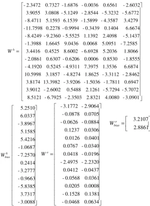
= 4.2330 4.0985 1.5484 11.5151 4.8319 2.9411 4.2602 0.7387 0.0733 1.6808 11.9576 1.4947 1.8826 4.0553 8.1868 5.9967 2.3521 8.3913 2.1458 0.4850 0.0399 0.0338 10.6099 1.2378 1.5593 2.2323 0.1518 7.6049 8.2071 0.8914 8.9722 0.6086 3.4559 6.5208 3.2388 4.8199 -0.9006 7.0447 0.5558 7.4542 3.4810 6.1621 -5.5016 0.9096 9.7730 0.7990 3.9726 8.9832 4.7363 0.5938 0.0343 3.4006 5.2707 3.3504 0.8293 3.3595 0.2737 5.5920 8.3214 0.2767 -3.3125 0.6941 0.2171 1.2562 1.7129 11.4365 -6.0229 0.7813 0.0734 2.4238 9.2425 1.5239 -1.3078 1.8475 0.2642 1.7278 9.4161 6.2010 h W = 2.5081 8.7774 0.4583 8.8376 7.1306 4.5520 5.3887 15.1094 10.4911 10.9804 2.5654 8.9265 11.4784 h bias W = 0.0746 0.1814 2.4463 3.9372 0.0106 0.0276 1.0470 6.4508 0.0074 1.1542 0.0480 0.1378 0.1406 0.1479 0.0045 0.0021 0.9087 4.2976 0.2163 0.2976 0.1960 0.9245 2.1593 1.7551 0.4083 0.5503 o W 1.4106 6.4599 o bias W
The weights were obtained after 330,000 iterations with an average quadratic error of 0.040 (Pentium IV 3.0 GHz).
For the neural network represented by Eq. (14) (to determine the predictive model) the final weights for the hidden and output layers with its polarization weights are:
= 3.0901 4.0080 2.8321 2.3503 6.7925 8.5121 5.7072 5.7294 2.1261 0.5488 2.6002 3.9012 0.6947 1.7811 1.5036 3.9206 13.3982 3.8174 2.8462 3.3112 1.8625 4.8274 3.1857 10.5998 6.6874 1.3536 7.3975 4.9311 0.5245 4.1920 -1.8555 0.8530 0.0006 0.6206 0.6307 2.0861 -1.8066 5.2036 6.6928 8.6002 0.4525 3.4416 7.2585 5.0951 0.0068 9.0436 1.6645 1.3988 -5.1437 2.4098 1.1392 5.5525 9.2360 8.4249 -6.6674 0.1404 0.3439 0.9994 0.2278 11.7598 -3.4279 4.3587 1.5899 6.1539 5.1593 8.4711 -5.6772 5.3232 2.8544 5.1249 3.0808 3.9055 2.6032 0.6561 0.0036 1.6876 0.7327 2.3472 h W 3.0088 3.7317 5.8385 0.9663 3.2777 0.2414 7.2570 1.0687 5.4216 5.1585 3.8967 6.0337 5.2510 h bias W = 0.0634 0.0468 0.1381 0.1528 0.0008 0.0205 0.0361 0.0568 0.0437 0.0412 2.2320 2.4975 0.0196 0.0418 0.0340 0.0767 0.0401 0.0126 0.0306 0.1237 0.0884 0.0626 0.0705 0.0878 2.9064 3.1772 Wo = 2.8861 3.2107 o bias W
The weights were obtained after 540,000 iterations with an average quadratic error of 0.033 (Pentium IV 3.0 GHz).
The events sequence to determine the control operation adjustments are described as follows:
1) Define the nominal inputs: [hi*,g*,µ*,tb*,t*f,y]= [5.00; 1.846; 0.12; 4.324; 89.22; 460.106] and provide the nominal outputs: [ho*,P*]=[3.6; 8583.81];
2) Calculate through Eq. (5) the sensitivity factors for the selected nominal point: [
y h t h t h h g h h h o f o b o o o i o ∂ ∂ ∂ ∂ ∂ ∂ ∂ ∂ ∂ ∂ ∂ ∂ , , , , ,
µ ] = [0.3566;
0.6436; 4.7345; -0.0163; -0.011; 0.0327];
3) Considering, for example disturbances of -2% in the input thickness, in the friction coefficient and in the back tension, define the current entries as: [hi,g,µ,tb,tf,y]= [4.9; 1.846; 0.118; 1.157; 89.22; 460.918];
4) Use an ANN, Eq. (2) previously trained to determine the current outputs: [hs,PB]= [3.552; 8389.81];
5) Determine the three control parameters using Eqs. (10), (11) and (12): [g ,tb tf ] = [1.920; -4.94; 46.42]. That corresponds to corrections of: +3.8%, -639.9% and -54% respectively.
6) Apply proposed algorithm to select the control parameter. The smallest correction indicates the best control action. Notice that the calculated value for tb is negative and this should be saturated
in tb =0. Thus the adjustment for the output thickness should be made through gap.
value of the output thickness was 3.584 mm with error of 0.44%. The smallest error confirms the action on the gap to restore the deviations in the output thickness.
Table 2 shows the sensitivity factors for the nominal operation point obtained by differentiation of the neural network, Eq. (14).
Table 2. Sensitivity Factors (for the Predictive Model).
i h P
δ δ
o h
P
δ δ
δµ δP
b t
P
δ δ
f t
P
δ δ
y P
δ δ
498.66 -631.16 7909.25 -86.56 -5.83 56.75
The sensitivity factor for the adjustment of the gap is obtained in step 2:
g ho
δ
δ =0.6436. The transfer function of the plant considered
in this work is given for:
) 08 . 1 (
08 . 1 ) (
+ =
s s s
G (22)
The controllers’ parameters PD and PI were adjusted by simulation and they were chosen as: KP= 5 and KD= 1.5 for the PD controller and as: KP= 3 and KI = 1.0 for the PI controller.
To analyze the proposed controller, two simulations were accomplished applying disturbance on the rolling parameters (Table 3).
Table 3. Disturbances in parameters.
Parameter t (star) s. t (final) s. Sequence 1 (%)
Sequence 2 (%) i
h 15 30 + 3.0 + 8.0
b
t 45 60 + 10.0 + 30.0
f
t 75 90 +10.0 + 30.0
µ 105 120 + 5.0 + 20.0
y 135 150 + 3.0 + 10.0
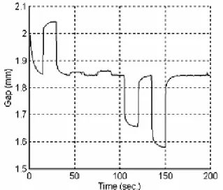
Figure 2 shows the response of the output thickness for the sequence 1. In this case, the controller has an error below 1.4% and the stationary-state was reached in less than 4 s.
Figure 2. Output thickness response for sequence 1.
Notice that the alterations in the back and front tensions are not relevant. For sequence 1, the significant variations are due to disturbances in the average yield stress, in the input thickness and in the friction coefficient. Figure 3 shows the behavior of the gap for the same simulation.
Figure 3. Gap responses for sequence 1.
The last simulation was to verify the proposed controller's robustness. Figure 5 shows the response of the output thickness for sequence 2. This sequence considers typical values of maximum deviations in the rolling processes (Bryant et. al. 1973). Observe that the output thickness of the predictive model uses sensitivity factors obtained for small disturbances in the operation point. In this case, the controller maintained the error in the output thickness below 4.1%, and the response reached the stationary state in 12 s. The Figure 6 shows the response of the gap for this situation.
Figure 5. Gap responses for sequence 2.
Conclusion
In this paper, it was presented a method to determinate the appropriate adjustment for thickness control, considering three possible control parameters: gap, front tension and back tension. This method, a new technique AGC, uses the sensitivity factors to choose the best control parameter.
The proposed control structure uses a predictive model for the output thickness based on neural networks and sensitivity factors. The structure allows to eliminate the time delay presented in the dynamics of the system and to eliminate the thickness sensor, usually X-ray. This control system implements a virtual sensor for output thickness, allowing to estimate "on-line" outgoing thickness. The analysis and simulation results show that the proposed structure has results that are acceptable for rolling processes. The predictive model uses sensitivity factors calculated in the neighborhood of an operation point and it was observed that the control system had a satisfactory behavior for great deviations in the nominal operation point.
References
Alexander, J.M., 1972, “On the theory of Rolling”. Proc. R. Soc. Lond. A. 326, pp. 535-563.
Andersen, K., Cook, G.E. and Barnett, R.J., 1992, “Gas Tungsten Arc Welding Process Control Using Artificial Neural Networks”, International Trends in Welding, Science and Technology, ASM, pp. 877-1030.
Bryant, G.F., Edwards, W.J. and McClure, C.H., 1973, “Automation of Tandem mills”, London: The Iron and Steel Institute. Cap. 1,pp.1-29.
Chicharo, J.F. and Tung, S., 1990, “A roll eccentricity sensor for steel-strip rolling mills”, IEEE Trans. on Industri Applications, Vol. 26, N° 6, Nov/Dez, pp. 1063-1069.
Guez, A., Eilbert, J. L. and Kam, M., 1988, “Neural Network Architecture for Control”, IEEE Control Systems Magazine, vol. 8, pp. 22-25.
Gunasekera, J.S., Zhengjie Jia, Malas J.C., Rabelo, L.1998, “Development of a neural network model for a cold rolling process”, Engineering Applications of Artificial Intelligence, Vol. 11, pp. 597-603.
Hishikawa, S., Maeda, H., Nagakura, H, Hattori, S., Nakajima, M. and Katayama, Y., 1990, “New Control Techniques for Cold Rolling Mills – Applications to Aluminum Rolling”, Vol. 39, N° 4, pp. 221-230.
Hunt, K.J., Sbarbaro, D., Zbikowski, R., and Gawthrop, P.J., 1992, “Neural Networks for Control, A Survey”, Automatica, vol. 23, No. 6, pp. 1083-1112.
Kim, D.H., Lee, Y. and Kim B.M., 2002, “Applications of ANN for the dimensional accuracy of workpiece in hot rod rolling process”, Journal of Materials Processing Technology”, Vol. 130-131, pp. 214-218.
Kovács. Z.L. 1996, “Redes Neurais Artificiais”, Edição Acadêmica São Paulo, Cap 5, pp.75-76. São Paulo. Brasil.
Sbarbaro-Hofer, D., Neumerkel, D. and Hunt, K., 1993, “Neural Control of a Steel Rolling Mill”, IEEE Control Systems, June, pp. 69-75.
Shlang, M. Lang, B. Poppe, T., Runkler T., Weinzier K., 2001, “Current and Future development in neural computation in steel processing”, Control Engineering Practice, Vol. 9, pp. 975-986.
Smartt, H.B., 1992, “Intelligent Sensing and Control of Arc Welding”, International Trends in Welding, Science and Technology, ASM, pp. 843-851.
Son, J.S., Lee, D.M., Kim, I.S. and Choi, S.K. 2004, “A study on genetic algorithm to select architecture of a optimal neural network in the hot rolling process”, Journal of Materials Processing Technology”, Vol. 153-154, pp. 643-648.
Tai, H. M., Wangi, J. and Ashenayi, K., 1992, “A Neural Network-Based Control System”, IEEE Transactions on Industrial Electronics, vol. 39, no. 6, pp. 504-510.
Wallace, J.W., 1964, “Fundamentals of strip mill Automatic Gage Control Systems”, Iron and Steel Engineer, September, pp 193-202.
Yamada, T., and Yabuta, T., 1993, “Dynamic System Identification Using Neural Networks”, IEEE Transactions on Systems, Management, and Cybernetics, vol. 23, No.1.
Yang, Y.Y., Linkens, D. and Talamantes-Silva, 2004, “Roll load prediction – data collection, analysis and neural network modelling”, Journal of Materials Processing Technology”, Vol. 152, pp. 304-315.
Zárate, L.E., 1998, Tese de Doutorado, "Um Método para Análise da Laminação Tandem a Frio", Universidade Federal de Minas Gerais, Escola de Engenharia Metalurgica e de Minas, Belo Horizonte, MG, Brasil.
Zárate, L.E., and H. Helman, J.M. Gálvez 1998a, Um Modelo para Processos Baseados em Fatores de Sensibilidade, Utilizando Redes Neurais. XII CBA, Vol. I, pp.23-28, September 14-18, Uberlândia, MG, Brazil.
Zárate, L.E., J.M. Gálvez and H. Helman, 1998b. “A Neural Network Based Controller Steel Rolling Mills by Using Sensitivity Functions. XII CBA, Vol. I, pp.29-34, September 14-18, Uberlândia, MG, Brazil.
Zárate, L.E.; Helman H. e Gálvez, J.M., 1998c, "Um Método para Linearização de Modelos Utilizando Redes Neurais e sua Aplicação em Processos de Laminação". VIII Congreso Latinoamericano de Control Automático", Vol. II, pp.709-714 - Nov. 9-13, Viña del Mar, Chile.
Zárate, L.E. e Helman H. 1999. "Determination of the Thickness control parameters of the rolling process through the sensitivity method, using neural networks". The Second International Conference on Intelligent Processing and Manufacturing of Materials, Jul. 10-15, Big Island, Hawaii.
Zárate L.E. and Bittencout, F.R., 2001. “Analise Qualitativa de Processos Através dos Fatores de sensibilidade via Redes Neurais e sua Aplicação na Lamionação em Tandem”. V Congresso Brasileiro de Redes Neurais, V.1 p.421-426, Rio de Janeiro, Rj, Brazil.
Zárate L.E. and Bittencout, F.R., 2002. “Controle da Laminação a frio Baseado em Redes Neurais com Capacidade de Generalização e Lógica Nebulosa via Fatores de Sensibilidade”. XIV CBA, Vol. I, September, Natal, RN, Brazil.