M
ASTER
M
ONETARY AND
F
INANCIAL
E
CONOMICS
F
INAL
M
ASTER
D
ISSERTATION
F
ISCAL RULES
:
BUDGETARY AND SOVEREIGN
YIELD DEVELOPMENTS
A
NA
S
OFIA DA
S
ILVA
G
UIMARÃES
S
UPERVISOR:
A
NTÓNIOA
FONSO2
Fiscal rules, budgetary and sovereign yield developments
Ana Sofia da Silva Guimarães
Supervisor: Prof. Doutor António Afonso
Master in: Monetary and Financial Economics
Abstract
Numerical fiscal rules appear in the literature as a solution for the bias of pro-cyclicality and as an alternative to discretionary measures conducted by policy makers. With this work we will try to understand if fiscal rules do, in fact, impact budget balances and sovereign yields, and afterwards perform a simulation exercise to assess what would have been the debt level if a numerical expenditure rule had been applied in 1990. The empirical analysis is based in a data panel of 27 EU countries covering the years between 1990 and 2011. We find that fiscal rules contribute to the reduction of budget balances, specifically expenditure rules significantly impact primary expenditure and that countries with rules applied experienced smaller sovereign bond yields. The simulations show that the same rule applied to different countries produces very different results, particularly due to the initial level of primary expenditure.
3
Acknowledgements
First and foremost, I would like to thank my supervisor, Professor António Afonso, for the interest in guiding me in the development of this subject, for all the time dedicated and for the knowledge and motivation that he transmitted me.
Second, I would like to thank my family, without their daily and unconditional support I would not be able to devote myself entirely to this work. Thank you for the faith placed in me and for making me who I am. I also like to thank my boyfriend, that even with the same challenge of writing his own thesis, never ceased to be by my side, sharing the same doubts and concerns and contributing to its resolution. My friends, who shared with me their experience, motivation, availability and for having always a friendly word to share when I needed.
4
Contents
1. Introduction ... 6
2. Related literature ... 7
3. Data and Variables ... 14
3.1. Data ... 14
3.2. Stylised Facts ... 15
4. Empirical Strategy and Results ... 17
4.1. Empirical specifications ... 17
4.2. Baseline Results ... 18
4.3. Simulation ... 24
5. Conclusions ... 27
Appendix A – Stylised facts - figures... 30
Appendix B – Data statistics ... 37
Appendix C – Additional Results ... 38
5 List of abbreviations
CAPB - Cyclically Adjusted Primary Balance 2SLS - Two Stage Least Squares
CAB - Current Account Balance DEBT - Debt-to-GDP
EC - European Commission
EMU - Run-up of the EMU Dummy
ENLARGEMENT - Entrance of 10 countries in EU Dummy ERI - Expenditure Rule Index
EU - European Union FRI – Fiscal Rule Index FRI_IMF - IMF's FRI
GDP - Gross Domestic Product GDPGR - GDP growth rate
GOV_NEW - Government Ideological change Dummy I - Shor-term Interest Rate
IMF - International Monetary Fund LEGELEC - Election Year Dummy MDMS - District Magnitude
OLS - Ordinary Least Squares OUTPUTGAP - Output gap PE - Primary expenditure
REER - Real Effective Exchange Rate
SGP - Introduction of Stability and Growth Pact Dummy
6
1.
Introduction
Over the years, the concern with high budget deficits and pro-cyclical fiscal policies has grown.
In the European Union (EU) several efforts have been undertaken to control this bias. In 1992
was implemented the Maastricht Treaty that defined specific criteria to enter the Economic and
Monetary Union (EMU): the debt-to-GDP ratio should not be over 60% and the budget deficit
had a limit of 3% of GDP. In addition, the Stability and Growth Pact (SGP) was introduced to
guarantee the fulfilment of the referred criteria, establishing sanctions for the countries that
exceeded those limits. Later on, some reforms were made to the SGP, however, EU countries
constantly ran budget balances and debt ratios above the accepted thresholds.
Some additional measures were taken to strengthen the framework of the SGP and to ensure
fiscal sustainability. The Fiscal Compact and the Six Pack were signed in 2012 with new rules
at both the national and the supranational level. The rules to be adopted are a limit of annual
structural deficits to a maximum of 0.5 percent GDP, and automatic mechanisms that are
triggered when deviations from the rule occur. The supranational rules are directed to debt and
non-discretionary expenditure. The debt ratio has to be reduced at an annually pace of no less
that 1/20th of the distance between the observed level and the target, and the annual growth of
the expenditure should not exceed a medium-term rate of growth.
Numerical fiscal rules appear in the literature as a solution for this bias of pro-cyclicality and
as an alternative to discretionary measures conducted by policy makers (Kopits & Symansky,
1998). Such rules, by targeting fiscal aggregates as the budget balance and government debt or
even subsets of these aggregates, like public expenditure or revenue, they contribute to
7
Our analysis is based on two datasets of numerical fiscal rules elaborated by the European
Commission and by the IMF, for the EU 27 Member States from 1990 to 2011. We assess the
link between improvements of the budget balance and developments of the yield spreads and
the use of fiscal rules. Moreover, we will focus only in rules that target public expenditure and
we perform a simulation of the expenditure path and debt level associated with the application
of a specific rule.
The thesis is organised as follows. The next section provides an overview of the existing related
literature. Section 3 specifies the data and the variables used, and provides some stylised facts.
Section 4 presents the methodology and the main results. Finally, section 5 concludes.
2.
Related literature
The existing literature has proven the impact of better fiscal policies on the output gap and on
the cyclically adjusted primary balance (CAPB) (Gali & Perotti, 2003; Turrini, 2008), more
specifically some authors have tried to explain the contribution of numerical fiscal rules to
improve the fiscal stance (Ayuso et al., 2007; Debrun et al., 2008). Additionally, more attention
has been given to the expenditure side of the balance, as Ayuso (2012) explains, because it is
the one variable that can be more directly controlled by the government. Generally, the results
indicate that fiscal rules do improve public finances and that numerical expenditure rules can
enhance budgetary discipline (Hauptmeier et al., 2010; Holm-Hadulla et al., 2010; Wierts,
2008).
The most common definition of such rules is the one suggested by Kopits and Symansky (1998)
that fiscal rules are a permanent numerical constraint on fiscal policy applied to an indicator of
fiscal performance or to subsets of these overall aggregates. The authors make also assumptions
8
implementation that are often indicated are macroeconomic stability, support to other macro
policies, sustainability of public finances and adverse market reactions and spillover effects.
Some aspects have been considered when introducing a fiscal rule: the statutory basis, the
enforcement, the monitoring of compliance and long-term commitment. Several institutional
arrangements can easily work: constitutional, legal or treaty provision, regulation or policy
guidelines. For the enforcement and the monitoring, the authors recommend that they should
be carried out by an independent authority. Finally, Kopits and Symansky (1998) stress that
fiscal rules can have great credibility gains if the government commits itself to the rule with
transparency.
In Kumar et al. (2009), fiscal rules are defined as an institutional mechanism design to support
fiscal credibility and discipline, to contain the size of the government and to guarantee
intergenerational equity. For Budina et al. (2012), fiscal rules are used when there are distorted
incentives and pressures to overspend, contributing to debt sustainability and fiscal
responsibility. Schuknecht (2004) mentions a different way via which rules have an impact:
specially for the time inconsistency problems1, rules anchor expectations about the
sustainability of fiscal policy in the future as they limit the behaviour of the government.
Further clarification is needed concerning the types of fiscal rules, and the type of fiscal rules
depends on the fiscal aggregate targeted. Budina et al. (2012) have a simple definition, as
described below:
- Debt rules that target the public debt as percentage of GDP are the most effective in
terms of convergence to the defined objective. However, there are a few setbacks, debt
1 The author refers to the solution of time inconsistency problems when exposing the problem of correcting fiscal
9
levels are not easily influenced by budgetary measures in the short-term, offering no
practical guidance for policy makers. Moreover, when the target is binding, fiscal policy
can become pro-cyclical when the economy is hit by a shock.
- Budget balance rules affect the variable that influences debt ratios, which is under the
control of policy makers, allowing for the operational guidance that debt rules do not
have. These rules can account for cyclicality, allowing for economic stabilisation and
addressing the consequences of economic shocks.
- Expenditure rules can limit total, primary or current spending. They do not have direct
impact on debt sustainability, because they do not limit the revenue side. They are,
however, appropriately used as a tool of consolidation and sustainability when matched
with debt or budget balance rules. Expenditure rules are not consistent with
discretionary fiscal stimulus, the amount of resources spent by the government are
directly established by these rules.
- Revenue rules set the upper and lower limit on revenue and are intended to prevent
excessive tax burdens and improve revenue collection. As for the expenditure rules,
revenue rules also have no effect on the control of public debt. The revenue side is very
cyclical so it might be difficult to impose limits to their development. As expenditure
rules they have greater impact when the objective is to change the government size.
The implementation of fiscal rules cannot be done without compromising other aspects. Ayuso
et al. (2007) refer to the tension between fiscal discipline and the achievements of fiscal policy
over the cycle, due to the pressure of recurring to contractionary fiscal policy in periods of slow
growth. The authors defend that the existence of clear escape-clauses contributes to the
minimisation of the tension. They also identify second trade-off effects between low deficits
10
categories of expenditure, not covered by the rules is presented as a solution. Finally, the
attainment of low deficits can be due to “creative accounting” practices and one-off procedures,
which can be attenuated by designing proper rules and setting adequate institutions for fiscal
monitoring and control.
Empirically, we can find a plethora of results that justify and support the use of fiscal rules.
First, Turrini (2008) sates that fiscal policy has been increasingly recognised as effective on
output (when properly designed) and that it could be the only tool left to offset demand shocks
with a supranational monetary policy. Gali & Perotti (2003) found that, after the Maastricht
Treaty, fiscal policy became a-cyclical, which Turrini (2008) also concludes, essentially at the
margin. This is a concept that needs further explanation: fiscal policy being a-cyclical at the
margin means that the cyclically adjusted primary balance (CAPB) is not influenced by changes
in the output gap. Therefore, this cannot be used to conclude if fiscal policy contributes or not
to improvements in the output gap. However, the results evaluated across the cycle can be
different: by analysing fiscal policy on average, it is possible to conclude about the impact in
reducing or expanding existing imbalances. Turrini (2008) reports that the CAPB falls when
the output is above potential and rises when it is below.
Furthermore, the effective impact of fiscal rules on the budget balance was already tested in the
existing literature, and the results show a robust link between numerical fiscal rules and fiscal
performance. Therefore, stronger rules lead to a higher CAPB, and this effect becomes weaker
when the dependent variable is the debt. This link is also robust with respect to the criteria used
to construct the fiscal rules indexes (Ayuso et al., 2007; Debrun et al., 2008). Afonso &
11
conclude that if the debt ratio is below 80%, a strong fiscal rule contributes to the improvement
of the primary surplus.
The European Commission (2008) reached similar results and concluded that the CAPB improved after the introduction of fiscal rules while being stable, on average, over the period
in analysis; whereas cyclically adjusted primary expenditure declined significantly in the period
after an expenditure rule was implemented in comparison with the average change over the
period. Finally, Pina and Venes (2011) in an exercise to assess the determinants of the Excessive
Deficit Procedure fiscal forecasts report that a higher coverage and strength of expenditure rules
are associated with more prudent forecasts.
Some authors tried to go further by assessing the different impact of fiscal revenues and
expenditures. The results show that revenues are essentially a-cyclical and expenditure
significantly pro-cyclical, explaining the behaviour of fiscal policy (Gali & Perotti, 2003;
Wierts, 2008).
Ayuso (2012) in a paper entirely dedicated to the survey of expenditure rules’ characteristics
and forms of implementation, explains why these type of rules are more beneficial to use. The
argument is that they can provide a better balance between macroeconomic stabilisation and
budgetary discipline. The reasoning is straightforward, expenditure is the part of the budget that
the government can easily control and is also more likely to induce deficit bias. The formulation
and monitoring of the rule is simpler, leading to more transparency and they do not prevent
12
To that extent, it is justifiable to focus on expenditure policies and in the solution for their
pro-cyclicality. Wierts (2008) states that expenditure rules can be a solution, and his results suggest
that the stronger expenditure rules, the weaker the effects of revenue shocks.
Holm-Hadulla et al. (2010) reach similar results and additionally find that the effectiveness of
expenditure rules depend on the type of government expenditure taken into account: more
flexible spending leads to more pro-cyclical biases, while fixed expenditure – interest
expenditure – are less subject to changes by policymakers and have no cyclical patterns. Table
13 Table I Related Literature
Author Data Study Conclusions
(Afonso & Hauptmeier , 2009) 1990 -2005 EU-27
Impact of fiscal rules and government decentralization
on country’s fiscal position.
The primary balance surplus increases as a result of increases in the stock of government debt. Fiscal rules and lower degree public spending decentralization contribute to better primary surplus.
When debt-to-GDP ratio is below 80 percent a strong fiscal rule contributes to improve the primary budget balance.
1 1
it i it it it it t it
s b z f x u
(Debrun et al., 2008)
1990 –
2005 EU - 25
Assess the link between fiscal rules and fiscal discipline and the determinants of their implementation.
Fiscal rules lead to higher cyclically-adjusted primary balances and the types and design of rules matter for their effectiveness.
Fiscal rules are more efficient if the target is the budget balance and the general government debt rather than expenditure rules.
, 0 , 1 , ', ,
i t i t i t i t i i t
p d Rules x
(Holm-Hadulla et
al., 2010)
2002-2008 EU
Analyse the impact of expenditure rules on the propensity of governments to deviate from expenditure targets when surprised by cyclical conditions.
Government spending reacts pro-cyclically to changes in the output gap.
Strong expenditure rules contribute to reduce this tendency.
Flexible Spending items have greater influence in the behaviour of government spending.
, , ( , ) , ,
k k
i t i t i t i t i i t i t
dev c d OG OG ER X u
(Turrini,
2008) 1980-2005 EU - 11
Estimation of a fiscal reaction function in good and bad times and for expenditures and revenues.
Fiscal policy is pro-cyclical in good times due to the behaviour of public expenditure: expenditure rules, when strong, can be the solution for the bias.
(Hauptmeie r et al.,
2010) 1999-2009 DE, IT, FR, PT, ES, EL, IR.
Comparison study between actual expenditure trends and debt paths and rule-based expenditure developments.
For the period 1999-2009, neutral expenditure rules have implied lower primary expenditure ratios. (2-3 1/2 p.p. in 2009).
Public debt rations would have been around 60% in 2009.
(Wierts, 2008)
1998-2005 EU-15
Assess the role of national expenditure rules in limiting expenditure bias and pro-cyclicality.
14
3.
Data and Variables
3.1. Data
Our database covers 27 EU countries between 1990 and 2011: Austria, Belgium,
Bulgaria, Cyprus, Czech Republic, Germany, Denmark, Estonia, Greece, Spain, Finland,
France, Hungary, Ireland, Italy, Lithuania, Luxembourg, Latvia, Malta, Netherlands,
Poland, Portugal, Romania, Sweden, Slovenia, Slovakia and United Kingdom.
All fiscal and macroeconomic variables, CAPB, Debt-to-GDP ratio (debt), Primary
expenditure (pe), Output gap measured as the gap between actual and potential gross
domestic product (outputgap), 10-year sovereign bond yield (yield), short-term interest
rate (I), current account balance (CAB), consumer price index (CPI), real effective
exchange rate (REER), industrial production (IP) and finally, GDP growth rate (GDPgr)
were extracted from the AMECO dataset. The measurement of international risk aversion
is taken from the Chicago Board Options Exchange Market Volatility Index (VIX), from
Yahoo! Finance.
To access the impact of particular events on the dependent variable in consideration we
include in the regressions a set of dummy variables that are defined as follows:
EMU: is a dummy for the run-up to the EMU, that takes the value 1 for the
EU-15 countries and years between years 1994 and 1998 (Ayuso et al., 2007; Debrun
et al., 2008).
SGP: represents the introduction of the SGP and takes the value 1 for euro-area
countries and years after year 1998 (Ayuso et al., 2007; Debrun et al., 2008).
Enlargement: is set to 1 for the 10 countries entering EU in 2003 and after (Ayuso
15
Election year: takes the value 1 if parliamentary elections took place (Klaus
Armingeon, 2012).
Change in Government Ideology: takes the value 1 if it took place a change in the
ideological composition of the cabinet (Klaus Armingeon, 2012).
The EC’s fiscal rule index (FRI) is constructed based on information collected directly
from the Members States. The dataset covers all types of numerical fiscal rules: budget
balance, debt, expenditure, and revenue rules; and all level of government: central,
regional and local, general government and social security. The survey reports
information that is divided into 5 criteria: the statutory base of the rule, the room for
revising objectives, the mechanisms of monitoring compliance and enforcement of the
rule, the existence of predefined enforcement mechanisms, and media visibility of the
rule. This index covers the period 1990-2011.
The IMF’s fiscal rule index has a much wider coverage, comprising information on
numerical fiscal rules for 81 countries with a time frame that goes from 1985 to the end
of 2012. The type of rules concerned and their characteristics are broadly similar to the
ones of the EC’s index. For the purpose of comparability, we consider this index only
for the countries and the years available for the EC’s index.
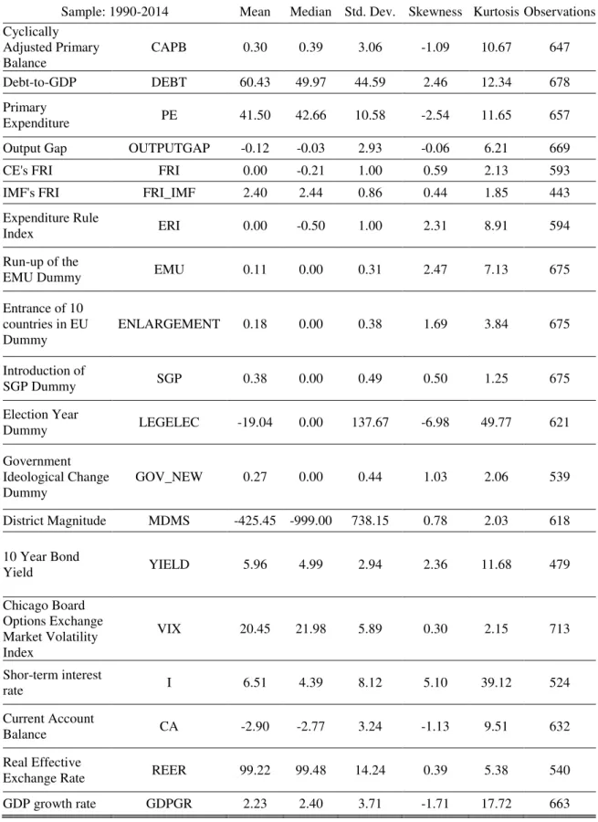
The statistical information as the number of observations, average and standard deviation
of all variables used in the empirical analysis can be found in Appendix B.
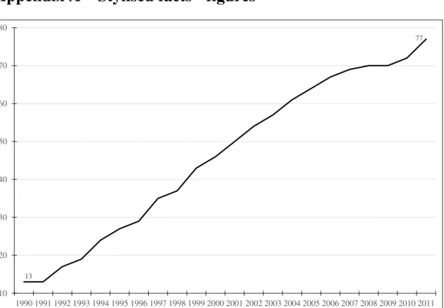
3.2. Stylised Facts
Based on EC’s FRI, the number of numerical fiscal rules in place since 1990 has
continuously grown from 13 rules to a total of 77 in 2011 (Figure A-I in Appendix A).
16
1990 to 2011, with debt rules and the expenditure rules in the recent years increasing
considerably. Rules targeting government revenue are the ones with less representation
(Figure A-II).
Concerning the type of government that is covered, most of the rules were applied to the
Local Government throughout the years, with a growing representation of rules applied
to the General Government, in recent years (Figure A-III in Appendix A).
Central Government applied mostly expenditure rules, whereas General Government and
Local Government targeted the budget balance (Table II).
Table II
Total numerical fiscal rules by type of government and aggregate targeted GG LG RG CG SS Multiple Total
BBR 15 18 6 5 5 6 55
DR 7 11 2 3 1 3 27
ER 5 0 1 14 3 8 31
RR 2 0 0 3 1 3 9
ER/BBR 0 0 0 0 0 2 2
Total 29 29 9 25 10 22 124
Note: BBR – Balance Budget Rule; DR – Debt Rule; ER – Expenditure Rule; RR
– Revenue Rule; GG – General Government; LG – Local Government ; RG –
Regional Government; SS – Social Security.
Source: Numerical Fiscal Rule Database, European Commission.
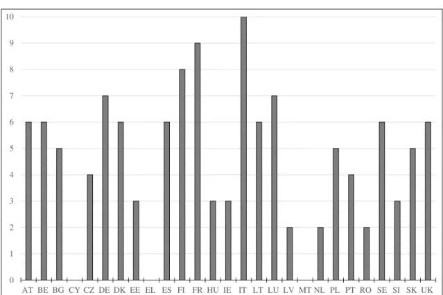
Currently, almost all EU countries have fiscal rules in place. Italy is the country with
more rules, ten, in the range of years considered (see Figure A-IV in Appendix A),
whereas the ones with less rules are Latvia, the Netherlands and Romania (Figure A-IV).
Cyprus, Greece and Malta never adopted a numerical fiscal rule. In 2011, the country
with more rules applied, six, was France (Figure A-V in Appendix A) and almost 30% of
the countries had only 2 rules in place.
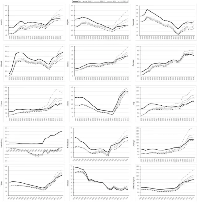
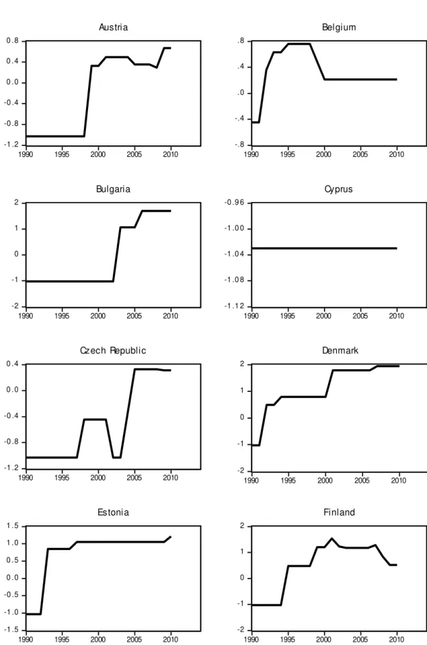
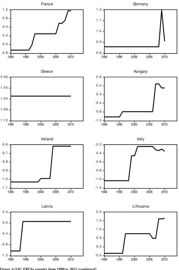
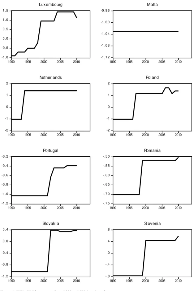
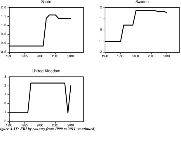
Analysing now the evolution of the FRI per country, we can see countries with no
variation in the way they implemented numerical fiscal rules, starting by the countries
17
Netherlands, Latvia, Romania, Germany that have changed their rules a few times, and
countries that are more dynamic with more frequent changes in the rules (Appendix A,
Figure A-VI to A-IX).
4.
Empirical Strategy and Results
4.1. Empirical specifications
For the empirical analysis, we use a fiscal reaction function to assess the impact of the
existence of fiscal rules on the primary balance (Debrun et al., 2008). Therefore, we have
estimated a fiscal reaction function following the common approach in the literature (see
Table I for a review of the literature on the subject):
𝑐𝑎𝑝𝑏𝑖𝑡 = 𝛽𝑖 + 𝛿𝑑𝑒𝑏𝑡𝑖𝑡−1+ 𝜆𝑜𝑢𝑡𝑝𝑢𝑡𝑔𝑎𝑝𝑖𝑡−1+ 𝜙𝑓𝑟𝑖𝑖𝑡+ 𝛾𝑥𝑖𝑡+ 𝑢𝑖𝑡. (1)
Where capbit is the cyclically adjusted primary balance in country i at time t, βi represents
the individual effects of each country i, debtit-1 is the debt-to-GDP ratio of country i in
period t-1, outputgapit-1 is the lagged output gap, friit is the fiscal rule index and finally xit
represents a set of variables that can have additional explanatory power, focusing on
specific events (e.g. election years and run-up to EMU).
After computing the results we expect ϕ > 0 meaning that more and better rules (better
FRI) impacts positively in the value of the CAPB leading to a healthier fiscal position.
As mentioned above, we will do this exercise using the FRI from the EC and compare
these results with the ones using the IMF’s FRI. In addition, and to assess the
effectiveness of expenditure rules we will compute an expenditure rule index based on
18
To have an additional assessment of the importance of numerical fiscal rules for
long-term government bond yields, we also estimate a specification to analyse the impact of
FRI on the 10-year maturity bond yields:
𝑦𝑖𝑒𝑙𝑑𝑖𝑡 = 𝛽𝑖𝑡+ 𝜌𝑋̅𝑖𝑡 + 𝜙𝑓𝑟𝑖𝑖𝑡+ 𝛾𝑣𝑖𝑥𝑖𝑡 + 𝜆𝐼𝑖𝑡+ 𝑢𝑖𝑡, (2)
where, 𝑦𝑖𝑒𝑙𝑑𝑖𝑡 is the 10-year maturity bond yield, 𝑋̅𝑖𝑡 is a vector comprising CAPB, debt,
CAB, REER, IP, GDPgr and CIP, for period t and country i. vixit is the measure of
investors’ willingness to take risk, Iit is the short-term interest rate for each period t and
county i and fri has the definition already mentioned above.
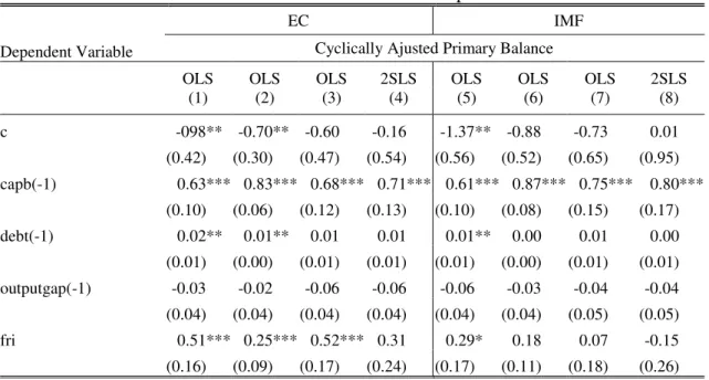
4.2. Baseline Results
Our baseline results for the EC index overall suggest that the FRI is significant with a
positive coefficient, this means that if the FRI increases by 1 unit, the CAPB can increase
up to 0.52 percentage points (p.p.). In column 1, Table III, the control variables were
omitted to see if they can bias the impact of the rules, and the effect is still robust.
Table III
Baseline results: fiscal rules and fiscal performance
EC IMF
Dependent Variable Cyclically Ajusted Primary Balance OLS
(1) OLS (2) OLS (3) 2SLS (4) OLS (5) OLS (6) OLS (7) 2SLS (8)
c -098 ** -0.70 ** -0.60 -0.16 -1.37 ** -0.88 -0.73 0.01 (0.42) (0.30) (0.47) (0.54) (0.56) (0.52) (0.65) (0.95) capb(-1) 0.63 *** 0.83 *** 0.68 *** 0.71 *** 0.61 *** 0.87 *** 0.75 *** 0.80 ***
19
EC IMF
Dependent Variable Cyclically Ajusted Primary Balance OLS
(1) OLS (2) OLS (3) 2SLS (4) OLS (5) OLS (6) OLS (7) 2SLS (8)
emu - 1.19 *** 2.05 *** 2.34 ** - 0.89 ** 3.89 *** 3.76 *** (0.31) (0.76) (1.06) (0.38) (0.80 ) (0.83) enlargement - 0.20 1.23 ** -1.30 *** - 0.25 0.49 1.05 (0.28) (0.48) (0.44) (0.34) (0.63) (0.70) sgp - -0.06 -0.87 * 1.30 ** - -0.13 -1.00 ** -1.01 **
(0.20) (0.44) (0.54) (0.21) (0.48) (0.57) legelec - -0.77 *** -0.72 *** -0.64 *** - -0.70 *** -0.72 *** -0.73 ***
(0.17) (0.17) (0.18) (0.18) (0.19) (0.20) gov_new - 0.43 ** 0.50 ** 0.59 ** - 0.52 ** 0.66 *** 0.75 ***
(0.20) (0.23) (0.25) (0.24) (0.25) (0.27) mdms - 0.00 0.00 0.00 ** - 0.00 0.00 * 0.00 **
(0.00) (0.00) (0.00) (0.00) (0.00) (0.00) Number of observations 463 437 437 397 420 366 366 324 R2 0.72 0.69 0.76 0.77 0.73 0.67 0.78 0.78
Adjusted R2 0.69 0.68 0.73 0.73 0.70 0.66 0.74 0.74
Endogeneity test - - - 0.21 - - - 0.74 Fixed Effects 1.97 *** - 2.16 *** - 2.55 *** - 2.05 *** - Random effects
(Hausman test)
Period - 20.66 ** - - 15.94 - - Cross-section - 13.40 - - 9.82 - - Notes: Robust standard errors are reported in parenthesis *, **, and *** denote, respectively, significance at the 10, 5 and 1% level. Period range for EC’s FRI: 1991-2011 (463 observations), 1991-2010 (437
observations and 397 observations). Period range for IMF’s FRI: 1990-2011 (420 observations), 1991-2010
(366 observations and 324 observations). Instrumental variables are the FRI own lag and a variable capturing the commitment of governments.
When the control variables are included in column (2), Table III, the run-up to the EMU,
the election period and the ideological change in government composition have a
significant impact on de dependent variable. The interpretation is as follows: in the years
of implementation of the EMU in the EU-15 countries, the CAPB is 1.19 p.p. higher. The
years where occurred an ideological change led to an increment of the CAPB of 0.43 p.p.
20
The results obtained from a fixed effects OLS regression, column (3), Table III, are
essentially the same, with two more variables becoming statistically significant, the
EU-10 countries after 2003 have an increment of 1.23 p.p on CAPB and those being part of
the euro-area after 1998 have a negative impact of CAPB of -0.87.
Column 4, Table III, reports a Two Stage Least Squares with the instrument of FRI being
its own lag and a variable capturing the commitment of governments2, FRI is no longer
significant and the p-value of the Wu-Hausman test shows that there are no problems of
endogeneity. However, there are concerns about reverse causality between the fiscal
stance and FRI, still, by analysing the Granger Causality Test (Appendix CTable C-III)
we cannot conclude if, in fact, is the implementation of fiscal rules that leads to better
balances, or if it is the better fiscal outcomes that lead to the implementation of more
rules.
The use of the IMF’s Fiscal Rule Index generates some different results, and for the same
period range we have only 366 observations. The index is significant only at a level of
10% with no control variables included. Although the index takes into account the same
characteristics and types of rules, the methodology used is different and so the results
might differ because of that (see column (5)-(8), Table III). Therefore, the methodology
used to compute the index may have an important role in the conclusions that can be made
about the impact of fiscal rules in fiscal outcomes.
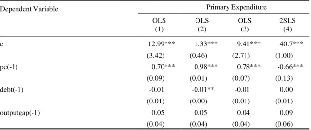
We performed the same exercise for the IMF Expenditure Rule Index (ERI), calculated
based on the methodology provided in the EC’s FRI Database applied only to rules
21
targeting public expenditure. We considered as dependent variable the Primary
Expenditure - interest payments are hardly controlled by the governments - as expenditure
rules are more effective regarding expenditure alone and not the whole balance (see Table
IV).
We performed again a fixed effects OLS regression and an IV estimation with the
instrument being the ERI’s own lag. Column (1), Table IV, similarly to the analysis for
the FRI, accounts for the possibility of control variables biased the significance of the
ERI on Primary Expenditure. Despite this omission, numerical expenditure rules
contribute to the control of public expenditure at a significant level. This conclusion is
valid when the control variables are included, column (2), but with a smaller coefficient.
In this way, holding everything constant, the increase of one unit in the ERI contributes
to a decrease of the Primary Expenditures-to-GDP ratio of 0.18 p.p. in (2) and 0.37 p.p.
in (3). The introduction of the SGP, election periods, and changes in government ideology
are other explanatory variables with an impact in Public Expenditure. The results remain
robust when the ERI instruments are used, confirming that the results are not biased due
to reverse causality.
Table IV
The impact of expenditure rules on primary expenditure
Dependent Variable Primary Expenditure
OLS
(1) OLS (2) OLS (3) 2SLS (4)
c 12.99 *** 1.33 *** 9.41 *** 40.7 ***
(3.42) (0.46) (2.71) (1.00)
pe(-1) 0.70 *** 0.98 *** 0.78 *** -0.66 ***
(0.09) (0.01) (0.07) (0.13)
debt(-1) -0.01 -0.01 ** -0.01 0.00
(0.01) (0.00) (0.01) (0.01)
outputgap(-1) 0.05 0.05 0.04 0.09
(0.04) (0.04) (0.04) (0.06)
22
Dependent Variable Primary Expenditure
OLS
(1) OLS (2) OLS (3) 2SLS (4)
eri -0.33 ** -0.18 ** -0.37 ** -0.88 ***
(0.15) (0.09) (0.16) (0.23)
emu - -0.44 * -1.47 -2.64
(0.25) (1.02) (1.65)
enlargement - -0.39 * -0.16 -0.58
(0.24) (0.46) (0.70)
sgp - 0.23 0.96 ** 2.59 ***
(0.18) (0.47) (0.67)
legelec - 0.63 *** 0.59 *** 0.62 **
(0.17) (0.16) (0.25)
gov_new - -0.41 ** -0.57 *** -0.77 ***
(0.19) (0.21) (0.29)
mdms - 0.00 0.00 0.00
(0.00) (0.00) (0.00)
Number of observations 464 437 437 397
R2 0.98 0.97 0.98 0.97
Adjusted R2 0.97 0.97 0.97 0.96
Endogeneity test - - - 0.11
Fixed Effects 2.56 *** 1.54 **
Random effects (Hausman test)
Period - 17.88 * - -
Cross-section - 33.09 *** - -
Notes: Robust standard errors are reported in parenthesis *, **, and *** denote, respectively, significance at the 10, 5 and 1% level. Period range: 1991-2011 (464 observations), 1991-2010 (437 observations and 397 observations). Instrumental variables are the ERI own lag and a variable capturing the commitment of governments.
To stress the importance of numerical fiscal rules, we performed an additional empirical
exercise to assess the impact of rules on the 10-year maturity bonds yield. The index
shows significance in every regression computed, meaning that if the FRI increases by
one unit, the yield, in (1) of Table V, decreases by 0.25 p.p. When investors become more
risk averse - vix increases - we can see that, holding everything else constant, the yields
decrease by 0.02 p.p.. As expected, the variables representing better economic
23
(3) of Table V, we performed a 2SLS, the endogeneity testes shows that the FRI is not
endogenous, regarding causality, the Granger tests in Appendix C, show that causality
runs from the FRI to the yields.
In Appendix C, Table C-I and Table-CII, it is possible to observe regression results
considering different sets of explanatory variables and, also, the same regressions but
considering the yield spread against Germany as the dependent variable. The conclusions
are the same, the FRI is significant in all regressions and the variables capturing economic
developments maintain their statistical significant as well.
Table V
The impact of FRI on 10-Year Bond Yield Dependent Variable 10 year bond yield
OLS
(1) OLS (2) 2SLS (3)
c 6.44 *** 7.57 *** 6.25 ***
(1.02) (0.92) (0.82) capb(-1) -0.13 *** -0.15 *** -0.14 ***
(0.03) (0.03) (0.03)
debt 0.00 0.01 * 0.00
(0.00) (0.01) (0.00)
cpi 0.01 -0.02 * 0.01
(0.01) (0.01) (0.01)
cab 0.02 0.08 *** 0.03
(0.02) (0.03) (0.02)
reer 0.00 - -
(0.01)
i 0.53 *** 0.47 *** 0.51 ***
(0.04) (0.04) (0.03) ip -0.04 *** -0.02 *** -0.03 ***
(0.01) (0.01) (0.01) fri -0.25 *** -0.30 *** -0.34 ***
(0.07) (0.11) (0.10) vix -0.02 -0.02 * -0.02 **
(0.01) (0.01) (0.01) gdpgr -0.10 ** -0.13 *** -0.10 **
24
Dependent Variable 10 year bond yield
OLS
(1) OLS (2) 2SLS (3) Number of observations 337 362 335
R2 0.63 0.75 0.68
Adjusted R2 0.62 0.72 0.68
Endogeneity test - - 0.36 Cross-section fixed effects - 3.33 *** - Random effects
(Hausman test)
Cross-section 56.78 *** - - Notes: Robust standard errors are reported in parenthesis *, **, and *** denote, respectively, significance at the 10, 5 and 1% level. Period range: 1995-2011 (337 observations), 1991-2010 (362 observations and 335 observations). Instrumental variables are the FRI own lag and a variable capturing the commitment of governments.
Overall, we observe that the FRI is strongly significant is most of the regressions, together
with the variables capturing developments in the EU and in the EMU (sgp, emu, and
enlargement). The variables capturing countries specific developments – election and
gov-new – have also explanatory power for the budget balances. When we consider only
expenditure rules, these are also important to explain primary expenditure ratios.
Countries with rules applied to discretionary public expenditure experience better
expenditure ratios. In addition, capital markets react positively to countries that have rules
implemented, demanding lower yields.
4.3. Simulation
Finally, we performed a simulation of the level of government debt, by computing an expenditure
rule and applying it to the real expenditure level based on the specifications in Hauptmeier et al.
25
The simulation exercise has the purpose of understanding what would have been the debt
developments if EU countries had adopted a rule for the discretionary component of public
expenditures.
First, we have a few countries with an unusual situation in the period considered, with
years where public expenditures were greater than the consolidated gross debt. For that
reason, rule-based expenditure levels would lead to negative values of debt.
Second, in the majority of the countries only when GDP was computed considered an
expenditure multiplier of 0.3 the debt ratio was lower than the actual ratio, considering
the last five year of the analysis. In 2013, only three countries do not present rule-based
values of the debt ratio above the actual one: Italy, Greece and Sweden. Sweden is the
only case, in the EU-15 countries that would not benefit of a ruled-based expenditure
path, with new debt developments very similarly to the actual path.
Considering the SGP constraint of maintaining the debt ratio below 60%, this barrier
would have been exceed much later, for Denmark this means that it would never
experience debt ratios above 60%. For Austria, instead of being over 60% in 1993 it
would only reach this value in 2009, as well as France and Portugal, instead of 2003 and
2004, respectively. Greece would not enter the EMU and adopted the SGP with debt ratios
already above 60% but would pass it only in 1996, the barrier of 100% debt would only
be achieved in 2009 instead of 1996.
Overall, the fiscal stance of the majority of EU countries would have been much sounder
26
27
5.
Conclusions
The purpose of this thesis was to assess whether countries with more or better fiscal rules
implemented have better budget balances, and consequently better debt ratios. From the
theory discussed, the general idea is that there is a relation between fiscal rules and fiscal
balances. From our empirical study we confirm that countries with more fiscal rules, in
fact, have better CAPB. But we could not guarantee that causality runs from FRI to
CAPB. Also, the methodology used to compute this type of indexes seems to matter,
given that IMF’s FRI for the same countries, considering broadly the same criteria,
produces different results from the ones computed with the EC’s FRI.
Considering the capital markets perspective, we studied the impact of the FRI on the
10-year bond yield. Investors seem to reward countries that have implemented fiscal rules,
and this can be explained by the commitment associated with such rules and with more
certainty about the fiscal results.
With revenues being essential a-cyclical, we tried to prove that rules applied to public
expenditures contribute to their control and for the consolidation of fiscal balances, our
regression results show that the ERI has explanatory power to explain developments in
primary expenditures. Therefore, it is justifiable to construct rules that target specifically
the expenditure side of budget.
This leads to the second objective of our work, assess the debt developments of the EU
countries if they had implemented an expenditure rule in 1990. If public expenditures had
increased at the growth rate of potential GDP, countries would have experienced smaller
debt ratios compared to the actual ones and would have had more easily complied with
28
As mentioned before, this work has some limitations. First, it was not possible to prove
that, without doubt, the FRI causes better results of the CAPB and not the other way
around. Second, different methods of computing the fiscal rule index can lead to different
results. Further analysis on the proper methodology to be used or new instruments
capturing the commitment to rules could contribute to the conclusions on the subject.
29
References
Afonso, A., & Hauptmeier, S. (2009). Fiscal behaviour in the European Union - rules, fiscal decentralization and government indebtedness, ECB Working Paper Series, 1054.
Annett, A. (2006). Enforcement and the Stability and Growth Pact: How Fiscal Policy Did and Did Not Change Under Europe’s Fiscal Framework, IMF Working Papers, 06/116.
Ayuso, J. (2012). National Expenditure Rules – Why, How and When, EC Economic Papers, 473.
Ayuso, J., Debrun, X., Kumar, M. S., Moulin, L., & Turrini, A. (2007). Beyond the SGP - Features and effects of EU national-level numerical fiscal rules, Centre for Economic Policy Research.
Baum, A., Ribeiro, M. P., & Weber, A. (2012). Fiscal Multipliers and the State of the Economy, IMF Working Papers, 12/286.
Boussard, J., de Castro, F., & Salto, M. (2012). Fiscal Multipliers and Public Debt Dynamics in Consolidations, Directorate General Economic and Monetary Affairs (DG ECFIN), European Commission.
Budina, N., Schaechter, A., Weber, A., & Kinda, T. (2012). Fiscal Rules in Response to the Crisis - Toward the "Next-Generation" Rules. A New Dataset, IMF Working Papers, 12/187.
Debrun, X., Moulin, L., Turrini, A., Ayuso-i-Casals, J., & S. Kumar, M. (2008). Tied to the mast? National fiscal rules in the European Union. Economic Policy, 23, 297-362.
European Commission. (2008). Fiscal rules in the EU at national level : experiences and lessons.
Presupuesto y gasto público, 51(2), p.59-82.
Gali, J., & Perotti, R. (2003). Fiscal Policy and Monetary Integration in Europe. Economic Policy, 18(37), 533-572.
Hallerberg, M., Strauch, R., & Hagen, J. v. (2009). Fiscal Governance in Europe.
Hauptmeier, S., Sanchez-Fuentes, J., & Schuknecht, L. (2010). Towards expenditure rules and fiscal sanity in the euro area. 1266.
Holm-Hadulla, F., Hauptmeier, S., & Rother, P. (2010). The impact of numerical rules on budgetary discipline over the cycle, ECB Working Paper Series, 1169.
Klaus Armingeon, R. C., David Weisstanner, Sarah Engler, Panajotis Potolidis, Marlène Gerber. (2012). Comparative Political Data Set III (35 OECD Countries and/or EU-member countries).
Kopits, G., & Symansky, S., A. (1998). Fiscal Policy Rules, IMF Occasional Papers, 162.
Kumar, M., Baldacci, E., Schaechter, A., Caceres, C., Kim, D., Debrun, X., . . . Zymek, R. (2009). Fiscal Rules - Anchoring Expectations for Sustainable Public Finances, IMF staff paper. Pina, Á. M., & Venes, N. M. (2011). The political economy of EDP fiscal forecasts: An empirical
assessment. European Journal of Political Economy, 27(3), 534-546.
Schuknecht, L. (2004). EU fiscal rules: issues and lessons from political economy, ECB Working Paper Series, 421.
Turrini, A. (2008). Fiscal policy and the cycle in the Euro Area: The role of the government revenue and expenditure. European Economy - Economic Papers, 323.
30
Appendix A
–
Stylised facts - figures
13
77
10 20 30 40 50 60 70 80
1990 1991 1992 1993 1994 1995 1996 1997 1998 1999 2000 2001 2002 2003 2004 2005 2006 2007 2008 2009 2010 2011
Figure A-I: Evolution of total number of rules from 1990 to 2011
0 10 20 30 40 50 60 70 80
1990 1991 1992 1993 1994 1995 1996 1997 1998 1999 2000 2001 2002 2003 2004 2005 2006 2007 2008 2009 2010 2011 BBR DR ER RR ER/BBR
31 0
1 2 3 4 5 6 7 8 9 10
AT BE BG CY CZ DE DK EE EL ES FI FR HU IE IT LT LU LV MT NL PL PT RO SE SI SK UK 0
10 20 30 40 50 60 70 80
1990 1991 1992 1993 1994 1995 1996 1997 1998 1999 2000 2001 2002 2003 2004 2005 2006 2007 2008 2009 2010 2011 GG LG RG CG SS Multiple
Figure A-IV: Total numerical fiscal rules by country
32 0
1 2 3 4 5 6
AT BE BG CY CZ DE DK EE EL ES FI FR HU IE IT LT LU LV MT NL PL PT RO SE SI SK UK
33
-1 .2 -0 .8 -0 .4 0 . 0 0 . 4 0 . 8
1990 1995 2000 2005 2010
Austria -.8 -.4 . 0 . 4 . 8
1990 1995 2000 2005 2010
Belgium -2 -1 0 1 2
1990 1995 2000 2005 2010
Bulgaria
-1 .1 2 -1 .0 8 -1 .0 4 -1 .0 0 -0 .9 6
1990 1995 2000 2005 2010
Cyprus
-1 .2 -0 .8 -0 .4 0 . 0 0 . 4
1990 1995 2000 2005 2010
Czech Republic
-2 -1 0 1 2
1990 1995 2000 2005 2010
Denmark
-1 .5 -1 .0 -0 .5 0 . 0 0 . 5 1 . 0 1 . 5
1990 1995 2000 2005 2010
Estonia -2 -1 0 1 2
1990 1995 2000 2005 2010
Finland
34
-0 .8 -0 .4 0 . 0 0 . 4 0 . 8 1 . 2
1990 1995 2000 2005 2010
France
0 . 8 0 . 9 1 . 0 1 . 1 1 . 2
1990 1995 2000 2005 2010
Germany
-1 .1 2 -1 .0 8 -1 .0 4 -1 .0 0 -0 .9 6
1990 1995 2000 2005 2010
Greece
-1 .2 -0 .8 -0 .4 0 . 0 0 . 4 0 . 8
1990 1995 2000 2005 2010
Hungary -1 .1 -1 .0 -0 .9 -0 .8 -0 .7 -0 .6
1990 1995 2000 2005 2010
Ireland -1 .2 -1 .0 -0 .8 -0 .6 -0 .4 -0 .2
1990 1995 2000 2005 2010
Italy
-1 .2 -0 .8 -0 .4 0 . 0 0 . 4
1990 1995 2000 2005 2010
Latvia
-0 .5 0 . 0 0 . 5 1 . 0 1 . 5 2 . 0
1990 1995 2000 2005 2010
Lithuania
35
-1 .0 -0 .5 0 . 0 0 . 5 1 . 0 1 . 5
1990 1995 2000 2005 2010
Luxembourg
-1 .1 2 -1 .0 8 -1 .0 4 -1 .0 0 -0 .9 6
1990 1995 2000 2005 2010
Malta -2 -1 0 1 2
1990 1995 2000 2005 2010
Netherlands -2 -1 0 1 2
1990 1995 2000 2005 2010
Poland -1 .2 -1 .0 -0 .8 -0 .6 -0 .4 -0 .2
1990 1995 2000 2005 2010
Portugal -.7 5 -.7 0 -.6 5 -.6 0 -.5 5 -.5 0
1990 1995 2000 2005 2010
Romania
-1 .2 -0 .8 -0 .4 0 . 0 0 . 4
1990 1995 2000 2005 2010
Slovakia -.8 -.4 . 0 . 4 . 8
1990 1995 2000 2005 2010
Slovenia
36
-0 .5 0 . 0 0 . 5 1 . 0 1 . 5 2 . 0
1990 1995 2000 2005 2010
Spain
-2 -1 0 1 2
1990 1995 2000 2005 2010
Sweden
-2 -1 0 1 2 3
1990 1995 2000 2005 2010
United Kingdom
37
Appendix B
–
Data statistics
Table B-I Descriptive statistics
Sample: 1990-2014 Mean Median Std. Dev. Skewness Kurtosis Observations Cyclically
Adjusted Primary
Balance CAPB 0.30 0.39 3.06 -1.09 10.67 647 Debt-to-GDP DEBT 60.43 49.97 44.59 2.46 12.34 678 Primary
Expenditure PE 41.50 42.66 10.58 -2.54 11.65 657 Output Gap OUTPUTGAP -0.12 -0.03 2.93 -0.06 6.21 669 CE's FRI FRI 0.00 -0.21 1.00 0.59 2.13 593 IMF's FRI FRI_IMF 2.40 2.44 0.86 0.44 1.85 443 Expenditure Rule
Index ERI 0.00 -0.50 1.00 2.31 8.91 594
Run-up of the
EMU Dummy EMU 0.11 0.00 0.31 2.47 7.13 675
Entrance of 10 countries in EU
Dummy ENLARGEMENT 0.18 0.00 0.38 1.69 3.84 675
Introduction of
SGP Dummy SGP 0.38 0.00 0.49 0.50 1.25 675
Election Year
Dummy LEGELEC -19.04 0.00 137.67 -6.98 49.77 621
Government Ideological Change
Dummy GOV_NEW 0.27 0.00 0.44 1.03 2.06 539
District Magnitude MDMS -425.45 -999.00 738.15 0.78 2.03 618
10 Year Bond
Yield YIELD 5.96 4.99 2.94 2.36 11.68 479
Chicago Board Options Exchange Market Volatility Index
VIX 20.45 21.98 5.89 0.30 2.15 713
Shor-term interest
rate I 6.51 4.39 8.12 5.10 39.12 524
Current Account
Balance CA -2.90 -2.77 3.24 -1.13 9.51 632
Real Effective
38
Appendix C
–
Additional Results
Table C-I
Estimation results considering the impact of FRI on 10 Year Bond Yield Dependent Variable 10 year bond yield
OLS
(1) OLS (2) 2SLS (3) c 5.89 *** 5.77 *** 5.66 ***
(1.04 ) (1.20 ) (1.07) capb(-1) -0.04 - -0.03 (0.03 ) (0.04)
debt 0.00 - 0.00)
(0.00 ) (0.00)
cpi 0.02 ** 0.02 ** 0.03 **
(0.01 ) (0.01 ) (0.01)
cab 0.01 0.00 0.01
(0.02 ) (0.02 ) (0.03)
reer 0.00 0.00 0.00
(0.01 ) (0.01 ) (0.01) i 0.54 *** 0.53 *** 0.53 ***
(0.04 ) (0.04 ) (0.04) ip -0.04 *** -0.03 *** -0.03 ***
(0.01 ) (0.01 ) (0.01) fri -0.30 *** -0.32 *** -0.42 ***
(0.07 ) (0.07 ) (0.10) vix -0.03 *** -0.03 ** -0.04 ***
(0.01 ) (0.01 ) (0.01) gdpgr -0.12 *** -0.13 *** -0.12 ***
(0.04) (0.04) (0.05) Number of observations 338 338 311
R2 0.60 0.59 0.60
Adjusted R2 0.59 0.58 0.59
Endogeneity test - - 0.01 Random effects
39 Table C-II
Estimation results considering the impact of FRI on 10-Year Yield Spreads against Germany
Dependent Variable 10-year yield spread against Germany
OLS (1) OLS (2) 2SLS (3) OLS (4) OLS (5) 2SLS (6)
c -2.46 ** -2.68 ** -2.74 *** c -1.92 ** -0.65 -3.68 *** (0.98) (1.16) (1.03) (0.96) (0.73) (0.78) capb -0.06 * - -0.05 capb(-1) -0.15 *** -0.14 *** -0.16 ***
(0.03) (0.04) (0.03) (0.03) (0.03) debt 0.00 - 0.00 debt 0.00 0.02 *** 0.00 (0.00) (0.00) (0.00) (0.01) (0.00) cpi 0.09 *** 0.09 *** 0.09 *** cpi 0.07 *** 0.02 ** 0.06 ***
(0.01) (0.01) (0.01) (0.01) (0.01) (0.01) cab 0.00 -0.01 0.00 cab 0.02 0.10 *** 0.03 (0.02) (0.02) (0.03) (0.02) (0.02) (0.02) reer -0.02 *** -0.02 ** -0.02 ** reer -0.02 ** - -
(0.01) (0.01) (0.01) (0.01)
i 0.42 *** 0.41 *** 0.41 *** i 0.41 *** 0.27 *** 0.34 *** (0.03) (0.03) (0.04) (0.03) (0.03) (0.04) ip -0.03 *** -0.03 *** -0.03 *** ip -0.03 *** -0.02 ** -0.02 **
(0.01) (0.01) (0.01) (0.01) (0.01) (0.01) fri -0.28 *** -0.32 *** -0.37 *** fri -0.23 *** 0.09 -0.19 **
(0.07) (0.07) (0.09) (0.06) (0.09) (0.10) vix -0.04 *** -0.04 *** -0.04 *** vix -0.02 * -0.02 -0.01 (0.01) (0.01) (0.01) (0.01) (0.01) (0.01) gdpgr -0.12 *** -0.13 *** -0.12 ** gdpgr -0.10 ** -0.12 *** -0.08 *
(0.04) (0.04) (0.05) (0.04) (0.04) (0.04) Number of observations 338 338 311 337 362 335
R2 0.57 0.56 0.57 0.62 0.73 0.54
Adjusted R2 0.56 0.55 0.56 0.61 0.70 0.53
Endogeneity test - - 0.08 - - 0.99
Cross-section fixed effects - - - - 8.60 *** -
Random effects
(Hausman test) - - - - - -
40 Table C-III Granger Causality
Null Hypothesis: Obs F-Statistic Prob.
41
Appendix D
–
Simulation Methodology and Figures
The methodology of the simulation exercise is based on Hauptmeier et al. (2010). The
first step is to construct a new expenditure path that follows a predetermined rule of
growth. For the purpose of this exercise we define the rule growth rate as the same growth
rate of potential GDP. The formulas needed are defined as follows:
Table D-I Simulation’s Methodology
Concept Formula
Expenditure path
𝐺𝑡 = 𝐺𝑡−1∗ (1 + 𝑔𝑟𝑡), 𝐺𝑡 = 𝐺𝑡 𝑤ℎ𝑒𝑛 𝑡 = 0
𝐺𝑡 is the rule-based expenditure path.
𝐺𝑡 is the actual expenditure path.
𝑔𝑟𝑡 is the growth rule
Debt path ∆𝐺𝑡 is the difference between the rule-based expenditure path and the actual 𝐷𝑡 = 𝐷𝑡+ ∆𝐺𝑡+ 𝐼𝑡, where expenditure path.
Interest rate r is the implicit interest rate computed as Interests over Gross Consolidated 𝐼𝑡 = ∆𝐺𝑡∗ 𝑟, Debt at period t.
GDP
𝑌𝑡 = 𝑌𝑡∗ (1 + %∆𝐺𝑡∗ 𝑚),
%∆𝐺𝑡 is the difference between the rule-based expenditure path and the actual
expenditure path in percentage of GDP, m is the expenditure multiplier – we consider four possible values 0.3, 0.75, 1, 1.53.
We used total expenditure excluding interest, consolidated gross debt, gdp at market prices all expressed in billions of national currency for each country extracted from AMECO Database.
3 GDP was computed considering different values for the impact of expenditure on output. The range used
42
43
44
45
46
47
48
49
50
51 Table D-II
52 Table D-III