INSTITUTO SUPERIOR DE ECONOMIA E GEST ˜

(1)

UNIVERSIDADE DE LISBOA

INSTITUTO SUPERIOR DE ECONOMIA E GEST ˜

AO

On the Sparre–Andersen risk model with different

type of interclaim times distributions

Agnieszka Izabella Bergel

Disserta¸cão para obten¸cão do Grau de Doutor em Matemática Aplicada à Economia e Gestão

Orientador:

Doutor Alfredo Duarte Eg´ıdio dos Reis

J´uri das provas de doutoramento Presidente: Reitor da Universidade de Lisboa

Vogais:

Doutora Maria de Lourdes Centeno Doutor Rui Manuel Rodrigues Cardoso Doutor Alfredo Duarte Eg´ıdio dos Reis Doutor St´ephane Loisel

(2)

(3)

(4)

(5)

Acknowledgements

During all those years of hard work on this Ph.D., hard thinking and time spent waiting for good ideas, developing them, or failing in the process, what I find the hardest is writing this thesis. I found myself staring at blank pages at the beginning of the writing process, looking for an inspiration that was coming only little by little.

There were many people, who supported me during my doctoral studies. The first person to mention is my supervisor Professor Alfredo Egidio dos Reis, I am grateful for his support, insightful corrections, comments, clarifica-tions, valuable guidance and especially for his friendship during these years. Thank you for having accepted me as a Ph.D. student and for believing in me. I am grateful to CEMAPRE - the Centre for Applied Mathematics and Economics for the financial support to present parts of this work at the Mem-orable Actuarial Research Conference 2011, the 15th and 16th Congresses on Insurance: Mathematics and Economics in 2011 and 2012 respectively, the ASTIN 2012 and 2013 conferences, and Sixth Brazilian Conference on Sta-tistical Modelling in Insurance and Finance in 2013. Participation in those conferences gave me opportunity to meet extraordinary people from whom I have learnt so many things, I’ve increased my knowledge in so many different areas.

I am very grateful to my committee, who will read this manuscript, for all the support they can provide in improving this work.

(6)

(7)

Resumo

Nesta disserta¸cão trabalhamos com teoria do risco, com especial ênfase sobre dois grandes temas da área, nomeadamente, os modelos de risco e a teoria de ru´ına. A resolu¸cão de equa¸cões é uma parte fundamental da matemática e de praticamente qualquer outra ciência. Muito frequentemente somos con-frontados com equa¸cões que foram formuladas pela observa¸cão da natureza durante a resolu¸cão de problemas relacionados aos fenómenos que ocorrem na vida real. Em ciências atuariais formulamos modelos de risco, a fim de resolver problemas que surgem na prática atuarial dos seguros.

Em muitas ocasiões, durante a análise de tais modelos, encontramos a equa¸cão de Lundberg. Há uma razão para isso: quando estudamos algumas quantidades espec´ıficas, como a probabilidade de ru´ına, chegamos frequente-mente a equa¸cões integro–diferenciais. Tais equa¸cões têm associado algum tipo de equa¸cão caracter´ıstica a que chamamos equa¸cão de Lundberg.

Neste tese, consideramos o modelo de risco Sparre–Andersen, com três diferentes distribui¸cões de tempo: Erlang(n), Erlang(n) generalizada e Phase–Type(n). Para cada um destes casos, a equa¸cão de Lundberg é difer-ente e, consequdifer-entemdifer-ente, é analisada de um modo único.

Depois, para cada distribui¸cão, estudamos alguns dos mais importantes tópicos de interesse neste modelo, como a ru´ına e as probabilidades de sobre-vivência, a probabilidade de atingir uma barreira superior antes da ru´ına, a gravidade máxima da ru´ına e os dividendos descontados esperados. O obje-tivo desta tese é fornecer novas ferramentas para calcular essas quantidades e uma melhor compreensão delas na prática.

(8)

(9)

Abstract

In this dissertation we work with risk theory with particular emphasis on two major topics in the field, namely risk models and ruin theory. Solving equa-tions is a fundamental part of mathematics and of almost any other science. Very often we come across equations that were formulated by observation of the nature, during solving problems related to phenomena that occur in life. In actuarial science, we formulate risk models in order to solve problems that appear in the practice of the insurance business.

Lundberg’s equations shows up on many occasions when analyzing such models. There is a reason for this: when we study some particular quantities like, for example, the ruin probability, we often arrive to integro–differential equations. Such integro–differential equations have associated some kind of characteristic equation. The latter is often called the Lundberg’s equation.

In this manuscript we consider the Sparre–Andersen risk model with three different interclaim times distributions: Erlang(n), generalized Erlang(n) and Phase–Type(n). For each of these cases the Lundberg’s equation is different and therefore it is analyzed in a unique way.

Afterwards, for each distribution, we study some of the most important topics of interest, like the ruin and survival probabilities, the probability of attaining and upper barrier prior to ruin, the maximum severity of ruin and the expected discounted dividends. The aim of this thesis is to provide new tools for computation of those quantities and a better understanding of them in the practice. In the process we give examples to illustrate those methods.

(10)

List of Symbols

B(D) differential operator

C.D.F. cumulative distribution function

J(z;u) distribution of the maximum severity of ruin

L.T. Laplace transform

Mu maximum severity of ruin

N(t) counting process

R adjustment coefficient

S(t) aggregate claims process

Tr an operator w.r.t. a complex number r

Tu time of ruin

V(u, b) expected present value of discounted dividends

Vm(u, b) m–th moment of discounted dividends

Wi interclaim timei

Xi claim amounti

Φ(u) survival probability Ψ(u) ruin probability

χ(u, b) probability of attaining the barrier levelb from initial surplus u

ˆ

h(s) Laplace transform of h

I₍_A₎ _{the indicator function of the set} _A

D differentiation with respect tou

I identity operator

c premium income

i.i.d. independent and identically distributed

k(t) density of interclaim times

p(x) density of claim amounts

(11)

List of Tables

3.1 Expected values and standard deviations of Mu for n= 1,2,3

(interclaim times) and m= 1 (claim amounts) . . . 38 3.2 Probability that the maximum deficit occurs at ruin, forn= 3,

m = 1. . . 39 3.3 Values of E(Mu) and s.d.(Mu) forn = 2;m = 1 andn=m= 2 42

3.4 Probability that the maximum deficit occurs at ruin, forn= 2,

(15)

List of Figures

2.1 The surplus process . . . 11

2.2 The time of ruin . . . 12

2.3 The net profit condition . . . 13

2.4 The time to attain the level b . . . 19

2.5 The maximum severity of ruin . . . 22

2.6 The expected discounted dividends . . . 25

2.7 The modified surplus . . . 26

(16)

Chapter 1 Introduction

If people do not believe that mathematics is simple, it is only because they do not realize how complicated life is

John von Neumann

Risk theory is a field of mathematics which has its origins in the beginning of twentieth century, when fundamental ideas were published by Lundberg (1903). Risk theory is a synonym for non–life insurance mathematics, which deals with the modeling of claims that arrive in an insurance business and which give insight on how much a premium has to be charged in order to avoid bankruptcy (ruin) of an insurance company. It is based on probability theory, statistics, stochastic processes, renewal theory, functional analysis and optimization theory, and investigates fluctuations shown by incoming claims at an insurance company. Claims are amounts of money to be paid to policy holders, and they are thought to be of uncertain size and coming at uncertain future instants. One of the Lundberg’s main contributions is the introduction of a simple model which is capable of describing the basic dynamics of a homogeneous insurance portfolio. By this we mean a portfolio of contracts orpolicies for similar risks such as car insurance for a particular kind of car, insurance against theft in households or insurance against water damage of family homes. There are three assumptions in the model:

• Claims happen at the times Ti satisfying 0 ≤T1 ≤ T2 ≤ · · ·. We call

them claim arrivals, claim times or claim arrival times.

• Thei–th claim arriving at timeTi causes the claim size or claim severity

Xi. The sequence {Xi} constitutes an i.i.d. sequence of non–negative

(17)

• The claim size process {Xi} and the claim arrival process {Ti} are

mutually independent.

Moreover, Risk theory has been an active research area in Actuarial Sci-ence since the 20th century. The heart of risk theory is ruin theory, which discusses how an insurance portfolio may be expected to vary with time. Ruin is said to occur if the insurer’s surplus drops under a specific lower bound. The probability that ruins occurs, commonly referred as the ruin probability, is a very important measure of risk.

Much of the literature on ruin theory is concentrated on the classical risk theory, where an insurer starts with an initial surplus u, collects premiums continuously at a constant rate ofc, while the aggregate claim process follows a compound Poisson process. The main research interest is the calculation of finite and infinite time ruin probabilities. Later on, actuarial researchers considered more components related to the time of ruin, like the surplus prior to ruin, the severity or deficit at ruin and its maximum, the probability of attaining a given upper barrier before ruin and the expected discounted dividends. Many results involving those quantities have been found during the recent years.

Gerber and Shiu (1998) considers the evaluation of the expected dis-counted penalty function, giving a unified treatment to the surplus before ruin, the deficit at ruin and the time to ruin.

Great part of the results in the classical risk model, like the results of Gerber et al. (1987), Dufresne and Gerber (1988a), Dufresne and Gerber (1988b), Dickson (1992) and Dickson and Eg´ıdio dos Reis (1996), are ob-tained as particular cases when the discount factor is zero, and almost all the previous results in classical ruin theory can be extended to the case with a positive discounting factor.

Lin and Willmot (1999) proposed an approach to solve the defective re-newal equation, in which the discounted penalty function is expressed in terms of a compound geometric tail. Lin and Willmot (2000) further used it to derive the moments of the surplus before ruin, the deficit at ruin and the time of ruin.

(18)

Sparre-Andersen (1957) in a paper to the International Congress of Ac-tuaries in New York proposed a generalization of the classical (Poisson) risk theory, instead of assuming just exponentially distributed independent inter– occurrence (interclaim) times, he introduced a more general distribution function but retained the assumption of independence. He let claims occur according to a more general renewal process and derived an integral equa-tion for the corresponding ruin probability. Since then the Sparre–Andersen model has been studied by many authors. In addition, random walks and queueing theory have provided a more general framework, which has led to explicit results in the case where the waiting times or the claim severities have distributions related to the Erlang (see Borovkov (1976)).

Malinovskii (1998) gives the Laplace transform of the non-ruin probability as a function of a finite time t, if claim sizes are exponentially distributed with parameter α, and waiting times have a general distribution k. Wang and Liu (2002) extends the result to claim sizes that are mixture of two exponential distributions.

Dickson (1998) and Dickson and Hipp (1998) showed how methods that are applied to derive results for the classical risk process can be adapted to derive results for a class of risk process in which the claims occur as a renewal process, namely as an Erlang(2) process. Dickson and Hipp (2001) considered a Sparre–Andersen risk process for which the interclaim times distribution is Erlang(2) with the purpose to find expressions for moments of the time of ruin, given that ruin occurs. They obtain an explicit expression for the Laplace transform of the ruin probability by solving a second order integro– differential equation. More recently, Cheng and Tang (2003) complements the work of Dickson and Hipp (2001), discussing the moments of the surplus before ruin and the deficit at ruin in the Erlang(2) risk process.

Li and Garrido (2004b) extended the Erlang(2) risk model to Erlang(n) for any integer n. They studied the joint distribution of the time of ruin, the surplus just before ruin and the deficit at ruin and proved that the ex-pected discounted penalty function satisfies ann-th order integro–differential equation. The latter can be solved to obtain a defective renewal equation. Li and Garrido (2004a), Gerber and Shiu (2005), Gerber and Shiu (2003a) and Gerber and Shiu (2003b) further extend the Erlang risk models to gen-eralized Erlangs, in which interclaim times are distributed as the sum of n

(19)

initial surplus and the given level, satisfied a homogeneous integro–differential equation with certain boundary conditions. Its solution was expressed as a linear combination of n linearly independent particular solutions of the homogeneous integro–differential equation.

Li (2008), continuing this approach, studied the distributions of the max-imum surplus before ruin and the maxmax-imum severity of ruin for an Erlang(n) risk model, and showed a method to find the particular solutions of the ho-mogeneous integro–differential equation using the roots of the generalized Lundberg’s equation.

Dickson and Waters (2004) considered a surplus process modified by the introduction of a constant dividend barrier, which was originally proposed by de Finetti (1957), and extended some results relating to the distribution of the present value of dividend payments until ruin in the classical risk model and show how a discrete time model can be used to provide approximations when analytic results are not available. Later on Albrecher et al. (2005) continued the work on dividends for a Sparre–Andersen risk model with generalized Erlang(n) distributed interclaim times and a constant dividend barrier.

Some authors have studied the Sparre–Andersen risk model with Phase– Type interclaim times. Ren (2007) studied this risk model deriving a matrix form expression for the discounted joint density of the surplus prior to ruin and the deficit at ruin when the initial surplus is zero. Li (2008b) analyzed some quantities like the Laplace transform of the recovery time after ruin, the probability that the surplus attains a certain level before ruin and the distribution of the maximum severity of ruin. Ji and Zhang (2011) analyzed the role of the distinct roots of the fundamental Lundberg’s equation in the right half of the complex plane and the linear independence of the eigenvec-tors related to the Lundberg’s matrix.

Willmot (1999) considers the ruin probabilities for renewal risk processes where the waiting times have a Kn distribution, for which the associated

Laplace–Stieltjes transform is the ratio of a polynomial of degree m < n to a polynomial of degree n. This general class of distributions includes, as special cases, Erlang and Phase–Type distributions, as well as combinations of these.

Stanfordet al.(2000) presents a recursive method of calculating ruin prob-abilities for non–Poisson risk processes, by looking at the surplus process embedded at claim instants, in which interclaim times are assumed to be mixtures of exponential and Erlang(n) distributions.

(20)

admit a rational Laplace transform representation. Lima et al. (2002) uses Fourier/Laplace transforms to evaluate numerically quantities of interest in classical and Erlang(2) ruin theory.

Albrecher and Boxma (2005), based on the analysis of the discounted penalty function in a semi–Markovian risk model by means of Laplace– Stieltjes transforms, derived and extended some results in the field. Li and Lu (2007) obtained some results in the dividend payments prior to ruin in a Markov–modulated risk model in which the rate for the Poisson claim arrival process and the distribution of the claim sizes vary in time depending on the state of an underlying (external) Markov jump process.

Outlining this dissertation we start presenting developments in the Sparre–Andersen model for Erlang(n), generalized Erlang(n) interclaim times and PH(n) interclaim times. Our work involves developments in Lund-berg’s equations, where we search for the possibility of multiple roots. For the models mentioned above, we also present new results in the maximum sever-ity of ruin and expected present value of dividends payable to shareholders prior to ruin.

Chapter 2 reviews the relevant results and techniques in the literature on the classical risk model and the Sparre–Andersen risk model and gives the mathematical preliminaries to the thesis.

In Chapter 3 we consider developments in the Erlang(n) model presenting new theorems regarding the calculation of the maximum severity of ruin as well as a new way of computing expected present value of dividends payable to shareholders prior to ruin.

Chapter 4 is a step forward and studies generalized Erlang(n) interclaim times which are a more general case of the Erlang(n) risk model. We follow the same procedure of Chapter 3 keeping in mind the possibility of multiple roots in the Lundberg’s equation.

Chapter 5 deals with the most general case which is PH(n) model. Here we concentrate on analyzing the Lundberg’s equation and its roots, the cal-culation of the survival probability and applications to obtain the maximum severity of ruin.

Chapters 3 to 5 are the main core of this thesis where new developments are presented. Numerical examples are discussed in the parts of the work related to the maximum severity of ruin and dividends.

Finally, some conclusions and comments on further research are set out in Chapter 6.

This thesis is based on the following papers:

(21)

2. In Bergel and Eg´ıdio dos Reis (2013a) we consider the Sparre–Andersen risk model when the interclaim times are Erlang(n) distributed. We first ad-dress the problem of solving an integro-differential equation that is satisfied by the survival probability and other probabilities, and show an alterna-tive and improved method to solve such equations to that presented by Li (2008). This is done by considering the roots with positive real parts of the generalized Lundberg’s equation, and establishing a one–one relation be-tween them and the solutions of the integro–differential equation mentioned before. Afterwards, we apply our findings above in the computation of the distribution of the maximum severity of ruin. This computation depends on the non-ruin probability and on the roots of the fundamental Lundberg’s equation. We illustrate and give explicit formulae for Erlang(3) interclaim arrivals with exponentially distributed single claim amounts and Erlang(2) interclaim times with Erlang(2) claim amounts. Finally, considering an in-terest force, we consider the problem of calculating the expected discounted dividends. Numerical examples are also provided for illustration.

3. In Bergel and Eg´ıdio dos Reis (2013c) we propose some new approaches in the Sparre–Andersen risk model when the interclaim times are general-ized Erlang(n) distributed. We continued our previous work in Bergel and Eg´ıdio dos Reis (2013a), this time considering the cases when all the roots with positive real parts of the Lundberg’s equation are single and when there are roots with higher multiplicity. We apply our findings above in the compu-tation of the distribution of the maximum severity of ruin taking into account the cases with multiple roots. Given an interest force, we study the expected discounted dividends prior to ruin, showing an alternative method to that provided by Albrecheret al. (2005) for general claim amount distributions.

(22)

Chapter 2 Risk models and ruin

probability

Obvious is the most dangerous word in mathematics

Eric Temple Bell

In this chapter we set out the models and main concepts of risk theory. We use the term “risk” for describing a collection of similar policies, however we also use the term for an individual policy. At the start of a period of insurance cover the insurer does not know how many claims will occur, and if claims occur, what the amounts of these claims will be. It is necessary to talk about a model that takes into account these uncertainties.

In Section 2.1 we describe the collective risk model and denote the aggre-gate claims as a random variables S. After that we consider the special case when the distribution of S is a compound Poisson random variable.

Section 2.2 considers a risk process known as the Sparre–Andersen re-newal risk process, and we introduce some definitions for ruin probabilities, Lundberg’s equation, adjustment coefficient, survival probability and Laplace transforms.

In Section 2.3 we start with useful results concerning the probability that ruin occurs without the surplus process first attaining a specified level. Then we consider the insurer’s deficit when ruin occurs and show the distribution of this deficit. We extend this by considering the insurer’s largest deficit before the surplus process recovers to level zero. After that we talk about the distribution of the time to ruin.

(23)

Many of the definitions and notation of this chapter are taken from Dick-son (2005).

2.1 The collective risk model

We define the random variable S to be the aggregate amount of claims for a reference period of time. Let the random variable N denote the number of claims from the risk for the same period, and let the random variable Xi

denote the amount of the i–th claim. The aggregate claim amount is the sum of individual claim amounts, so we can write

S =

N

X

i=1 Xi

with the assumption that S = 0 when N = 0. (If there are no claims, the aggregate claims amount are trivially zero).

Our model has claim amounts as non-negative random variables with a positive mean. In this moment we do two important assumptions. First, we considerXi as a sequence of independent and identically distributed random

variables, and, second, we assume that the random variableN is independent of {Xi}∞i=1.

These assumption say that the amount of any claim does not depend on the amount of any other claim, and that the distribution of the single claim amounts does not change. They also state that the number of claims has no effect on the amount of claims. Let P(x) = P r(X1 ≤ x) denote

the distribution function of individual claim amounts, p(x) its density and

µk = E[X1k] for k = 1,2, . . . We further assume that P(0) = 0, so that all

claim amounts are positive. The existence ofµ1 is a basic assumption, higher

moments may be required to exist in some parts of this work.

Our risk is a portfolio of insurance policies, and the name collective risk model arises from the fact that we consider the risk as a whole. In partic-ular we are counting the number of claims from the portfolio, and not from individual policies.

When N has a Poisson distribution with parameter λ, we say that S

has a compound Poisson distribution with parametersλ and P, and similar terminology applies in the case of other claim number distribution. Since the mean and variance of theP oisson(λ) distribution are both λ, then when S

has a compound Poisson distribution, with

(24)

and

V[S] =λm2.

Further, the third central moment is

E[S] = [(S−λm1)3] =λm3.

2.2 Sparre–Andersen risk processes

In a Sparre–Andersen risk process, an insurer’s surplus at a fixed timet >0 is determined by three quantities: the amount of surplus at time 0, the amount of premium income received up to time t and the amount paid out in claims up to timet. The only one of these three which is random is the claims outgo, so we start by describing the aggregate claims process, which we denote by

{S(t)}t≥0.

Let{N(t)}t≥0 be a counting process for the number of claims, so that for

a fixed value t > 0, the random variable N(t) denotes the number of claims that occur in the fixed time interval (0, t].

Like before, individual claim amounts are modeled as a sequence of in-dependent and identically distributed random variables {Xi}∞i=1, so that Xi

denotes the amount of the i–th claim, with cumulative distribution function

P(x) and densityp(x).

Let the claim inter–occurrence times, or interclaim times, be denoted by the sequence of random variables{Wi}∞i=1, that we assume i.i.d. and

indepen-dent from sequence{Xi}. Then we haveN(t) = max{k:W1+W2+· · ·+Wk≤

t}. The cumulative distribution function of the Wi is denoted by K(t) with

density k(t).

We say that the aggregate claim amount up to timet, denoted S(t), is

S(t) =

N(t)

X

i=1 Xi

when N(t) = 0 than S(t) = 0.

In the classical risk model it is assumed that{N(t)}t≥0is a Poisson process

and therefore the interclaim times are exponentially distributed. In this case the aggregate claims process {S(t)}t≥0 is a compound Poisson process.

(25)

distribution. For the total claim amount S(t) the expectation can be eas-ily calculated by exploiting the independence of {Xi} and N(t), provided

E[N(t)] andE[X1] are finite

E[S(t)] = E

 E

 

N(t)

X

i=1

Xi|N(t)

  

=E[N(t)E[X1]] = E[N(t)]E[X1].

The expectation does not tell us too much about the distribution of S(t). We learn more about the order of magnitude ofS(t) if we combine the infor-mation aboutE[S(t)] with the variance V ar[S(t)].

Assume thatV ar[N(t)] andV ar[X1] are finite. Conditioning onN(t) and

exploiting the independence of{Xi} and N(t), we obtain

V ar

 

N(t)

X

i=1

(Xi−E[X1])|N(t)



 =

N(t)

X

i=1

V ar[Xi|N(t)]

= N(t)V ar[X1|N(t)] =N(t)V ar[X1],

and we can conclude that

V ar[S(t)] = E[N(t)V ar[X1]] +V ar[N(t)E[X1]]

= E[N(t)]V ar[X1] +V ar[N(t)](E[X1])2.

Now we can describe the surplus process, denoted by {U(t)}t≥0, as U(t) =u+ct−S(t)

whereuis the insurer’s surplus at time 0 andcis the insurer’s rate of premium income per unit time, which we assume to be received continuously.

Whenever the moment generating function of X1 exists, we denote it by MX and we assume that when it exists, there exists some quantity γ, 0 <

γ ≤ ∞, such thatMX(r) is finite for all r < γ with

lim

r→γ−

MX(r) = ∞

(26)

✲ ✻

U(t)

u

U(t0) =u+ct0−X1−X2−X3−X4, N(t0) =4 ♣ ♣ ♣ ♣ ♣ ♣ ♣ ♣ ♣ ♣ ♣ ♣ ♣ ♣ ♣ ♣ ♣ ♣ ♣ ♣ ♣ ♣ ♣ ♣ ♣ ♣ ♣ ♣ ♣ ♣ ♣ ♣ ♣ ♣ ♣ ♣ ♣ ♣ ♣ ♣ ♣ ♣ ♣ ♣ ♣ ♣ ♣ ♣ ♣ ♣ ♣ ♣ ♣ ♣

r r

r

r₍_t

0, U(t0))

♣ ♣ ♣ ♣ ♣ ♣ ♣ ♣ ♣ ♣ ♣ ♣

t0 0

t X1

X2 X3

X4 ✻

❄ ✻

❄

✻

❄

✻

❄ ✛ ✲✛ ✲✛ ✲✛ ✲

W1 W2 W3 W4

Figure 2.1: The surplus process

and there is no mention of expenses that an insurer may incur. Nevertheless, this is a useful model which can give us some insight into the stochastic characteristics of an insurance operation. A graphical interpretation of the surplus process is given in Figure 2.1, where we see how the surplus process starts from the initial capitaluat timet= 0, then grows at the constant rate of premium c paid by the insureds until the time W1 when the first claim

arrives, and continues over time. By the time t0 the surplus process already

had 4 incurred (and settled) claims, so the counting process is equal to 4.

2.3 Some basic definitions

In this moment we introduce the most common equations and definitions for the model. Specifically we talk about the Lundberg’s equation, the ruin, survival probabilities and the Laplace transforms.

2.3.1 The ruin probability

The probability of ruin in infinite time, also known as the ultimate ruin probability, is defined as

Ψ(u) = P r(U(t)≤0 for somet >0).

(27)

plus premium income.

We denote the time to ruin, from initial surplus u, as the random variable

Tu, so we have Tu = inf{t >0 : U(t)<0}, u≥0, and Tu =∞ if and only

if U(t)≥0 ∀t >0. Therefore, we can express the ruin probability as

Ψ(u) =P r(Tu <∞).

Define Φ(u) = 1 −Ψ(u) to be the probability that ruin never occurs starting from initial surplusu. This probability is also known as the survival or non–ruin probability.

✲ ✻

U(t)

u

U(Tu)<0

♣ ♣ ♣ ♣ ♣ ♣ ♣ ♣ ♣ ♣ ♣ ♣ ♣ ♣ ♣ ♣ ♣ ♣ ♣ ♣ ♣ ♣ ♣ ♣ ♣ ♣ ♣ ♣ ♣ ♣ ♣ ♣ ♣ ♣ ♣ ♣ ♣ ♣ ♣ ♣ ♣ ♣ ♣ ♣ ♣ ♣ ♣ ♣ ♣ ♣ ♣ ♣ ♣ ♣

r r

r₍_T

u, U(Tu))

Tu

0

t X1

X2 X3

X4 U(T−

u )

Figure 2.2: The time of ruin

Figure 2.2 represents the time of ruin. In this example we have a surplus process with 4 incurred claims. The surplus immediately prior to ruin, which we denote by U(T−

u ), was smaller than the claim X4 that arrived at time t=Tu.

We also assume the so called net profit condition

cE[Wi]> E[Xi], (2.3.1)

which means cE[W1] > µ1, so that, per unit of time, the premium income

exceeds the expected aggregate claim amount. This condition is very im-portant and it brings an economical sense to the model. If this condition does not hold, then Ψ(u) = 1 for all u ≥ 0. It is often convenient to write

cE[W1] = (1 +θ)µ1, so that θ > 0 is the premium loading factor. During

(28)

is Xi. The net profit cWi−Xi might be positive or negative, but on average

it has to be positive. We show this in the Figure 2.3.

✲ ✻

U(t)

0 t

r

r r

r

cWi

Xi

cWi _X

i

✻

❄

✻

❄

✻

❄

✻

❄

✛ ✲ ✛ ✲

Wi

cWi > Xi

Wi

cWi < Xi

E(cWi)>E(Xi)

Figure 2.3: The net profit condition

2.3.2 The Lundberg’s equation

The adjustment coefficient, which we denote by R, gives a measure of risk for a surplus process. It takes into account two factors in the surplus process: aggregate claims and premium income.

For the classical risk process, the adjustment coefficient is defined to be the unique positive root of

λMX(r)−λ−cr = 0,

where λ is the Poisson parameter and MX denotes the moment generating

function. Then R is given by

MX(R) = 1 +

c λR.

We remark that by writing c as (1 +θ)λMX(R), we can see thatR is

inde-pendent of the parameter λ.

(29)

MX of X1 exists, see Mikosch (2006). The adjustment coefficient R is the

unique positive real root of the equation, developed as follows

Ee−r(cW1−X1)

= 1 ⇔ Ee−rcW1

EerX1

= 1

⇔ MX(r) =

1

E[e−rcW1]. (2.3.2)

We note that expectationEerX1 exists at least forr <0. The expectation

Ee−rcW1 _{can be seen as a Laplace transform. The lefthand side of the}

starting equation above can be regarded as the expected discounted profit for eachwaiting arrival period. So that the adjustment coefficientR, provided that it exists, makes the expected discounted profit even (considering that premium income and claim costs come together). The constant R can be seen as an interest force. The equation (2.3.2) is known as the fundamental Lundberg’s equation.

One of the most important characteristics of the adjustment coefficient is that it provides an upper bound for the ruin probability.

For a Sparre–Andersen renewal risk model with net profit condition (2.3.1) and adjustment coefficient R, the following inequality holds,∀u >0,

Ψ(u)≤e−Ru.

This inequality is known as the Lundberg’s inequality.

For practical purposes we find the Lundberg’s equation in the literature written in a different way. We make a change of variable s=−rand extend the domain fors∈C_{. The advantage of this change is that we get} _M_X₍_r_{) =}

MX(−s) = ˆp(s), where ˆp denotes the Laplace transform of the density p.

Then, the fundamental Lundberg’s equation becomes

ˆ

p(s) = 1

E[escW1]. (2.3.3)

We could even go further with this notation and write the fundamental Lund-berg’s equation as

ˆ

p(s) = 1 ˆ

k(−cs), or ˆ

k(−cs)ˆp(s) = 1. (2.3.4)

From now on every time when we refer to the fundamental Lundberg’s equa-tion we refer to the equaequa-tion (2.3.4).

(30)

the generalized Lundberg’s equation and is defined as follows

ˆ

p(s) = 1 ˆ

k(δ−cs), or ˆ

k(δ−cs)ˆp(s) = 1. (2.3.5)

This last equation can be found in Gerber and Shiu (2005) and Ren (2007).

2.3.3 Laplace transforms

The Laplace transform is an important tool that can be used to solve both differential and integro–differential equations. We will list some of the basic properties of the Laplace transforms.

Leth(y) be a function defined for all y≥0. Then the Laplace transform of h is defined as

ˆ

h(s) =

Z ∞

0

e−sy_h₍_y₎_dy, _s_∈_C_.

There are some technical conditions for the existence of ˆh(s), but as this hold for our future purpose on this manuscript, we do not discuss them here.

An important property of a Laplace transform is that it uniquely identifies a function, in the same way that a moment generating function uniquely identifies a distribution. The process of going from ˆh to h is known as inverting the transform.

The Laplace transform has the following properties:

1. Let h1 and h2 be functions whose Laplace transforms exist, and let α1

and α2 be constants. Then

Z ∞

0

e−sy(α1h1(y) +α2h2(y))dy) =α1ˆh1(s) +α2ˆh2(s).

2. Laplace transform of an integral: let h be a function whose Laplace transform exists and let

H(x) =

Z x

0

h(y)dy.

Then ˆH(s) = ˆh(s)/s.

3. Laplace transform of a derivative: let h be a differentiable function whose Laplace transforms exists. Then

Z ∞

0 e−sy

d dyh(y)

(31)

4. Laplace transform of higher derivatives: let h be a m times differen-tiable function whose Laplace transforms exists. Then the Laplace transform of h(m)₍_y_{) is}

Z ∞

0

e−sy_h(m)₍_y₎_dy ₌_sm_ˆ_h₍_s₎₋ m−1

X

i=0

sm−1−i_h(i)₍₀₎_.

See Spiegel (1965), page 10.

5. Laplace transform of a convolution: let h1 and h2 be as in 1. above,

and define

h(x) =h1∗h2(x) =

Z x

0

h1(y)h2(x−y)dy.

Then ˆh(s) = ˆh1(s)ˆh2(s).

6. Laplace transform of a random variable: let X ∼H, where H(0) = 0. Then

E[e−sX] =

Z ∞

0

e−sydH(y).

When the distribution is continuous with density function h,

E[e−sX_{] = ˆ}_h₍_s₎_.

2.3.4 The survival probability

In this section we define the Laplace transform of Φ and we list some basic properties. We then present general expression for the Laplace transform of Φ, and explain how Φ can be found from this expression. We show the different cases for the classical risk model and for the Sparre–Andersen risk model.

Classical risk process

Recall that in the classical risk model the interclaim times follow an expo-nential distribution. Let λ be the parameter.

By considering the time and the amount of the first claim, we have the following renewal equation for Φ(u)

Φ(u) =

Z ∞

0

λe−λt

Z u+ct

0

p(x)Φ(u+ct−x)dxdt, (2.3.6)

noting that if the first claim occurs at time t, its amount must not exceed

(32)

A similar renewal equation can be obtained for the ruin probability Ψ(u)

Ψ(u) =

Z ∞

0

λe−λt

Z u+ct

0

p(x)Ψ(u+ct−x)dx+

Z ∞

u+ct

p(x)dx

dt.

Substituting s=u+ct in (2.3.6) we get

Φ(u) = 1

c

Z ∞

u

λe−λ(s−u)/c

Z s

0

p(x)Φ(s−x)dxds

= λ

ce

λu/c

Z ∞

u

e−λs/c

Z s

0

p(x)Φ(s−x)dxdt. (2.3.7)

We establish an equation for Φ, known as an integro–differential equation, by differentiating equation (2.3.7), and the resulting equation can be used to derive explicit solutions for Φ. Differentiation gives

d

duΦ(u) = λ2 c2e

λu/cZ ∞ u

e−λs/cZ s

0

p(x)Φ(s−x)dxds

−λ

c

Z u

0

p(x)Φ(u−x)dx

= λ

cΦ(u)− λ c

Z u

0

p(x)Φ(u−x)dx. (2.3.8)

We notice that the function Φ appears in three different places in this equa-tion. However, by eliminating the integral term, a differential equation can be created, and solved.

The properties of the Laplace transforms that we gave before can be ap-plied to find the Laplace transform of Φ. Recall equation (2.3.8)

d

duΦ(u) = λ

cΦ(u)− λ c

Z u

0

p(x)Φ(u−x)dx.

From Property 3, the Laplace transform of the left-hand side issΦ(s)−Φ(0), and from the properties 1. and 5. the Laplace transform of the second term on the right hand side is −(λ_c)ˆp(s) ˆΦ(s). Hence, we have

sΦ(ˆ s)−Φ(0) = λ

cΦ(ˆ s)− λ

cpˆ(s) ˆΦ(s),

or

ˆ

Φ(s) = cΦ(0)

cs−λ(1−pˆ(s)) =

(33)

When ˆp is a rational function we can invert ˆΦ to find Φ. Notice that the zeros of the denominator in this expression are the roots of the fundamental Lundberg’s equation in the classical risk model. We see later on that this is the case for the Sparre–Andersen model as well.

Sparre–Andersen risk process

We recall that in the Sparre–Andersen model the interclaim times follow a distributionK with density k.

Again, by considering the time and the amount of the first claim, we have the following renewal equations for Φ(u) and Ψ(u)

Φ(u) =

Z ∞

0 k(t)

Z u+ct

0

p(x)Φ(u+ct−x)dxdt, (2.3.9)

Ψ(u) =

Z ∞

0 k(t)

Z u+ct

0

p(x)Ψ(u+ct−x)dx

+

Z ∞

u+ct

p(x)dx

dt. (2.3.10)

Replacing s=u+ct in (2.3.9) we get

Φ(u) = 1

c

Z ∞

u

k

s−u c

Z s

0

p(x)Φ(s−x)dxds. (2.3.11)

Depending on the properties of the density function k(t) we follow a method to obtain the Laplace transform of Φ(u). For the interclaim times distributions that we consider in the following chapters we get an expression of the form

ˆ

Φ(s) = dΦ(s)

Q(s),

wheredΦ(s) is a polynomial onswith coefficients that depend on the values of

(34)

2.4 A barrier problem, severity of ruin

In this section we introduce definition treaties which are standard for the model. We give a brief description of the probability of attaining a given upper level, the maximum severity of ruin and the Laplace transform of the time to ruin.

2.4.1 The probability of attaining a given level

We consider the following question: what is the probability that ruin occurs from initial surplus u without the surplus process reaching level b > u prior to ruin?

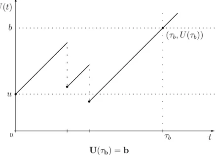
We denote this probability byξ(u, b), and letχ(u, b) denote the probability that the surplus process attains the levelbfrom initial surplusuwithout first falling below zero. To find expressions for ξ(u, b) and χ(u, b), we consider the ruin and survival probabilities respectively in an unrestricted surplus process. Let the random variable τb be the time to attain the level b, where

it is understood that τb =∞if the surplus never reachesb. This is shown in

Figure 2.4.

If survivals occurs from initial surplus u, then the surplus process must pass through the levelb > uat some point in time, as the net profit condition (2.3.1) implies thatU(t)→ ∞ast→ ∞with probability one (almost surely).

✲ ✻

U(t)

u b

U(τb) =b

♣ ♣ ♣ ♣ ♣ ♣ ♣ ♣ ♣ ♣ ♣ ♣ ♣ ♣ ♣ ♣ ♣ ♣ ♣ ♣ ♣ ♣ ♣ ♣ ♣ ♣ ♣ ♣ ♣ ♣ ♣ ♣ ♣ ♣ ♣ ♣ ♣ ♣ ♣ ♣ ♣ ♣ ♣ ♣ ♣ ♣ ♣ ♣ ♣ ♣ ♣ ♣ ♣ ♣ ♣ ♣ ♣ ♣ ♣ ♣ ♣ ♣ ♣ ♣ ♣ ♣ ♣ ♣ ♣ ♣ ♣ ♣ ♣ ♣ ♣ ♣ ♣ ♣ ♣ ♣ ♣ ♣ ♣ ♣ ♣ ♣ ♣ ♣ ♣ ♣ ♣ ♣ ♣ ♣ ♣ ♣ ♣ ♣ ♣ ♣ ♣ ♣ ♣ ♣ ♣ ♣ ♣ ♣

r r

r

(τb, U(τb))

♣ ♣ ♣ ♣ ♣ ♣ ♣ ♣ ♣ ♣ ♣ ♣ ♣ ♣ ♣ ♣ ♣

τb

0 _t

(35)

In the classical risk model, as the distribution of the time to the next claim from the time the surplus attainsb is exponential, the probabilistic behavior of the surplus process once it attains level b is independent of its behavior prior to attainingb. Hence Φ(u) =χ(u, b)Φ(b) or equivalently,

χ(u, b) = 1−Ψ(u) 1−Ψ(b).

Similarly, if ruin occurs from initial surplusu, then either the surplus process does or does not attain levelb prior to ruin. Hence

Ψ(u) =ξ(u, b) +χ(u, b)Ψ(b),

so that

ξ(u, b) = Ψ(u)− 1−Ψ(u)

1−Ψ(b)Ψ(b) =

Ψ(u)−Ψ(b) 1−Ψ(b) .

The reason for this is the memoryless property of the exponential distribu-tion.

In a Sparre–Andersen risk model, we no longer have that memoryless property, so the approach to find ξ(u, b) and χ(u, b) is different.

Considering the amount and the time of arrival of the first claim, we get renewal equations for χ(u, b) and ξ(u, b) that resemble those we had before for Φ(u) and Ψ(u)

χ(u, b) =

Z b−u

c

0

k(t)

Z u+ct

0

p(x)χ(u+ct−x, b)dxdt+

Z ∞

b−u

c

k(t)dt, (2.4.1)

and

ξ(u, b) =

Z b−u

c

0

k(t)

Z u+ct

0

p(x)ξ(u+ct−x, b)dx

+

Z ∞

u+ct

p(x)dx

dt. (2.4.2)

Then it is clear that

lim

b→∞χ(u, b) = Φ(u), and blim→∞ξ(u, b) = Ψ(u).

(36)

level b.

In the following chapters we present computations ofχ(u, b) by solving an integro–differential equation that it satisfies, which in turn depends on the nature of k(t).

2.4.2 The severity of ruin and its maximum

In this section we are interested not just in the probability of ruin, but also in the amount of the insurer’s deficit at the time of ruin, if ruin occurs.

Given an initial surplus u, recall that we denoted the time to ruin from initial surplus u byTu. Define

G(u, y) =P r(Tu <∞andU(Tu)≥ −y),

to be the probability that ruin occurs and that the insurer’s deficit at ruin, or severity of ruin, is at most y. We notice that

lim

y→∞G(u, y) = Ψ(u),

so that

G(u, y)

Ψ(u) =P r(|U(Tu)| ≤y)|Tu <∞)

is proper distribution function. Hence for a given initial surplusu, G(u, .) is a defective distribution with (defective) density

g(u, y) = ∂

∂yG(u, y).

We now allow surplus process to continue if ruin occurs, and we consider the insurer’s maximum severity of ruin from the time of ruin until the time that the surplus process next attains level 0. As we are assuming the net profit condition (2.3.1), it is certain that the surplus process will attain this level.

We define T′

u to be the time of the first upcrossing of the surplus process

through level 0 after ruin occurs and define the random variable Mu by

Mu = sup{|U(t)|, Tu ≤t≤Tu′},

so that Mu denotes the maximum severity of ruin. This is shown in Figure

2.5. Let

(37)

✲ ✻

U(t)

u

z

U(Tu)<0

U(T′

u) =0

♣ ♣ ♣ ♣ ♣ ♣ ♣ ♣ ♣ ♣ ♣ ♣ ♣ ♣ ♣ ♣ ♣ ♣ ♣ ♣ ♣ ♣ ♣ ♣ ♣ ♣ ♣ ♣ ♣ ♣ ♣ ♣ ♣ ♣ ♣ ♣ ♣ ♣ ♣ ♣ ♣ ♣ ♣ ♣ ♣ ♣ ♣ ♣ ♣ ♣ ♣ ♣ ♣ ♣

r r

r

T′

u

Tu

0 _t

❄ ✻

Mu

Figure 2.5: The maximum severity of ruin

to be the distribution function ofMu given that ruin occurs. The maximum

severity of ruin is no more than z if ruin occurs with a deficit y ≤ z and if the surplus does not fall below−z from the level −y. The probability of this latter event isχ(z−y, z) since attaining level 0 form level−y without falling below −z is equivalent to attaining level z from level z−y without falling below 0.

Then

J(z;u) =

Z z

0

g(u, y)

Ψ(u) χ(z−y, z)dy. (2.4.3) In the classical risk model we have Φ(u) = χ(u, b)Φ(b) and therefore we evaluate (2.4.3) by nothing that

Ψ(u+z) =

Z ∞

z

g(u, y)dy+

Z z

0

g(u, y)Ψ(z−y)dy. (2.4.4)

This follows by noting that if ruin occurs from initial surplus u+z, then the surplus process must fall below z at some time in the future.

(38)

Noting that Ψ = 1−Φ we can write equation (2.4.4) as

Z z

0

g(u, y)Φ(z−y)dy =

Z ∞

z

g(u, y)dy+

Z z

0

g(u, y)dy−Ψ(u+z)

= Ψ(u)−Ψ(u+z).

Thus,

J(z;u) = Ψ(u)−Ψ(u+z) Ψ(u)(1−Ψ(z))

However, this method can not be performed in the same way in the Sparre– Andersen model since, once again, we used the memoryless property in the process.

In the Sparre–Andersen model we work on a method to find J(z;u) in (2.4.3) that involves finding first the probability of attaining an upper barrier level χ(u, b).

2.4.3 The distribution of the time to ruin

Recall the random variable Tu denoting the time of ruin. The distribution

of Tu is important since P r(Tu ≤t) gives the probability that ruin occurs at

or before time t. If we know the distribution of Tu we are able to compute

finite time ruin probabilities. Define a function ϕ as

ϕ(u, δ) =E[e−δTu_I₍_T

u <∞)]

where δ is a non-negative parameter which we consider in this section as the parameter of a Laplace transform, and I _{is the indicator function, so that} I₍_A_{) = 1 if the event} _A _{occurs and equals 0 otherwise. Notice that}

lim

δ→0ϕ(u, δ) = E[

I₍_T_u _<_∞_{)] =} _{P r}_[_T_u _<_∞_{] = Ψ(}_u₎_.

In the next section of the expected discounted dividends we consider a function similar to ϕ, and in that function the interpretation of δ is that it is a force of interest. With this interpretation, ϕ(u, δ) gives the expected present value of 1 payable at the time of ruin.

(39)

In the classical risk model we have

ϕ(u, δ) =

Z ∞

0

λe−λte−δt

Z u+ct

0

p(x)ϕ(u+ct−x, δ)dxdt

+

Z ∞

0

λe−λte−δt

Z ∞

u+ct

p(x)dxdt. (2.4.5)

Substitutings=u+ctin equation (2.4.5) gives

ϕ(u, δ) = λ

c

Z ∞

u

e−(λ+δ)(s−u)/c

Z s

0

p(x)ϕ(s−x, δ)dxds

+ λ

c

Z ∞

u

Z ∞

s

p(x)dxds.

Afterwards, we differentiate this equation with respect to u to obtain an integro–differential equation

∂

∂uϕ(u, δ) = λ+δ

c ϕ(u, δ)− λ

c

Z u

0

p(u−x)ϕ(x, δ)dx− λ

c(1−P(u)).

In the Sparre–Andersen risk model the renewal equation is given by

ϕ(u, δ) =

Z ∞

0

k(t)e−δt

Z u+ct

0

p(x)ϕ(u+ct−x, δ)dxdt

+

Z ∞

0

k(t)e−δt

Z ∞

u+ct

p(x)dxdt. (2.4.6)

Any further developments will depend on the specific characteristics of the density ofk(t).

2.5 Expected discounted dividends

We now consider a problem where an insurance portfolio is used to provide dividend income for the insurance company’s shareholders. Specifically, let

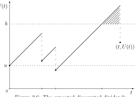
udenote the initial surplus and let b ≥ube a dividend barrier.

Whenever the surplus attains the level b, the premium income is paid to shareholders as dividends until the next claim occurs, so that in this modified surplus process, the surplus never attains a level greater than b, see Figure 2.6.

(40)

✲ ✻

U(t)

u b ♣ ♣ ♣ ♣ ♣ ♣ ♣ ♣ ♣ ♣ ♣ ♣ ♣ ♣ ♣ ♣ ♣ ♣ ♣ ♣ ♣ ♣ ♣ ♣ ♣ ♣ ♣ ♣ ♣ ♣ ♣ ♣ ♣ ♣ ♣ ♣ ♣ ♣ ♣ ♣ ♣ ♣ ♣ ♣ ♣ ♣ ♣ ♣ ♣ ♣ ♣ ♣ ♣ ♣ ♣ ♣ ♣ ♣ ♣ ♣ ♣ ♣ ♣ ♣ ♣ ♣ ♣ ♣ ♣ ♣ ♣ ♣ ♣ ♣ ♣ ♣ ♣ ♣ ♣ ♣ ♣ ♣ ♣ ♣ ♣ ♣ ♣ ♣ ♣ ♣ ♣ ♣ ♣ ♣ ♣ ♣ ♣ ♣ ♣ ♣ ♣ ♣ ♣ ♣ ♣ ♣ ♣ ♣♣ ♣♣ ♣♣ ♣♣ ♣♣ ♣♣ ♣♣ ♣♣ ♣♣ ♣♣ ♣♣ ♣♣ ♣♣ ♣♣ ♣♣ ♣♣ ♣♣ ♣♣ ♣ ♣♣ ♣♣ ♣♣ ♣♣ ♣♣ ♣♣ ♣♣ ♣♣ ♣♣ ♣♣ ♣♣ ♣♣ ♣♣ ♣♣ ♣ ♣ ♣♣ ♣♣ ♣♣ ♣♣ ♣♣ ♣♣ ♣♣ ♣♣ ♣♣ ♣♣ ♣♣ ♣♣ ♣ ♣♣ ♣♣ ♣♣ ♣♣ ♣♣ ♣♣ ♣♣ ♣♣ ♣♣ ♣ ♣ ♣♣ ♣♣ ♣♣ ♣♣ ♣♣ ♣♣ ♣♣ ♣ ♣♣ ♣♣ ♣♣ ♣♣ ♣ ♣ ♣♣ ♣♣ r r r r (t, U(t))

0 _t

Figure 2.6: The expected discounted dividends

for the modified surplus process. We represent the modified surplus process in Figure 2.7.

Let us assume that the shareholders provide the initial surplus uand pay the deficit at ruin. An interesting question is how the level of the barrier b

should be chosen to maximize the expected present value of net income to the shareholders, assuming that there is no further business after the time of ruin. Another interesting question is how the situation changes when we introduce capital injections after the time of ruin.

We define V(u, b) to be the expected present value at force of interest δ

of dividends payable to shareholders prior to ruin, Yu,b to be the deficit at

ruin andTu,b to be the time of ruin, so thatE[Yu,b e−δTu,b] gives the expected

present value of the deficit at ruin. Then we want to choose b such that the following function

L(u, b) = V(u, b)−E[Yu,b e−δTu,b]−u

is maximized, and to address this question we must consider the components of L(u, b).

We can find an expression for V(u, b) by the standard technique of con-ditioning on the time and the amount of the first claim. We note that for

(41)

✲ ✻

U(t)

u b

♣ ♣ ♣ ♣ ♣ ♣ ♣ ♣ ♣ ♣ ♣ ♣ ♣ ♣ ♣ ♣ ♣ ♣ ♣ ♣ ♣ ♣ ♣ ♣ ♣ ♣ ♣ ♣ ♣ ♣ ♣ ♣ ♣ ♣ ♣ ♣ ♣ ♣ ♣ ♣ ♣ ♣ ♣ ♣ ♣ ♣ ♣ ♣ ♣ ♣ ♣ ♣ ♣ ♣ ♣ ♣ ♣ ♣ ♣ ♣ ♣ ♣ ♣ ♣ ♣ ♣ ♣ ♣ ♣ ♣ ♣ ♣ ♣ ♣ ♣ ♣ ♣ ♣ ♣ ♣ ♣ ♣ ♣ ♣ ♣ ♣ ♣ ♣ ♣ ♣ ♣ ♣ ♣ ♣ ♣ ♣ ♣ ♣ ♣ ♣ ♣ ♣ ♣ ♣ ♣ ♣ ♣ ♣

r r

r

r (t, U(t))

0 _t

Figure 2.7: The modified surplus

In the classical risk model, for 0≤u < b, the renewal equation is

V(u, b) = e−(λ+δ)τV(b, b) +

Z τ

0

λe−(λ+δ)t

Z u+ct

0

p(x)V(u+ct−x, b)dxdt.

Substitutings=u+ctwe obtain

V(u, b) = e−(λ+δ)(b−u)/c_V₍_{b, b}₎

+λ

c

Z b

u

Z s

0

p(x)V(s−x, b)dxds,

and differentiating with respect to uwe get

∂

∂uV(u, b) = λ+δ

c V(u, b)− λ

c

Z u

0

p(x)V(u−x, b)dxdt. (2.5.1)

Similarly, by considering dividends payments before and after the first claim, we have

V(b, b) =

Z ∞

0

λe−(λ+δ)tcstdt

+

Z ∞

0

λe−(λ+δ)t

Z b

0

p(x)V(b−x, b)dxdt, (2.5.2)

wheres_t = (eδt₋₁₎_/δ_{is the accumulated amount at time}_t_{at force of interest}

(42)

Integrating out in equation (2.5.2) we obtain

V(b, b) = c

λ+δ + λ λ+δ

Z b

0

p(x)V(b−x, b)dx. (2.5.3)

From equation (2.5.1) we find that

c λ+δ

∂

∂uV(u, b)

u=b

=V(b, b)− λ

λ+δ

Z b

0

p(x)V(b−x, b)dx,

which, together with equation (2.5.3), gives the boundary condition

∂

∂uV(u, b)

u=b

= 1.

In the Sparre–Andersen risk model the renewal equation for V(u, b) takes the form

V(u, b) =

Z ∞

b−u

c

k(t)e−δt

c s_t₋b−u

c

+

Z b

0

p(x)V(b−x, b)dx

dt+

+

Z b−u

c

0

e−δtk(t)

Z u+ct

0

V(u+ct−x, b)p(x)dx dt. (2.5.4)

Furthermore, let the random variable Du,b denote the present value at force

of interest δ(> 0) per unit time of dividends payable to shareholders until ruin occurs, and denote m–th moment as Vm(u, b) =E[Dmu,b], m≥ 0, where

V0(u, b)≡1. Then we haveV1(u, b) =V(u, b).

A renewal equation forVm(u, b), m ≥1 is the following

Vm(u, b) =

Z ∞

b−u

c

k(t)e−mδt

c s

t−b−u

c m + + m X j=1 m

j c st−b−u

c

m−jZ b

0

p(x)V_j(b−x, b)dx

  dt+

+ Z b−u

c

0

e−mδtk(t) Z u+ct

0

Vm(u+ct−x, b)p(x)dx dt. (2.5.5)

(43)

2.6 Final remarks

(44)

Chapter 3 The Sparre–Andersen model

with Erlang(

n

) interclaim times

The only way to learn mathematics is to do mathematics

Paul Halmos

3.1 Introduction

In this chapter we study the Sparre–Andersen risk model under the assump-tion that the interclaim times are Erlang(n) distributed.

In Section 3.2 we investigate the fundamental and the generalized Lund-berg’s equations, take a closer look at the roots of these equations and assume the net profit condition. The most important result of this section say that the roots of the equations mentioned above are distinct.

In Section 3.3 we present results from Li and Dickson (2006) and Li (2008b) which are part of the mathematical foundation for the chapter. In particular we begin by describing the problem of finding the survival proba-bility and the probaproba-bility of attaining an upper barrier prior to ruin.

A new theorem for obtaining the latter is given in section 3.4.

We continue in Section 3.5 applying our theorem for the maximum severity of ruin.

(45)

In the last section of this chapter we focus on dividends, where numerical examples are provided.

3.2 The Lundberg’s equation

The density of the interclaim time Wi, which we denote as kn(t),

kn(t) =

λn_tn−1_e−λt

(n−1)! , t ≥0, λ >0, n∈N

+_,

and its probability distribution function denoted as

Kn(t) = 1− n−1

X

i=0

(λt)i_e−λt

i! .

The most important properties of this distribution are the following

ˆ

kn(s) =

λ λ+s

n

,

k′_n(t) = λ(kn−1(t)−kn(t)),

k_n(i)(0) = 0, i= 0, . . . , n−2, k(_nn−1)(0) = λn,

which we use later on this chapter.

The fundamental Lundberg’s equation from the previous chapter (2.3.4) can be written in the form

λ c −s

n

=

λ c

n

ˆ

p(s). (3.2.1)

On the other hand we have the generalized Lundberg’s equation (2.3.5)

ex-pressed as

λ+δ c −s

n

=

λ c

n

ˆ

p(s), (3.2.2)

whereδ >0 is the force of interest. We consider this equation in the section of dividends.

(46)

are different. We can find in Ji and Zhang (2011) a detailed explanation of this result. By the numbers ρ1, ρ2, . . . , ρn−1 ∈ C denote the roots of (3.2.1)

which have positive real parts, and R >0 is the adjustment coefficient. We assume the net profit condition (2.3.1), which in our case becomes

cE[Wi]> E[Xi]⇐⇒c

n

λ > µ1. (3.2.3)

3.3 Mathematical background

In the literature of risk theory, it is common to work with integro–differential equations.

We know from Li and Dickson (2006) that the probability of attaining an upper barrier prior to ruin, χ(u, b), satisfies an order n integro–differential equation with n boundary conditions. This can be written in the form

B(D)v(u) =

Z u

0

v(u−y)p(y)dy, u≥0, (3.3.1)

where

B(D) =I −c

λ

Dn =

n

X

k=0

(−1)kc

λ

k_n

k

Dk =

n

X

k=0

BkDk,

and Bk = (−1)k _λc

k _n k

.

The operator D = d/du denotes differentiation with respect to u and I

is the identity operator. Thus, B(D) is a differential operator of degree n. If we find n linearly independent particular solutions vj(u), j = 1, . . . , n for

this equation, then we have

χ(u, b) =−→v(u)[V(b)]−1−→eT, (3.3.2) where −→v(u) = (v1(u), . . . , vn(u)) is a 1×n vector, V(b) is a n ×n matrix

with entries given by

(V(b))ij =

di−1_v

j(u)

dui−1

u=b

and −→e = (1,0, . . . ,0) which is a 1× n vector. We can find a complete derivation of this result in Li (2008a).

(47)

In this chapter our aim is to seek for those solutions, which in turn depend on the roots of the fundamental Lundberg’s equation. Li (2008a) finds a vector of solutions −→v (u) for the case when ρ1, ρ2, . . . , ρn−1 are all distinct.

Our work starts by giving an improved version for the expressions pre-sented by Li (2008a) for the functions vi(u), i = 1, . . . , n. This is given in

the next section. Further, we apply our results in order to find the distribu-tion of the maximum severity of ruin.

Afterwards, we deal with the dividends problem, we mean the calculation of the moments Vm(u, b). As we mentioned before for a classical risk model,

an integro–differential equation for V(u, b) can be found in Dickson (2005), and for Vm(u, b) in Dickson and Waters (2004). For the Erlang(n) model

we give the respective integro–differential equations as well as a method of finding the solutions of this equations.

3.4 Solutions

for

the

integro-differential

equation

In this part we consider the relation between the roots of the fundamental Lundberg’s equation that have positive real parts and the solutions for the integro-differential equation ((3.3.1)). Li (2008a) found that

Theorem 3.4.1 If ρ1, ρ2, . . . , ρn−1 ∈ C are distinct, then we have the

fol-lowing expressions for thevj(u)’s

v1(u) = Φ(u), vj(u) =

j−1

X

i=1 ai,j

Z u

0

Φ(u−y)eρiy_dy, _j _{= 2}_,₃_{, . . . , n,}

where ai,j =−

1

Qj−1

k=1,k6=i(ρk−ρi)

, i= 1,2, . . . , j−1.

We introduce developments, proposing a new version of Theorem 3.4.1:

Theorem 3.4.2 If ρ1, ρ2, . . . , ρn−1 ∈ C are distinct, then we have the

fol-lowing expressions for thevj(u)’s

v1(u) = Φ(u), vj(u) =

Z u

0

(48)

Proof: Any solution v(u) of (3.3.1) has Laplace transform

ˆ

v(s) = dv(s)

B(s)−pˆ(s),

where

dv(s) = n−1

X

i=0

n

X

k=i+1

n k

−c λ

k

v(k−1−i)(0)

!

si

=

n−1

X

i=0

n

X

k=i+1

Bkv(k−1−i)(0)

!

si.

The survival probability Φ(u) is a solution of (3.3.1), and its Laplace trans-form is given by [see Li (2008a)]

ˆ

Φ(s) = −Φ(0)c

λ

nQn−1

i=1(ρi−s) B(s)−pˆ(s) ,

we denote

dΦ(s) =−Φ(0)

_c

λ

nnY−1 i=1

(ρi−s). (3.4.1)

Now we show that any function vj(u) =

Ru

0 Φ(u − y)e

ρj−1ydy, with j = 2,3, . . . , n,is solution of (3.3.1). We need to prove that

B(D)vj(u) = dΦ(ρj−1)eρj−1u+

Z u

0

(B(D)Φ(u−t))eρj−1tdt

and that _Z _u

0

vj(u−y)p(y)dy=

Z u

0

(B(D)Φ(u−t))eρj−1tdt.

For the left hand side, the k-th derivative of vj(u) gives

v_j(k)(u) =

k−1

X

i=0

Φ(k−1−i)₍₀₎_ρi j−1

!

eρj−1u+

Z u

0

(49)

Therefore,

B(D)vj(u) = n

X

k=0

Bkv(jk)(u) =

=

n

X

k=0

Bk k−1 X

i=0

Φ(k−1−i)(0)ρi_j₋₁

!

eρj−1u+

n X k=0 Bk Z u 0

Φ(k)(u−y)eρj−1ydy

=

n−1 X

i=0

n

X

k=i+1

BkΦ(k−1−i)(0)

!

ρi_j₋₁

!

eρj−1u+

Z u

0

n

X

k=0

BkΦ(k)(u−y)

!

eρj−1ydy

= dΦ(ρj−1)eρj−1u+

Z u

0

n

X

k=0

BkΦ(k)(u−y)

!

eρj−1ydy

= Z u

0

(B(D)Φ(u−y))eρj−1ydy,

since dΦ(ρj−1) = 0, j = 2, . . . n from (3.4.1).

And for the right hand side we get

Z u

0

vj(u−x)p(x)dx =

Z u

0

Z u−x

0

Φ(u−x−y)eρj−1ydy

p(x)dx

=

Z u

0

Z u−y

0

Φ(u−y−x)p(x)dx

eρj−1ydy

=

Z u

0

(B(D)Φ(u−y))eρj−1ydy.

We have just proved that the functionsvj(u) are solutions of (3.3.1).

The only remaining part to prove is that those vj(u)’s are linearly

inde-pendent. We do this in the following way.

Suppose that we have a linear combination such that Pn_j₌₁cjvj(u) = 0,

(50)

(i) For c1 = 0. Let H(t) =P_jn₌₂cjeρj−1t, then

n

X

j=1

cjvj(u) = n

X

j=2 cj

Z u

0

Φ(u−y)eρj−1ydy

=

Z u

0

Φ(u−y)

n

X

j=2

cjeρj−1ydy

= Φ∗H(u) = 0.

The fact that Φ∗H(u) = 0,∀u≥0 with Φ(u)6≡0, implies thatH(u)≡

0 almost everywhere. But on the other side H(t) is a continuously differentiable function, this implies that c1 =c2 =· · ·=cn= 0.

(ii) For c1 6= 0. We define G(t) = Pn_j₌₂(−cj/c1)eρj−1t, so Φ ∗G(u) =

Φ(u)∀u≥0. Not all the remaining coefficients cj’s can be 0, otherwise

G(t) ≡ 0. But then limu→+∞G(u) = ±∞ depending on the sign of

the non zero coefficients. As Φ(u) is a non–decreasing non–negative function with limu→+∞Φ(u) = 1, we have that limu→+∞Φ∗G(u) =

±∞, which is a contradiction and concludes the proof.

Remark 3.4.1 For any complex rootρof the fundamental Lundberg’s equa-tion the conjugate ¯ρis also a root, we have thatv(u) = R₀uΦ(u−y)eρy_dy_and

its conjugate v(u) =R₀uΦ(u−y)eρy¯ _dy_{are both solutions of (3.3.1). We take}

advantage of this fact in Theorem 3.4.2. Thus, for computational purposes this theorem becomes much simpler than Theorem 3.4.1.

3.5 The maximum severity of ruin

In the previous section we have shown how to obtain the solutions of the integro–differential equation. Now, we use these results to obtain the corre-sponding expressions for the distribution of the maximum severity of ruin. We find an expression for that distribution which only depends on the non-ruin probability Φ(u) and the claim amounts distribution.

From Dickson (2005) and (3.3.2) we know that the distribution of the maximum severity of ruin J(z;u) can be expressed as:

J(z;u) = 1 1−Φ(u)

Z z

0

(51)

For simplicity we denote by

− →

h(z, u) =

Z z

0

g(u, y)(v1(z−y), . . . , vn(z−y))dy

=

Z z

0

g(u, y)v1(z−y)dy, . . . ,

Z z

0

g(u, y)vn(z−y)dy

= (h1(z, u), . . . , hn(z, u)),

In this moment the only remaining part to find is an expression for every component of −→h(z, u). We consider the case of the Theorem 3.4.2 like in the previous section. In a similar way as it is done by Li (2008a) we get for

j = 1: _Z

z

0

g(u, y)v1(z−y)dy= Φ(u+z)−Φ(u), (3.5.2)

and for j = 2, . . . , n:

Z z

0

g(u, y)vj(z−y)dy =

Z z

0

g(u, y)

Z z−y

0

Φ(z−y−x)eρj−1xdxdy

=

Z z

0

eρj−1x[Φ(u+ (z−x))−Φ(u)]dx.

Hence we get the desired expression for the maximum severity of ruin.

3.6 Explicit expressions

In this section our aim is to determine explicit expressions for the (existing) moments of the maximum severity of ruin as well as the probability that the maximum severity occurs at ruin. Li (2008a) considered those moments for Erlang(2) interclaim times and exponential claims. We work here with other two cases and present formulae as well as some numerical calculations. Namely, for cases where:

1. Interclaim arrivals are Erlang(3,λ) and single claim amounts are exponential(β) distributed. For simplification we denote this case by Erlang(3)–exponential;

INSTITUTO SUPERIOR DE ECONOMIA E GEST ˜

UNIVERSIDADE DE LISBOA