Full Terms & Conditions of access and use can be found at
http://www.tandfonline.com/action/journalInformation?journalCode=sact20
Download by: [b-on: Biblioteca do conhecimento online UTL] Date: 13 October 2015, At: 08:33
Scandinavian Actuarial Journal
ISSN: 0346-1238 (Print) 1651-2030 (Online) Journal homepage: http://www.tandfonline.com/loi/sact20
Further developments in the Erlang(n) risk process
Agnieszka I. Bergel & Alfredo D. Egídio Dos Reis
To cite this article: Agnieszka I. Bergel & Alfredo D. Egídio Dos Reis (2015) Further
developments in the Erlang(n) risk process, Scandinavian Actuarial Journal, 2015:1, 32-48, DOI: 10.1080/03461238.2013.774112
To link to this article: http://dx.doi.org/10.1080/03461238.2013.774112
Published online: 31 May 2013.
Submit your article to this journal
Article views: 139
View related articles
Vol. 2015, No. 1, 32–48, http://dx.doi.org/10.1080/03461238.2013.774112
Further developments in the Erlang(
n
) risk process
AGNIESZKA I. BERGEL and ALFREDO D. EGÍDIO DOS REIS∗
Department of Mathematics, ISEG and CEMAPRE, Technical University of Lisbon, Lisbon, Portugal
(Accepted 3 February 2013)
For actuarial aplications, we consider the Sparre–Andersen risk model when the interclaim times are Erlang(n) distributed. We first address the problem of solving an integro-differential equation that is satisfied by the survival probability and other probabilities, and show an alternative and improved method to solve such equations to that presented by Li (2008).
This is done by considering the roots with positive real parts of the generalized Lundberg’s equation, and establishing a one–one relation between them and the solutions of the integro-differential equation mentioned before.
Afterwards, we apply our findings above in the computation of the distribution of the maximum severity of ruin. This computation depends on the non-ruin probability and on the roots of the fundamental Lundberg’s equation.
We illustrate and give explicit formulae for Erlang(3) interclaim arrivals with exponentially distributed single claim amounts and Erlang(2) interclaim times with Erlang(2) claim amounts.
Finally, considering an interest force, we consider the problem of calculating the expected discounted dividends prior to ruin, finding an integro-differential equation that they satisfy and solving it. Numerical examples are also provided for illustration.
Keywords: Sparre–Andersen risk model; Erlang(n) interclaim times; fundamental Lundberg’s equation; gen-eralized Lundberg’s equation; probability of reaching an upper barrier; maximum severity of ruin; expected discounted dividends prior to ruin
1. Introduction
In the present article, we work with the Sparre–Andersen model driven by the equation
U(t)=u+ct− N(t)
i=1
Xi, t≥0,
whereu(≥0) is the initial capital,c(≥0) is the premium income per unit timet,{Xi}∞i=1 is a sequence of (i.i.d.) independent and identically distributed random variables, each representing a single claim amount, with common distribution functionP(x)and density p(x). Its Laplace transform is denoted bypˆ(.). Denote byµk = E[X1k]thek-th moment of Xi. We assume the
existence ofµ1(this is a general condition and it is crucial for setting the positive loading factor
∗Corresponding author. E-mail: [email protected]
© 2013 Taylor & Francis
assumption below). In some parts of this manuscript, we will work with cases where higher moments exist. The sequence{Xi}is independent of the counting process{N(t),t≥0}, with N(t)=max{k:W1+W2+ · · · +Wk≤t}where the random variablesWi,i ∈N+, are i.i.d.
and Erlang(n,λ) distributed, with densitykn(t),
kn(t)=
λntn−1e−λt
(n−1)! , t≥0, λ >0,n∈N +
and probability distribution function
Kn(t)=1− n−1
i=0
(λt)ie−λt i! .
We assume a positive loading factor, that isc E(W1) >E(X1)⇔cn> λµ1.
Moreover, the adjustment coefficientR>0 is the smallest positive number such that−Ris a solution of the Lundberg equation
1−c
λ
sn = ˆp(s).
Now, we set some definitions and mathematical preliminaries regarding on main objects of interest in the Sparre–Andersen model. Time to ruin is denoted asT =inf{t >0 : U(t) < 0|U(0)=u}, andT = ∞ if and only if U(t)≥0, ∀t >0. The ultimate ruin probability is defined as(u)=Pr(T <∞)and the corresponding non-ruin probability is(u)=1−(u). Regarding the barrier problem, which is related to the payment of dividends, we denote by τb=inf{t >0:U(t)≥b|U(0)=u}the first time that the surplus upcrosses the levelb≥u.
The probability that the surplus attains the levelbfrom initial surplusu without first falling below zero is given by
χ (u,b)=Pr(T > τb|U(0)=u),
withξ(u,b)=1−χ (u,b)being the probability that ruin occurs fromubefore the surplus ever reachingb.
Assuming that the surplus process continues after ruin, we denote the time of the first upcross of the surplus through level ‘0’ after ruin occurs byT′=inf{t: t>T, U(t)≥0}, for finite T. In the interval of time where the surplus is at deficit, we define the maximum severity of ruin as
Mu=sup{|U(t)| : T ≤t≤T′|U(0)=u}.
The conditional distribution function of the maximum severity of ruin, given that ruin occurs, is given by
J(z;u)=Pr(Mu≤z|T <∞), u,z≥0.
The probability that ruin occurs and that the deficit at ruin is at mostyis given byG(u,y)= P(T < ∞,U(T) ≥ −y|U(0) =u). For a givenu, this is a defective distribution function, clearly limy→∞G(u,y)=(u). The corresponding (defective) density is denoted asg(u,y).
The probability that the maximum deficit occurs at ruin is defined by Pr(Mu= |U(T)| |T <∞).Picard(1994) showed that
P(Mu= |U(T)| |T <∞)= ∞
0 g(u,y)χ (0,y)d y
(u) . (1.1)
We consider the problem where an insurance portfolio is used to provide dividend income for that insurance’s company shareholders. Like before, letudenote the initial surplus and let b≥ube a dividend barrier. Let the random variableDudenote, the present value at a positive
constant force of interest per unit time of dividends payable to shareholders until ruin occurs, and denotem-th moment asVm(u,b)= E[Dum], m ≥0, whereV0(u,b) ≡1. For simplicity
we will denoteV1(u,b)=V(u,b). We assume the existence ofVm(u,b).
In the next section, we present some of the mathematical background on the model related to our problem. In Sections 3 and 4, we study the integro-differential equation and show explicit formulas for the maximum severity of ruin. Section 5 is devoted to some particular cases where explicit expressions can easily be found. In Section 6, we give attention to the dividends problem. Finally, in the last section we state some concluding remarks.
2. Mathematical background
In recent years, the Sparre–Andersen model has been a major point of interest in risk theory. Many authors have done a lot of important advances in the topic. In this paper, we present some new developments.
We know from Li & Dickson (2006) that χ (u,b) satisfies an ordern integro-differential equation withnboundary conditions that can be written in the form
B(D)v(u)= u
0
v(u−y)p(y)d y, u≥0, (2.1)
where
B(D)=I−c
λ
D
n =
n
k=0
(−1)kc λ
k
n k
Dk,
andD is the differential operator. See alsoLi(2008). If we findnlinearly independent particular solutionsvj(u), j=1, . . . ,nfor this equation, then we have
χ (u,b)= −→v (u)[V(b)]−1−→e′, (2.2)
where−→v (u)=(v1(u), . . . , vn(u))is a 1×nvector,V(b)is an×nmatrix with entry given by
(V(b))i j = di−1v
j(u) dui−1
u=b
and−→e =(1,0, . . . ,0)is a 1×nvector.
In this manuscript, we will be seeking for those solutions, which in turn depend on the roots of the fundamental Lundberg’s equation. Recall that the fundamental Lundberg’s equation is given by
λ
c −s n
=
λ
c n
ˆ
p(s). (2.3)
We denote by the numbersρ1, ρ2, . . . , ρn−1 ∈ C, the roots of this equation which have
positive real parts (there are of course other roots, among them is 0 and−R, whereR>0 is the adjustment coefficient, seeLi & Garrido(2004)).
On the other hand, the generalized Lundberg’s equation is given by
λ+δ
c −s n
=
λ
c n
ˆ
p(s), (2.4)
whereδis a positive constant force of interest. This equation has exactlynroots with positive real parts and will be considered in the section of dividends. SeeLi & Garrido(2004).
Li(2008) finds the vector of solutions−→v (u)for the case whenρ1, ρ2, . . . , ρn−1are all distinct
(in fact, all those roots are different, according toJi & Zhang(2011)).
Our work start, by giving an improved version for the expressions given byLi(2008) for thevi(u), i = 1, . . . ,n. This will be given in the next section. Then, we apply our results
in order to find the corresponding expressions for the distribution of the maximum severity of ruin. Afterwards, we deal with the dividends problem, we mean the calculation of the moments Vm(u,b). For a Poisson model, an integro-differential equation for V(u,b)can be found in Dickson(2005), and forVm(u,b)inDavidet al.(2004). For the Erlang(n) model, we give the
respective integro-differential equations as well as a method to find their solutions.
3. Solutions for the integro-differential equation
Let us consider the relation between the roots of the fundamental Lundberg’s equation that have positive real parts and the solutions for the integro-differential Equation (2.1).Li(2008) found that
Th e o r e m 3.1 Ifρ1, ρ2, . . . , ρn−1∈Care distinct, then we have the following expressions for
thevj(u)’s
v1(u) = (u),
vj(u) = j−1
i=1 ai,j
u 0
(u−y)eρiyd y, j =2,3, . . . ,n,
where ai,j = −
1
j−1
k=1,k=i(ρk−ρi)
, i =1,2, . . . ,j−1.
Considering our developments, we propose instead a new version of Theorem3.1, as follows:
Th e o r e m 3.2 Ifρ1, ρ2, . . . , ρn−1∈Care distinct, then we have the following expressions for
thevj(u)’s
v1(u) = (u),
vj(u) = u
0
(u−y)eρj−1yd y, j =2,3, . . . ,n.
Proof We know fromLi(2008) that any solutionv(u)of (2.1) has Laplace transform
ˆ
v(s)= dv(s) B(s)− ˆp(s),
where
dv(s)= n−1
i=0 ⎛
⎝ n
k=i+1
n k
−c
λ
k
v(k−1−i)(0)
⎞
⎠si.
Since(u)is solution of (2.1), its Laplace transform is given by [seeLi(2008)]
ˆ
(s)= −(0)
c
λ
n n−1 i=1(ρi−s) B(s)− ˆp(s) ,
then we have
d(s)= −(0) c
λ
nn−1
i=1
(ρi−s).
Now, let us see that any functionvj(u) = u
0 (u− y)eρj−1yd y, with j = 2,3, . . . ,n,is
solution of (2.1). We can show that
B(D)vj(u)=d(ρj−1)eρj−1u+ u
0
(B(D)(u−t))eρj−1tdt
and that
u 0
vj(u−y)p(y)d y= u
0
(B(D)(u−t))eρj−1tdt.
Sinced(ρj−1)=0, j =2, . . .n,we get the desired equality. It remains to prove that those
vj(u)’s are linearly independent.
Suppose that we have a linear combination such thatnj=1cjvj(u)=0,∀u≥0. Consider
the cases (i) and (ii) below.
(i) c1=0:
LetH(t)=n
j=2cjeρj−1t, then n
j=1
cjvj(u) = n
j=2 cj
u 0
(u−y)eρj−1yd y
= u
0
(u−y)
n
j=2
cjeρj−1yd y
= ∗H(u)=0.
The fact that∗H(u)=0,∀u≥0 with(u)≡0, impliesH(u)≡0 almost everywhere. ButH(t)is a continuously differentiable function, this implies thatc1=c2= · · · =cn=0.
(ii) c1=0:
DefineG(t)=n j=2
−cj/c1
eρj−1t, so∗G(u)=(u), ∀u≥0. Not all the remaining
coefficientscj’s can be 0, otherwiseG(t)≡0. But then limu→+∞G(u)= ±∞depending
on the sign of the non zero coefficients. As(u)is a non-decreasing non-negative function with limu→+∞(u) = 1, we will have that limu→+∞∗G(u) = ±∞, which is a
contradiction.
This completes the proof.
One advantage of Theorem3.2, is that, since for any complex rootρ of the fundamental Lundberg’s equation the conjugateρ¯is also a root, we will have thatv(u)=u
0 (u−y)eρyd y
and its conjugatev(u)=u
0 (u−y)eρ¯yd yare both solutions of (2.1).
Although Theorems3.1and3.2are equivalent, for large values ofnit is better to use Theorem
3.2for computational purposes.
It is easy to prove that in Erlang(n) model we do not have possibility of multiple roots, following the argument provided byJi & Zhang(2011),
Th e o r e m 3.3 In the Sparre–Andersen risk model, with interclaim times Erlang(n) distributed,
the n roots with positive real parts of the generalized Lundberg’s Equation(2.4)are all distinct.
Proof SeeJi & Zhang(2011), page 3.
Co r o l l a r y 3.1 In the Sparre–Andersen risk model, with interclaim times Erlang(n)
dis-tributed, the n−1roots with positive real parts of the fundamental Lundberg’s Equation(2.3) are all distinct.
4. The maximum severity of ruin
In the previous section we showed how to obtain the solutions of the integro-differential equation. Now we will use these results to obtain corresponding expressions for the distribution of the maximum severity of ruin. We will find an expression for that distribution which only depends on the non-ruin probability(u)and the claim amounts distribution.
If we denote by
− →
h(z,u) = z
0
g(u,y)(v1(z−y), . . . , vn(z−y))d y
=
z
0
g(u,y)v1(z−y)d y, . . . , z
0
g(u,y)vn(z−y)d y
= (h1(z,u), . . . ,hn(z,u)),
Then fromDickson(2005) and (2.2) we know that the distribution of the maximum severity of ruinJ(z;u)can be expressed as:
J(z;u)= 1 1−(u)
z 0
g(u,y)(v1(z−y), . . . , vn(z−y))d y[V(z)]−1−→e ′, (4.1)
and we only have to find an expression for every component of−→h(z,u). Considering the case of the Theorem3.2in the previous section:
In a similar way as it is done byLi(2008) we get forj=1:
z 0
g(u,y)v1(z−y)d y=(u+z)−(u), (4.2)
and forj=2, . . . ,n:
z 0
g(u,y)vj(z−y)d y = z
0
g(u,y)
z−y 0
(z−y−x)eρj−1xd x d y
= z
0
eρj−1x[(u+(z−x))−(u)]d x.
5. Explicit expressions
In this section, our aim is to determine explicit expressions for the (existing) moments of the maximum severity of ruin as well as the probability that the maximum severity occurs at ruin, for some cases.Li(2008) considered those moments for Erlang(2) interclaim times and exponential claims. We work here other two cases, and will be presenting formulae as well as some numerical calculations. Namely, for cases where:
(1) Interclaim arrivals are Erlang(3,λ) and single claim amounts are Exponential(β) distributed. For simplification, we denote this case by Erlang(3)–Exponential; (2) Interclaim arrivals are Erlang(2,λ) and single claim amounts are Erlang(2,β)
dis-tributed. Similarly, we denote this case by Erlang(2)–Erlang(2).
5.1. Erlang(3) – Exponential case
Considering the premium per unit timec=(1+θ )λ/3βwith safety loading coefficientθ >0, the fundamental Lundberg’s Equation (2.3) takes the form
1−c
λ
s3− β
(s+β) =0,
which has four roots: 0, ρ1, ρ2 and −R, where 0< R < β is the adjustment coefficient,
ρ1, ρ2 are complex roots with positive real parts and ρ2 = ρ1. The three solutions for the
integro-differential Equation (2.1) come
(u) = 1−
1− R
β
e−Ru,
v2(u) = −1
ρ1
+ β−R
β(R+ρ1)
e−Ru+ R(β+ρ1)
ρ1β(R+ρ1) eρ1u,
v3(u) = −1
ρ2
+ β−R
β(R+ρ2)
e−Ru+ R(β+ρ2)
ρ2β(R+ρ2) eρ2u.
5.1.1. Distribution and moments of the maximum severity
After calculating (4.1), we get the distribution of the maximum severity of ruin
1−J(z;u)= αe −Rz
1−γe−(ρ1+R)z−δe−(ρ2+R)z−ηe−Rz,
where
α= R(R+ρ1)(R+ρ2)
β(β+ρ1)(β+ρ2)
;γ = − R(β−R)(R+ρ2)
ρ1(β+ρ1)(ρ2−ρ1) ;
δ= R(β−R)(R+ρ1)
ρ2(β+ρ2)(ρ2−ρ1)
;η= (β−R)(R+ρ1)(R+ρ2)
βρ1ρ2
,
with 0< α <1, δ=γ and 0< η=1−α−γ −δ. Since we work with exponential claim amounts, note that this expression is independent fromu. However, in practice, depending on the risk aversion of the insurer, the loading factor (and thereforeR) might depend on the initial wealthu.
Consider now the moments ofMu, given that ruin occurs, ther-th moment is given by the
formula
E(Mur|T<∞) = r
∞
0
zr−1(1−J(z;u))d z
= rα
∞
0
zr−1e−Rz
1−γe−(ρ1+R)z−δe−(ρ2+R)z−ηe−Rz d z, (5.1)
Table 5.1. Expected values and standard deviations ofMuforn=1,2,3;m=1.
θ n=1,m=1E(Mu) s.d. (Mu) n=2,m=1E(Mu) s.d. (Mu) n=3,m=1E(Mu) s.d. (Mu)
0.05 3.197 7.324 2.474 5.532 2.236 4.933
0.1 2.638 5.007 2.063 3.805 1.875 3.404
0.15 2.342 4.015 1.848 3.069 1.687 2.754
0.2 2.150 3.443 1.709 2.646 1.567 2.381
0.25 2.012 3.064 1.611 2.368 1.481 2.136
0.3 1.906 2.792 1.536 2.169 1.416 1.962
for r≥1. Since|γe−(ρ1+R)z+δe−(ρ2+R)z+ηe−Rz|<1 we can write
1−J(z;u)=αe−Rz ∞
k=0
(γe−(ρ1+R)z+δe−(ρ2+R)z+ηe−Rz)k.
Hence,
E(Mru|T <∞)=αr! ∞
k=0 k
j=0 k−j
l=0
k j
k− j
l
ηjγlδk−j−l
(R(k+1)+ρ1l+ρ2(k− j−l))r
.
Choosing β=1, λ=3 and c=1+θ , we evaluate formula (5.1) for some values of θ with r =1 . We use the values obtained byLi(2008) forn=2 and compare them with the values which we computed forn =3. The purpose of this comparison is to analyse the behaviour of the moments ofMu asnincreases. Figures are given in Table5.1. From the table, we observe
that the mean and the standard deviation ofMudecrease asθincreases for the three cases. This
was expected since an increase inθ means an increase in the income unitc, which will give faster growth of the surplus per unit of time. Also, we note that for fixedθ the mean and the standard deviation ofMu decrease asnincreases. SinceE(Wi)=n/λ, the claims arrive after
longer intervals of time.
5.1.2. The probability that the maximum severity occurs at ruin
Due to the memoryless property of the exponential distribution we have that g(u,y) =
(u)p(y). Hence from (1.1)
P(Mu = |U(T)| |T <∞)= ∞
0 g(u,y)χ (0,y)d y
(u) =
∞
0
χ (0,y)p(y)d y.
Now from (2.2) we get, foru=0
χ (0,y)=
R
β
1+ρ1γ R e
−(ρ1+R)y+ρ2γ R e
−(ρ2+R)y
1−γe−(ρ1+R)y−δe−(ρ2+R)y−ηe−R y,
Table 5.2. Probability that the maximum deficit occurs at ruin, forn=3,m=1.
θ 0.05 0.1 0.15 0.2 0.25 0.3
˜
p 0.735 0.752 0.768 0.782 0.795 0.808
so
P(Mu = |U(T)| |T <∞) =
R
β
∞
0
1+ρ1γ R e
−(ρ1+R)y+ρ2γ R e
−(ρ2+R)y
1−γe−(ρ1+R)y−δe−(ρ2+R)y−ηe−R y βe −βyd y
=
∞
0
R+ρ1γe−(ρ1+R)y+ρ2γe−(ρ2+R)y
1−γe−(ρ1+R)y−δe−(ρ2+R)y−ηe−R y e
−βyd y. (5.2)
Choosing the same values forλ, β andθ as before, we evaluate (5.2) to get the figures in Table 5.2, where p˜ = P(Mu = |U(T)| | T < ∞). From the table, we conclude that the
probability that the maximum deficit occurs at ruin increases asθincreases. Moreover, there is small probability of getting a bigger deficit after ruin.
5.2. Erlang(2) – Erlang(2) case
Considering the premiumc=(1+θ )λ/βwithθ >0, the fundamental Lundberg’s Equation (2.3) takes the form
1−c
λ
s2− β 2
(s+β)2 =0,
which has four real roots: 0,−R1,−R2 andρ, where 0<R1< β is the adjustment coefficient
andR2, ρ > β.The two solutions for the integro-differential Equation (2.1) come
(u) = 1− R2(β−R1) 2
β2(R 2−R1)
e−R1u− R1(β−R2) 2
β2(R 1−R2)
e−R2u,
v2(u) = −
1
ρ+
R1R2(β+ρ)2
β2ρ(ρ+R
1)(ρ+R2)
eρu+ R2(β−R1) 2
β2(R
2−R1)(ρ+R1) e−R1u
+ R1(β−R2) 2
β2(R
1−R2)(ρ+R2) e−R2u.
5.2.1. Distribution and moments of the maximum severity
In this case, the formula obtained from (4.1) is written in the following way
J(z;u)= 1
(u)
R2(β−R1)2
β2(R 2−R1)
e−R1uJ
1(z;u)+
R1(β−R2)2
β2(R 1−R2)
e−R2uJ 2(z;u)
.
So,
1−J(z;u)= 1
(u)
R2(β−R1)2
β2(R 2−R1)
e−R1u(1−J
1(z;u))+
R1(β−R2)2
β2(R 1−R2)
e−R2u(1−J 2(z;u))
,
where the functionsJ1(z;u)andJ2(z;u)are
J1(z;u) =
1−γ1e−(ρ+R1)z−γ2e−(ρ+R2)z−(1−γ1)e−R1z−τ1e−R2z−ω1e−(ρ+R1+R2)z
1−γ1e−(ρ+R1)z−γ2e−(ρ+R2)z−δ1e−R1z−δ2e−R2z−ηe−(ρ+R1+R2)z ,
J2(z;u) =
1−γ1e−(ρ+R1)z−γ2e−(ρ+R2)z−τ2e−R1z−(1−γ2)e−R2z−ω2e−(ρ+R1+R2)z
1−γ1e−(ρ+R1)z−γ2e−(ρ+R2)z−δ1e−R1z−δ2e−R2z−ηe−(ρ+R1+R2)z
,
and
γ1= −
R1(β−R1)2(ρ+R2)
ρ(R2−R1)(β+ρ)2
, γ2= −
R2(β−R2)2(ρ+R1)
ρ(R1−R2)(β+ρ)2
,
δ1=
R2(β−R1)2(ρ+R1)
β2ρ(R 2−R1)
, δ2=
R1(β−R2)2(ρ+R2)
β2ρ(R 1−R2)
,
τ1=
R1(β−R2)2(ρ+R2)
ρ(R1−R2)(β+ρ)2
, τ2=
R2(β−R1)2(ρ+R1)
ρ(R2−R1)(β+ρ)2
,
ω1= −
(β−R2)2
(β+ρ)2 , ω2= −
(β−R1)2
(β+ρ)2 ,
η= −(β−R1) 2(β−R
2)2
β2(β+ρ)2 , α=
R1R2(ρ+R1)(ρ+R2)
β2(β+ρ)2 ,
with 0< α <1 andη=1−α−γ1−γ2−δ1−δ2.
In the same way, we compute the conditional moments ofMu, given that ruin occurs, E(Mur|T <∞) = r
∞
0
zr−1(1−J(z;u))d z
= r
(u)
R2(β−R1)2
β2(R 2−R1)
e−R1u
∞
0
zr−1(1−J1(z;u))d z
+R1(β−R2) 2
β2(R 1−R2)
e−R2u
∞
0
zr−1(1−J2(z;u))d z
, (5.3)
for r≥1.
Choosing β = 1, λ = 1 and c = 1+θ , we evaluate formula (5.3) for some values of θ withr =1 . We use the values obtained byLi(2008) for exponential claim amounts and compare them with the values which we computed for Erlang(2) claim amounts. The purpose of this comparison is to analyse the behaviour of the moments ofMuasmincreases. As before,
Table5.3shows figures forE(Mu)ands.d.(Mu).
From Table5.3we observe that the mean and the standard deviation of Mu decrease asθ
increases for all the three cases. This was expected, since an increase inθmeans an increase in the premium incomec, which will give faster growth of the surplus, per unit of time. Note that for a fixedθthe mean and the standard deviation ofMuare higher in the Erlang(2) – Erlang(2)
case than in the Erlang(2) – Exponential case. SinceE(Xi) =m/β, the claims are bigger on
average.
Table 5.3. Values ofE(Mu)ands.d.(Mu)forn=2;m=1 andn=m=2.
n=2,m=1 n=2,m=2
θ E(Mu) s.d.(Mu) E(Mu) s.d.(Mu)
0.05 2.474 5.532 3.279 7.137
0.1 2.063 3.805 2.759 4.911
0.15 1.848 3.069 2.485 3.959
0.2 1.709 2.646 2.307 3.411
0.25 1.611 2.368 2.179 3.049
0.3 1.536 2.169 2.082 2.791
Table 5.4. Probability that the maximum deficit occurs at ruin, forn=2,m=2.
θ 0.05 0.1 0.15 0.2 0.25 0.3
˜
p 0.730 0.745 0.759 0.772 0.784 0.795
5.2.2. The probability that the maximum severity occurs at ruin
From (2.2) we get, foru=0
χ (0,y)=
R1R2
β2
1+ργ1
R1e
−(ρ+R1)y+ργ2 R2e
−(ρ+R2)y
1−γ1e−(ρ+R1)z−γ2e−(ρ+R2)z−δ1e−R1z−δ2e−R2z−ηe−(ρ+R1+R2)z
.
The formula for P(Mu = |U(T)| |T <∞)is obtained in the same way as in Equation (5.2).
Choosing the same values ofλ, βandθas before we evaluate that probability to get the figures in Table5.4where p˜ = P(Mu = |U(T)| | T < ∞). From the table, we conclude that the
probability that the maximum deficit occurs at ruin increases along withθ. Moreover, there is small probability of getting a bigger deficit after ruin. Comparing Tables5.2and5.4we can see that for higher values ofn, the probability of falling to lower levels of deficit after ruin is smaller.
6. Dividends
In this section, we consider the dividends problem. We can use the method by Dickson & Waters (2004) to generalize an equation forVm(u,b)in Erlang(n) risk process. So, conditioning on the
time and the amount of the first claim we get, for 0≤u<b
Vm(u,b)=
∞
b−u c
kn(t)e−mδt ⎡
⎣
c s t−b−cu
m
+ m
j=1
m
j c st−b−u c
m−j b
0
f(x)Vj(b−x,b)d x ⎤
⎦ dt
+ b−cu
0
e−mδtkn(t) u+ct
0
Vm(u+ct−x,b)p(x)d x dt, m≥1. (6.1)
In particular, form=1
V(u,b) =
∞
b−u c
kn(t)e−δt
c s t−b−u
c
+ b
0
f(x)V(b−x,b)d x
dt
+ b−u
c
0
e−δtkn(t) u+ct
0
V(u+ct−x,b)p(x)d x dt, (6.2)
wherest⌉=e
δt−1
δ in standard actuarial notation.
For an Erlang(n) risk process, the integro-differential equations satisfied by the discounted expected dividends are
1+ δ
λ
I− c
λD
n
V(u,b)= u
0
V(u−x,b)p(x)d x (6.3)
dkV(u,b)
duk u=b
=
δ
c k−1
, 1≤k≤n,
and for a generalm
1+ δ
λ
I− c
λD
n
Vm(u,b)= u
0
Vm(u−x,b)p(x)d x (6.4)
dkVm(u,b) duk
u=b =
k
j=1 m!
(m−j)!
k j
δ
c k−j
Vm−j(b,b), 1≤k≤n,
wherekj= 1j!j i=0(−1)j
−ij i
ik denotes the Stirling numbers of the second kind. We define for convenience Vm−j(u,b)≡0, form< j in the formula above.
These equations generalize those proposed byDickson(2005) and Dickson & Waters (2004) for the classical Poisson risk model, and are the same equations as proposed byAlbrecheret al. (2005).
Following an argument originally proposed byBühlmann(1970), Section 6.4.9 for a Poisson risk model, we propose for an Erlang(n) risk model thatV(u,b)can be written in the form
V(u,b)= n
i=1
Cieρiuβi(u), (6.5)
whereCi’s are constants (that depend on the parameterb),ρi’s are thenroots with positive real
parts of the generalized Lundberg’s Equation (2.4), and the functionsβi(u)are solutions of
(λiI−cD)nβi(u)=λni u
0
βi(u−x)pi(x)d x (6.6)
with λi =λpˆ 1
n(ρi) and pi(x)= e
−ρi xp(x)
ˆ p(ρi) .
The constantsCi’s are determined using the boundary conditions given in (6.3), which gives
a system ofnequations withnunknowns
dkV(u,b)
duk u=b
= n
i=1 Ci
dk(eρiuβ
i(u)) duk
u=b =
δ
c k−1
, 1≤k≤n, (6.7)
It can be written in matrix form as
⎛ ⎜ ⎜ ⎝ C1 C2 . . . Cn ⎞ ⎟ ⎟ ⎠ = ⎛ ⎜ ⎜ ⎜ ⎜ ⎜ ⎜ ⎜ ⎜ ⎜ ⎝
d(eρ1uβ1(u))
du u=b
d(eρ2uβ2(u))
du u=b
· · · d(e
ρnuβn(u))
du u=b
d2(eρ1uβ1(u)) du2
u=b
d2(eρ2uβ2(u)) du2
u=b
· · · d
2(eρnuβn(u))
du2
u=b
. .
. ... . .. ...
dn(eρ1uβ
1(u))
dun
u=b
dn(eρ2uβ
2(u))
dun
u=b
· · · d
n(eρnuβ n(u))
dun
u=b
⎞ ⎟ ⎟ ⎟ ⎟ ⎟ ⎟ ⎟ ⎟ ⎟ ⎠ −1 ⎛ ⎜ ⎜ ⎜ ⎜ ⎜ ⎜ ⎜ ⎝ 1 δ c . . . δ c
n−1 ⎞ ⎟ ⎟ ⎟ ⎟ ⎟ ⎟ ⎟ ⎠
We summarize this in the following theorem:
Th e o r e m 6.1 The solutions of integro-differential Equation(6.3)are of the form
V(u,b)= n
i=1
Cieρiuβi(u),
whereρi’s are the roots with positive real parts of the generalized Lundberg’s Equation(2.4),
βi(u)’s are defined in(6.6)and the constants Ci’s are defined in(6.7).
Proof The proof is straightforward and follows by taking derivatives ofV(u,b)and finding out which conditions must be satisfied by theρi’s andβi(u)’s to get the equality in (6.3).
This method generalizes the results ofAlbrecheret al.(2005), since it works for any kind of claim amounts distribution, and not only for the distributions with rational Laplace transforms. Special care should be taken in the case some of the roots (ρi’s) of the generalized Lundberg’s
equation are complex, by using standard techniques of the theory of differential equations. The same approach can be implemented to find a generalVm(u,b), m≥2, writing it in the
form (6.5) and using the corresponding boundary conditions given in (6.4).
6.1. Example
In the following example, we computeV(u,b)andV2(u,b)for the Erlang(2) risk model with
Erlang(2) claim amounts.
Let the interclaim timesWi and the claim amountsXi be both Erlang(2,2), let the positive
loadingc=1.1 and the force of interestδ=0.03.
•V(u,b):
Table 6.1. Values ofV(u,b)for 0≤u,b≤9.
b\u 0 1 2 3 4 5 6 7 8 9
0 1.064
1 0.836 1.808
2 0.856 1.847 2.846
3 0.848 1.828 2.815 3.803
4 0.801 1.728 2.661 3.597 4.574
5 0.730 1.575 2.424 3.277 4.174 5.143
6 0.648 1.397 2.151 2.908 3.705 4.575 5.538
7 0.565 1.218 1.875 2.535 3.229 3.988 4.840 5.799
8 0.486 1.049 1.615 2.184 2.782 3.436 4.170 5.010 5.967
9 0.416 0.897 1.381 1.867 2.379 2.938 3.566 4.285 5.118 6.073
We getρ1=0.169,ρ2=2.631,
β1(u) = 1+0.026e−2.954u−0.718e−0.492u,
β2(u) = 1+0.047e−5.235u−0.108e−3.845u,
C1 C2
= ⎛
⎜ ⎜ ⎝
d(eρ1uβ1(u)) du u=b
d(eρ2uβ2(u)) du u=b d2(eρ1uβ1(u))
du2
u=b
d2(eρ2uβ2(u)) du2
u=b ⎞
⎟ ⎟ ⎠
−1 ⎛
⎝
1
δ
c
⎞
⎠,
so
C1 = C1(b)=
0.323e7.123b−0.163e8.512b+6.849e12.358b
d(b) ,
C2 = C2(b)=
−0.205e6.942b+0.081e9.404b−0.024e9.896b
d(b) ,
where
d(b) = 0.002e4.337b−0.015e5.727b+0.065e6.799b+0.057e7.291b
−0.027e8.189b−0.031e8.681b−1.039e9.572b+1.802e12.034b+1.093e12.526b,
and
V(u,b)=C1eρ1uβ1(u)+C2eρ2uβ2(u).
The values on the Table6.1are identical to the ones obtained byAlbrecheret al.(2005). •V2(u,b):
We getρ1=0.273,ρ2 =2.654,
β1(u) = 1+0.033e−3.054u−0.636e−0.673u,
β2(u) = 1+0.047e−5.256u−0.107e−3.873u,
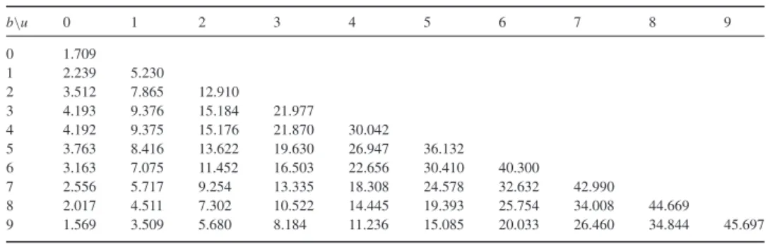
Table 6.2. Values ofV2(u,b)for 0≤u,b≤9.
b\u 0 1 2 3 4 5 6 7 8 9
0 1.709
1 2.239 5.230
2 3.512 7.865 12.910
3 4.193 9.376 15.184 21.977
4 4.192 9.375 15.176 21.870 30.042
5 3.763 8.416 13.622 19.630 26.947 36.132
6 3.163 7.075 11.452 16.503 22.656 30.410 40.300
7 2.556 5.717 9.254 13.335 18.308 24.578 32.632 42.990
8 2.017 4.511 7.302 10.522 14.445 19.393 25.754 34.008 44.669
9 1.569 3.509 5.680 8.184 11.236 15.085 20.033 26.460 34.844 45.697
C1 C2
= ⎛
⎜ ⎜ ⎝
d(eρ1uβ1(u)) du u=b
d(eρ2uβ2(u)) du u=b d2(eρ1uβ1(u))
du2
u=b
d2(eρ2uβ2(u)) du2
u=b ⎞
⎟ ⎟ ⎠
−1 ⎛
⎝
2V(b,b)
2+2
δ
c
V(b,b)
⎞
⎠.
The expressions forC1 = C1(b)andC2 = C2(b)are obtained in the same way as those for V(u,b).
Finally we get
V2(u,b)=C1eρ1uβ1(u)+C2eρ2uβ2(u),
and the table of values forV2(u,b)is as follows
The values on the table are identical to those obtained byAlbrecheret al.(2005).
7. Some concluding remarks
In this work we have shown, based on the techniques provided byLi(2008), a new method to find expressions for the distribution of the maximum severity of ruin in the Sparre–Andersen model with Erlang(n) interclaim times. Those expressions depend exclusively on the non–ruin probability and the claim amounts distribution.
In a Sparre–Andersen model with Erlang(n) distributed interclaim times, the expected times between claims are larger for higher values ofn, therefore the moments of the maximum severity of ruin are smaller.
The probability that the maximum severity occurs at the moment of ruin is bigger for higher values ofn. If we want to obtain similar explicit formulas for higher values ofn, the computations will become quite messy. However, we can still obtain numerical results using software like Mathematica.
In the case of Erlang(m) distributed claim amounts, the expected sizes of the claims are larger for higher values ofm, and therefore the moments of the maximum severity of ruin are also higher.
We generalized the results obtained byAlbrecheret al.(2005) to find the expected present value of dividends for any arbitrary claim amount distribution.
Acknowledgements
The authors gratefully acknowledge financial support from FCT-Fundação para a Ciência e a Tecnologia (Grant reference BD 67140/2009 and programme FEDER/POCI 2010).
References
Albrecher H., Claramunt M. M., & Mármol M. (2005). On the distribution of dividend payments in a Sparre–Andersen model with generalized Erlang(n) interclaim times.Insurance: Mathematics & Economics37, 324–334.
Bühlmann, H. (1970).Mathematical methods in risk theory. Berlin: Springer-Verlag. Dickson, D. C. M. (2005).Insurance risk and ruin. Cambridge University Press.
Dickson, D. C. M. & Waters, H. R. (2004). Some optimal dividends problems.Astin Bulletin34, 49–74.
Ji, L. & Zhang, C. (2011). Analysis of the multiple roots of the Lundberg fundamental equation in the PH(n) risk model. Applied Stochastic Models in Business and Industry.
Li, S. (2008). A note on the maximum severity of ruin in an Erlang(n) risk process.Bulletin of the Swiss Association of Actuaries, 167–180.
Li, S. & Dickson, D. C. M. (2006). The maximum surplus before ruin in an Erlang(n) risk process and related problems. Insurance: Mathematics & Economics38(3), 529–539.
Li, S. & Garrido, J. (2004). On ruin for the Erlang(n) risk process.Insurance: Mathematics & Economics34(3), 391–408. Picard, P. (1994). On some measures of the severity of ruin in the classical Poisson model.Insurance: Mathematics &
Economics14, 107–115.