ISSN 0104-6632 Printed in Brazil
www.abeq.org.br/bjche
Vol. 34, No. 01, pp. 307 - 316, January - March, 2017 dx.doi.org/10.1590/0104-6632.20170341s20140184
Brazilian Journal
of Chemical
Engineering
NUMERICAL RESEARCH ON THE
THREE-DIMENSIONAL FIBER ORIENTATION
DISTRIBUTION IN PLANAR SUSPENSION FLOWS
Qihua Zhang
*, Xiongfa Gao and Weidong Shi
National Research Center of Pumps, Jiangsu University,Zhenjiang 212013, People’s Republic of China. *E-mail: [email protected]
(Submitted: December 9, 2014 ; Revised: July 6, 2015 ; Accepted: September 19, 2015)
Abstract - To describe flow-induced fiber orientation, the Fokker-Planck equation is widely applied in the processing of composites and fiber suspensions. The analytical solution only exists when the Péclet number is infinite. So developing a numerical method covering a full range of Péclet number is of great significance. To accurately solve the Fokker-Planck equation, a numerical scheme based on the finite volume method is developed. Using spherical symmetry, the boundary is discretized and formulated into a cyclic tridiagonal matrix which is further solved by the CTDMA algorithm. To examine its validity, benchmark tests over a wide range of Péclet number are performed in a simple shear flow. For Pe=∞, the results agree well with the analytical solutions. For the other Pe numbers, the results are compared to results available in the literature. The tests show that this algorithm is accurate, stable, and globally conservative. Furthermore, this algorithm can be extended and used to predict the three-dimensional orientation distribution of complex suspension flows.
Keywords: Fiber suspension; Orientation distribution; Fokker-Planck equation; Finite volume; Planar flow.
INTRODUCTION
Fiber suspension flows are widely found in a va-riety of industrial applications, such as processing of thermoplastics, paper and pulp industries, etc. The final product is dependent on the microstructure of suspensions. Generally, a single fiber is affected by ambient fluid and nearby fibers. As a consequence, it changes the bulk flow rheological properties and leads to different macroscopic material behaviors. For instance, fiber orientation exerts potential effects on the physical properties of thermoplastic parts during molding, and distinctly determines the subse-quent stiffness, thermal conductivity, and mechanical behavior (Givler et al., 1983; Folgar and Tucker, 1984; Advani and Tucker, 1987).
For molding parts and paper sheets, the geo-metrical configuration is always very slim. By using
this feature, it is convenient to approximate the fiber suspension as a two-dimensional or planar flow. This approximation is widely recognized as the Hele-Shaw model, which was first adopted by Altan et al. (1990) to predict the three-dimensional orientation within channel and contraction flows. To improve computational efficiency, the quadratic closure approximation was used to close the orientation ten-sor or the moment of orientations originally pro-posed by Advani and Tucker (1987,1990). The clo-sure model approximates the higher order orientation tensor by lower order tensors, such as assuming
used by Larson (1999). Nevertheless, a closure model universally accurate for all types of flows is still not available.
In fact, fiber suspensions belong to a class of liquid type materials, which approach the equilibri-um state slowly compared to the changes within their microstructural configuration. Thus, the macroscopic properties are commonly induced by the flow. To describe this type of field configuration, the evolu-tion of the probability distribuevolu-tion funcevolu-tion is com-monly used and denoted by the Fokker-Planck equa-tion (Öttinger, 1996). However, the transient analyti-cal solution to this function only exists when the Péclet number is infinite (Pe=∞). Clearly, developing numerical techniques to solve this distribution func-tion is of great importance.
The distribution function provides a complete description of the orientation state. Therefore, the memory requirement is huge and the computation is time-consuming, especially in the early 1990s (Bay, 1991; Akbar and Altan, 1992). Consequently, the reduced two-dimensional model has been applied for a large variety of flows (Olson et al., 2004; Krochak et al., 2009; Chinesta et al., 2003). For a three-dimensional solution, there are only a few researches that have concerned the numerical methods, where the finite difference (Advani and Tucker, 1987; Kamal and Mutel, 1989) and the finite element (Strand et al., 1987; Han and Im, 1999) have mainly been employed. However, the solving procedure and the Péclet number range was not mentioned in Advani and Tucker 1987). The maximum Péclet number re-ported in Kamal and Mutel (1989) is 2×10⁴ and the maximum numbers are 60 and 100in Strand et al. (1987) and Han and Im (1999), respectively.
With modern computers, the numerical technique for directly solving the Fokker-Planck equation is feasible and necessary. In addition, in the past two decades, the finite volume method has been widely applied in molding process simulation and property analysis (Férec et al., 2008; Pei et al., 2012). In this paper, a numerical scheme based on the finite volume method is presented to solve the three-dimensional orientation distribution function. The numerical algo-rithm is tested by comparison with the analytical solution and data available in the literature, which covers the full range of Péclet number.
THEORETICAL FOUNDATION Fiber Orientation Distribution Model
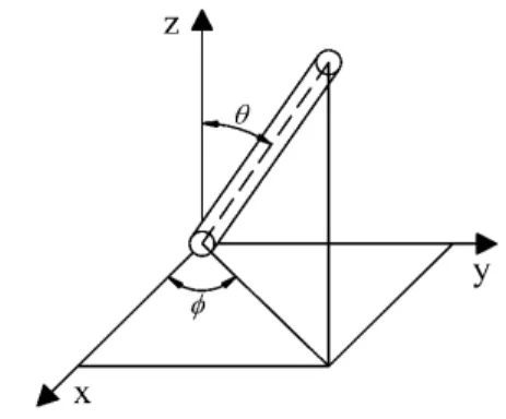
Using spherical coordinates, the fiber orien-tation is represented by a unit vector, i.e.,
1 2 3
= p p p, , sin cos ,sin sin ,cos
p , as shown
in Figure 1.
Figure 1: Schematic of a unit vector p. With millions of short fibers immersed in the sus-pensions, it is impractical to trace each fiber and to store its orientation state. An alternative is to adopt the stochastic process, where the fiber interactions are described by random collisions. On this basis, a statistical model was proposed by Folgar and Tucker (1984). Making use of this model, a probability dis-tribution function
p,t is defined to denote the probability to find a fiber located within the region [p,p+dp] at time t, and it can be written as
0 0 0 0
0 0 0
,
, sin
P d d
d d
(1)
The value of P is in [0,1]. Integrating the proba-bility distribution function over the orientation space, a normalization condition is formed as:
2
0 0
,t d , sin d d 1
p p
(2)Using the conservation principle in the orienta-tion space, the probability distribuorienta-tion funcorienta-tion must satisfy the continuity equation as
0t
p (3)
where is the gradient operator which refers to
p, p is the change rate of p and it can be written as:
E E:
p p p ppp (4)
where 1
2 T
u u
1 2
T
E u u is the strain rate tensor,
2 2
(rp 1) / (rp 1)
is the fiber shape factor, and
/ p
r L d is the fiber aspect ratio, i.e., the ratio of fiber’s length L to its diameter d. Eq. (4) is the well-known Jeffery equation (Jeffery, 1922).
To model the fiber-fiber interactions or Brownian motion in fiber suspensions, a random term Dr
is inserted into the right hand side of Eq. (4), and it becomes (Folgar and Tucker, 1984; Doi and Ed-wards, 1988; Dinh and Armstrong, 1984):
:
rD
D
E E
p p p ppp (5)
where Dris the rotary diffusion tensor and here is considered to be isotropic and replaced by a scalar
r i
D C which is called the rotary diffusivity (Folgar and Tucker, 1984), Ci is a constant describing the random interaction between fibers,
2
T
E
u u
is the shear rate tensor, and 1
: 2
is the effective shear rate.
Putting Eq. (5) into Eq. (3), the continuity equa-tion can be written as:
2r D t
p (6)
where
2 2
2
p is the Laplace operator. Eq. (6) is
the Fokker-Planck equation in fiber suspensions.
Constitutive Model of Fiber Suspensions
Based on the probability distribution function, it is convenient to apply statistical mechanics to the rheology of fiber suspensions. The macroscopic quantities of suspensions are expressed as the en-semble average of the corresponding quantities. For instance, for a tensor A p
, one has:
,t dA p
A p p p (7)where A p
is the macroscopic value of A p
. The moment tensor of orientation is a valuableprop-erty for the fiber suspensions. When
n
A p pp, the orientation tensor is:
,n n
t d
pp
pp p p (8)Based on the spherical symmetry, it is easy to write
,t ,t p p , that is, the function
p,t is an even function. For odd numbers of n, one has 0, 1,3,5
n
n
pp (9)
In the viewpoint of continuum mechanics, the fi-ber suspensions can be treated as the transversely isotropic fluid. On this basis, the constitutive equa-tion has been established by Ericksen (1960) and Hand (1962). Furthermore, the relationship between the stress and the rate of strain for dilute fiber sus-pensions has been described by Batchelor (1970) as:
1 1
2 f 3I
pppp pppp
(10)
where is the viscosity of the Newtonian fluid and f
is a function of fiber concentration, I is the second order unit tensor, and pppp and pp are, respec-tively, the fourth and second order orientation tensors.
Calculation of Orientation Tensors
Though the most complete description is pre-sented in the probability distribution function, only the orientation tensors are required to be known for the constitutive relationship Eq. (10). Moreover, the orientation tensors are symmetric, i.e., there are five independent components for pp (using the nor-malization condition: p12p22p321). Similarly, there are forty four independent components for
pppp .
Generally, the orientation tensors are calculated by the ensemble average with Eq. (8), where the probability distribution function is determined by solving the Fokker-Planck equation. An alternative method is to solve the evolution equation for the orientation tensors. Multiplying Eq. (6) by the tensor
2: r
d E E d D d
t
A p p
A p p p ppp p
A p p
(11)Taking the time partial derivative t
over the integral term
A p
dp, and noting the moment equationEq. (7), Eq. (10) becomes:
2: r
E E d D d
t
A p
A p p p ppp p
A p p (12)When A p
pp, and integrating the right hand side of Eq. (12) by parts, the evolution equation for the second order tensor is:
1
2 : 2 3
2 2 D Ir
t
pp pp pp pp pp pppp pp (13)
where the new term pppp appears, and an approximation is needed to close this equation. Using subscripts and denoting pp and pppp as aij and aijkl, respectively. The quadratic closure approximation is written as:
ijkl ij kl
a a a (14)
This model is rather simple and only accurate for a fully aligned orientation distribution. In addition, the linear approximation is
1
1
35 7
ijkl ij kl ik jl il jk ij kl ik jl il jk kl ij jl ik jk il
a a a a a a a (15)
The linear closure approximation is exact for an isotropic orientation distribution. To circumvent these limitations, many sophisticated models, such as orthogonal closure (Cintra and Tucker, 1995; Chung and Kwon, 2001), natural closure (Verleye and Dupret, 1993), etc., have been developed. The clo-sure model description is compact, general and easy to calculate, which is more widely used for fiber orientation characterization (Advani and Tucker, 1987). As we have seen, the closures are formulated by polynomials and their coefficients are determined by fitting data obtained from a variety of flow fields. In practice, users should be aware of the model characteristics and its applicable parameter range.
NUMERICAL METHOD
Dimensionless Form of the Fokker-Planck Equation
Substituting the nondimensional terms * / ,
* /
and tDr into Eq. (6), the dimension-less continuity equation can be written as:
* 2 Pe
p (16)
where the Péclet number Pe r D
is defined as the ratio of the effective shear rate to the rotary diffusivity.
Finite Volume Discretization
Integrating Eq. (16) over the orientation space, the integral equation is:
* 2Pe
V V V
dV dV dV
p
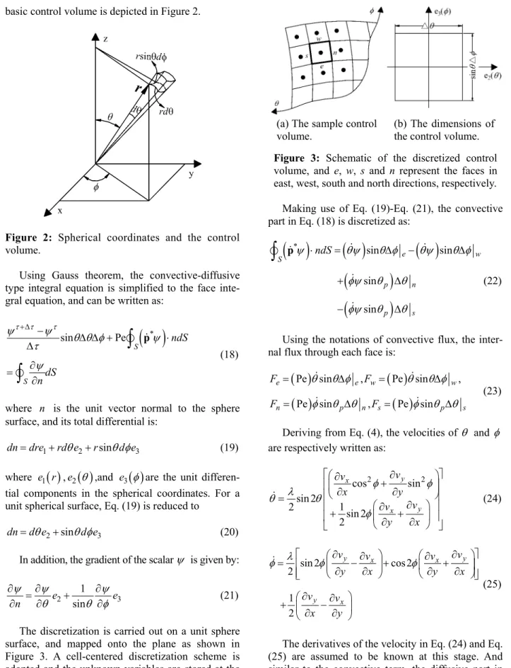
(17)basic control volume is depicted in Figure 2.
Figure 2: Spherical coordinates and the control volume.
Using Gauss theorem, the convective-diffusive type integral equation is simplified to the face inte-gral equation, and can be written as:
*sin Pe
S
S
ndS
dS n
p
(18)
where n is the unit vector normal to the sphere surface, and its total differential is:
1 2 sin 3
dndre rd e r d e (19)
where e r1
,e2
,and e3
are the unit differen-tial components in the spherical coordinates. For a unit spherical surface, Eq. (19) is reduced to2 sin 3
dnd e d e (20)
In addition, the gradient of the scalar is given by:
2 3
1 sin
e e
n
(21)
The discretization is carried out on a unit sphere surface, and mapped onto the plane as shown in Figure 3. A cell-centered discretization scheme is adopted and the unknown variables are stored at the solid points as shown in Figure 3(a).
(a) The sample control volume.
(b) The dimensions of the control volume.
Figure 3: Schematic of the discretized control volume, and e, w, s and n represent the faces in east, west, south and north directions, respectively.
Making use of Eq. (19)-Eq. (21), the convective part in Eq. (18) is discretized as:
*
sin sin
sin
sin
p
e wS
p n
p s
ndS
(22)
Using the notations of convective flux, the inter-nal flux through each face is:
Pe sin , Pe sin ,
Pe sin , Pe sin
e e w w
n p n s p s
F F
F F
(23)
Deriving from Eq. (4), the velocities of and are respectively written as:
2 2
cos sin
sin 2 1 2
sin 2 2
y x
y x
v v
x y
v v
y x
(24)
sin 2 cos 2
2
1 2
y x x y
y x
v v v v
y x y x
v v
x y
(25)
sin sin
1 1
sin sin
e wS
n s
p p
dS n
(26)
where the internal diffusive flux through each face is:
sin , sin ,
1 1
,
sin sin
e e w w
n n s s
p p
D D
D D
(27)
Then, putting Eq. (22)-Eq. (26) into Eq. (18), and the discrete algebraic equation can be written as:
1
1 1 1
1
P P P P P P
E E W W N N S S
E E W W N N
S S
a a a
a a a a
a a a
a
(28)
After rearrangement, Eq. (28) becomes:
1 1 1
1 1
P P E E
W W N N S S
E E W W N N
S S P P
a a a
a a a
a a a
a a a
(29)
where aE, aW, aS, aN and aP are coefficients listed in the Appendix. When 1 / 2, the Crank-Nicolson scheme is formed. To accelerate the convergence, the dimensionless time step is multiplied by a coefficient
, i.e., Dr, such that the time step can adapt to the varied Pe number.
Boundary Condition Implementation
On the sphere boundary, there are two pole points where singularity is always encountered because of
the term 1
sinp , while in the finite volume discreti-zation, this term is not directly evaluated on the
boundary. Alternatively, the flux is evaluated on the boundary instead of its value. In addition, it is easy to see that the flow area sin equals zero when
0
and , thus there is no flux through the boundaries of the two pole points. In the finite dif-ference discretization, the condition
0,
,
0 has been imposed on the boundary (Advani and Tucker, 1987; Kamal and Mutel, 1989), which means that there is no possibility that one fiber is located at these two pole points. Obviously, this condition is not always correct. Furthermore, the finite difference scheme does not guarantee the local flux conservation (Férec et al., 2008; Bay and Tucker, 1992). A finite volume scheme was provided by Bay (1991), Férec et al. (2008), Lin et al. (2010), Bay and Tucker (1992), but the implementation of the boundary condition was not detailed.
In practice, when 0 and 2 , the bounda-ries are joined together; thus, the spherical sym-metrical boundary condition is written as:
,0 ,2
(30) Assuming that the initial fiber orientation is iso-tropic, and using Eq. (2), one has:
2 0 0, sin d d 1
(31)That is,
, 1 / 4.The CTDMA Algorithm
Furthermore, Eq. (29) is discretized into a tridi-agonal matrix form, and at the control volume center (i, j), it can be written as:
, , , , 1 , , 1 ,
i j i j i j i j i j i j i j
A B C D (32)
where Ai j, a aP, Bi j, aN,Ci j, aS, and the other terms in Eq. (29) enter into Di j, . Similarly, at the cell center (i, j-1), assuming i j, -1
, 1 , , 1 ,1 , 1
i j i j i j i i j
E F G and inserting it into Eq. (32), and after rearrangement, the equation becomes:
, , , 1
, , , 1 , , 1 ,1, , 1 ,
i j i j i j i j i j i j i j i j i
i j i j i j
A C E B C F
C G D
(33)
, , , 1 , ,1 , i j
E
i j i jF
i j iG
i j
(34)Taking Ai j, C Ei j, i j, 1Ui j, , an iterative rela-tionship is obtained as:
, , , 1
, ,
, ,
, , 1 ,
,
,
, ,
i j i j i j
i j i j
i j i j
i j i j i j
i j
i j
B C F
E E
U U
C G D
E U (35)
At the boundary cell center (i, N), Eq. (32) becomes:
, , , , 1 , , 1 ,
i N i N i N i N i N i N i N
A
B
C
D
(36)And at the internal cell center (i, N-1), Eq. (34) becomes:
, 1 , 1 , , 1 ,1 , 1
i N Ei N i N Fi N i Gi N
(37)
Then inserting Eq. (37) into Eq. (36), leads to:
, , , 1
, , , 1, , 1 ,1
, , 1 ,
i N i N i N i N i N i N
i N i N i
i N i N i N
A C E B
C F
C G D
(38)
And similar to Eq. (37), Eq. (38) can be written as
, , , 1 , ,1 ,
i N Ei N i N Fi N i Gi N
(39)
Substituting Eq. (39) into Eq. (38), the expression for i N, 1 becomes:
, , ,, , , 1 , , , 1
, , 1 , , , 1 , ,1
, , 1 , , , , 1 ,
i N
i N
i N
i N i N i N i N i N i N
p
i N i N i N i N i N i N i
q
i N i N i N i N i N i N i N
m
A C E E B
C F A C E F
C G D A C E G
(40)
Then taking N 2 i k, and substituting the subscript i with k, Eq. (40) becomes:
, , ,
, , ,
, 1 ,1
, 1 ,1
i N i N i N
k N k N k N
i N i
k N k
p q m
p q m
(41)
On the boundary surface, Eq. (30) is:
, 1 ,1
, 1 ,1
i N k
k N i
(42)
Multiplying the first equation in Eq. (41) by
,
k N
p and noting
, ,1 , , 1
k N i k N k N
p
p
, it leads to:, , , , , ,
, ,
, 1 ,1
i N k N i N k N i N k N
k N i N
i N k
p p q q m p
m p
(43)
Thus, the boundary value is written as
, , , ,
, , , ,
, 1
i N k N k N i N i N k N i N k N
i N
m p m q p p q q
(44)
With Eq. (32), Eq. (34), Eq. (35), and using Eq. (44), the algebraic equation system can be iteratively solved by the LU decomposition, which has also been denoted as the cyclic tridiagonal-matrix algo-rithm (C-TDMA) (Férec et al., 2008; Bay and Tucker, 1992).
NUMERICAL CALCULATION AND VALIDATION
Test of Grid Relevance
To solve the time evolution of the probability dis-tribution function, there were 57 grids equally spaced in for the planar orientation (Advani and Tucker, 1987). The 39×77 grids were used in Advani and Tucker (1990), and the 40×40 grids were used in Férec et al. (2008) for the three-dimensional orienta-tion. But the accuracy validation, especially the grid relevance, has not been tested. In addition, for the transient Fokker-Planck, the calculation is computa-tionally-intensive using the high grid resolution. Alternatively, the steady Fokker-Planck equation is solved. Using Eq. (29) and noting 1, the steady discretization equation system is formed as:
0
P P E E W W N N S S
a a a a a (45)
several minutes to tens of minutes for 72×144, 144×288, 288×576 grids, but exceed ten hours for 1000×2000 grids. From Table 1, the error for 36×72 grids is rather big, so if the computational resources are enough, it is recommended to adopt high resolu-tion grids.
Table 1: Grid relevance test when Pe=100.
Grids/ a2 a11 a12 a22 36×72 0.730462 0.080243 0.094655 72×144 0.728071 0.076282 0.092953 144×288 0.727373 0.075166 0.092479 288×576 0.727188 0.074868 0.092354 1000×2000 0.727162 0.074659 0.091948 Analytical Solution When Pe=∞
When the Pe number is infinite, and the diffusion term is negligible in the Fokker-Planck equation, we obtain
t
p (46)
where the convection is dominant, and the analytical solution for the Fokker-Planck equation is (Dinh and Armstrong, 1984):
1
3/2, :
4 t t
p pp (47)
where E1, and E is the deformation gradient, calculated as
E
E E
t
p p (48)
When the fiber shape factor is unity, Eq. (48) becomes:
E
u E t
(49)
In a simple shear flow,
uy v, 0,w0
, and the shear rate is t, E can be written as:1 0
0 1 0
0 0 1
E
, and 1
1 0
0 1 0
0 0 1
E
.
Using Eq. (47)-Eq. (49), and noting Eq. (8), the time evolution for the orientation tensor is calcu-lated as
3/21
: 4
t ij
a d
pp
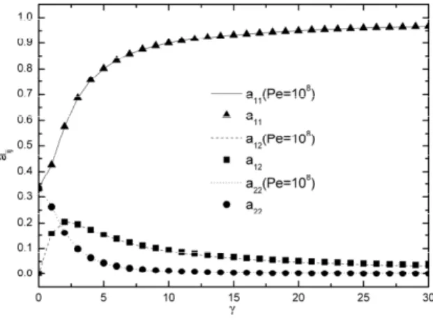
pp pp p (50)To test the numerical code with high Pe number, the main components a11, a12 and a22 are calcu-lated with 1000×2000 grids and compared to the analytical solutions (Pe=108), as shown in Figure 4. Comparison with Literature Results
For transient evolution of the orientation distribu-tion funcdistribu-tion, the calculadistribu-tion time becomes very long for high grid resolution. In the existing literature, the grid resolutions are 39×77 in Advani and Tucker (1990), 40×40 in Férec et al. (2008), or were not mentioned in Lin et al. (2010). So the calculation is carried on 36×72 grids and the results are listed and compared in Figure 5.
Figure 4: Comparison of the analytical solutions with Pe=108 (──a11, ……a12, and…………a22) and
the numerical results (▲ a11, ■ a12, and ● a22) for a
simple shear flow.
(b) a12 component vs. deformation
(c) a22 component vs. deformation
Figure 5: Comparison of numerical results adapted from the literature (Férec et al., 2008) (▲ Pe=1000, ■ Pe=100, ● Pe=10, and ◆ Pe=1) and the results in this
study (──Pe=1000, ……Pe=100,…………Pe=10,
and─…─…─Pe=1) for a simple shear flow.
By comparison, the main orientation tensors are in good agreement with the literature. The small dif-ference mainly comes from the grid resolution. For high Pe number, much more time is needed to reach the steady solution, so it manifests a big difference.
CONCLUSION
The objective of this research is to directly solve the orientation distribution function, i.e., the Fokker-Planck equation, which has been widely used in the prediction of fiber orientation distribution in fiber-filled polymers, pulp fiber suspensions, etc. To achieve this objective, a finite volume scheme is proposed. The scheme is characterized as globally conservative, accurate, and stable. Based on the face flux in the FV discretization, the singularity at pole
points encountered in the FD method is naturally solved. In addition, the global flux conservation is guaranteed. Then the spherical symmetry boundary condition is numerically formulated, which enhances the scheme’s accuracy. Subsequently, the numerical validation was conducted for a simple shear flow, where the results for Pe=∞ are compared with ana-lytical solutions, and the others are compared with data in the literature. Furthermore, this scheme is computationally inexpensive and suitable for the evaluation of the rheological properties of complex fiber suspensions.
ACKNOWLEDGMENT
The authors are grateful for the financial support by the National Natural Science Foundation of China (No. 51309118), the Natural Science Founda-tion of Jiangsu Province (No. BK20130527), and the Postdoctoral Science foundation of China (No. 2013M531282).
REFERENCES
Advani, S. G. and Tucker, C. L., Closure approxima-tions for three-dimensional structure tensors. J. Rheol., 34, 367 (1990).
Advani, S. G. and Tucker, C. L., The use of tensors to describe and predict fiber orientation in short fi-ber composites. J. Rheol., 31, 751 (1987).
Akbar, S. and Altan, M. C., On the solution of fiber orientation in two-dimensional homogeneous flows. Polym. Eng. Sci., 32, 810 (1992).
Altan, M. C., Subbiah, S., Güçeri, S. I. and Pipes, R. B., Numerical prediction of three-dimensional fi-ber orientation in Hele-Shaw flows. Poly. Eng. Sci., 30, 848 (1990).
Batchelor, G. K., The stress system in a suspension of force-free particles. J. Fluid Mech., 41, 545 (1970). Bay, R. S., Fiber orientation in injection molded
composites: A comparison of theory and experi-ment. PhD Thesis, University of Illinois at Urbana-Champaign (1991).
Bay, R. R. and Tucker, C. L., Fiber orientation in simple injection moldings. 1. Theory and numeri-cal methods. Poly. Com., 13, 317 (1992).
Chinesta, F., Chaidron, G. and Poitou, A., On the so-lution of Fokker-Planck equations in steady recir-culating flows involving short fiber suspensions. J. Non-Newt. Fluid Mech., 113, 97 (2003).
Cintra, J. S. and Tucker, C. L., Orthotropic closure approximation for flow-induced fiber orientation. J. Rheol., 39, 1095 (1995).
Dinh, S. M., Armstrong, R. C., A rheological equa-tion of state for semiconcentrated fiber suspen-sions. J. Rheol., 28, 207 (1984).
Doi, M., Edwards, S. F., Theory of Polymer Dynam-ics. Oxford University Press, England (1988). Ericksen, J. L., Anisotropic Fluids, Arch. Rat. Mech.
Anal., 4, 231 (1960).
Férec, J., Heniche, M., Heuzey, M. C., Ausias, G. and Carreau, P. J., Numerical solution of the Fokker-Planck equation for fiber suspensions: Applica-tion to the Folgar-Tucker-Lipscomb model. J. Non-Newt. Fluid Mech., 155, 20 (2008).
Folgar, F. and Tucker, C. L., A phonomenological model for concentrated fibre suspensions. J. Rei. Plas. Com., 3, 98 (1984).
Givler, R. C., Crochet, M. J. and Pipes, R. B., Nu-merical Prediction of fibre orientation in dilute suspensions. J. Com. Mat., 17, 330 (1983). Han, K. H. and Im, Y. T., Modified hybrid closure
approximation for prediction of flow-induced fi-ber orientation. J. Rheol., 43, 569 (1999).
Hand, G. L., A theory of anisotropic fluids. J. Fluid Mech., 13, 33 (1962).
Jeffery, G. B., The motion of ellipsoidal particles im-mersed in a viscous fluid. Proc. R. Soc. London, A102, 161 (1922).
Kamal, M. R. and Mutel, A. T., The Prediction of flow and orientation behavior of short fiber rein-forced melts in simple flow systems. Poly. Com., 10, 337 (1989).
Krochak, P. J., Olson, J. A. and Martinez, D. M.,
Fiber suspension flow in a tapered channel: The effect of flow/fiber coupling. Int. J. Multiphase Flow, 35, 676 (2009).
Larson, R. G., The Structure and Rheology of Com-plex Fluids. Oxford University Press, New York (1999).
Larson, R. G. and Doi, M., Mesoscopic domain theo-ry for textured liquid ctheo-rystalline polymers. J. Rheol., 35, 539 (1991).
Lin, J. Z., Zhang, Q. H., Zhang, K., Rheological properties of fiber suspensions flowing through a curved expansion duct. Poly. Eng. Sci., 50, 1994 (2010).
Olson, J. A., Frigaard, I., Candice, C. and Hämaläine, J. P., Modeling a turbulent fibre suspension flow-ing in a planar contraction: The one-dimensional headbox. Int. J. Multiphase Flow, 30, 51 (2004). Öttinger, H. C., Stochastic Processes in Polymeric
Fluids, Tools and Examples for Developing Simulation Algorithms. Springer, Berlin (1996). Pei, Z., Hu, B., Diao, C. and Yu, C., Investigation on
the motion of different types of fibers in the vortex spinning nozzle. Polym. Eng. Sci., 52, 856 (2012). Strand, S. R., Kim, S. and Karrila, S. J., Computation
of rheological properties of suspensions of rigid rods: stress growth after inception of steady shear flow. J. Non-Newtonian Fluid Mech., 24, 311 (1987).
Verleye, V. and Dupret, F., Proceedings of ASME Win-ter Annual Meeting. ASME, New York, 139 (1993). VerWeyst, B. E., Numerical Predictions of flow
in-duced fiber orientation in three-dimensional ge-ometries. PhD Thesis, University of Illinois at Urbana-Champaign (1998).
APPENDIX
5
5
5
5
max 0, 1 0.1 max ,0 ,
max 0, 1 0.1 max ,0 ,
max 0, 1 0.1 max ,0 ,
max 0, 1 0.1 max ,0 ,
, sin
E e e e
W w w w
N n n n
S s s s
P E W N S e w n s
a D Pe F
a D Pe F
a D Pe F
a D Pe F
a a a a a F F F F
a
,
,
, e e
e
w w
w
n n
n
s s
s F Pe
D
F Pe
D
F Pe
D
F Pe
D