INSTITUTO SUPERIOR DE ECONOMIA E GESTÃO

(1)

UNIVERSIDADE TÉCNICA DE LISBOA

INSTITUTO SUPERIOR DE ECONOMIA E GESTÃO

Master in Finance

Competitive Advantages as Source of Excess Stock Returns

Work by Nelson Miguel Jacinto Alves

Project with the supervision of MsC. Pedro Rino Vieira

Examiners:

Professor Raquel M. Gaspar

MsC. Pedro Rino Vieira

MsC. Inês Fonseca Pinto

(2)

Acknowledgements

I am eternally grateful to my parents, Victor and Celeste, and my brother Nuno, without their unconditional support and sacrifices this work would not be possible.

I would like to address a special thanks to my supervisor, MsC Pedro Rino Vieira, for his invaluable technical support, advice and endless patience in improving my writing. His help was crucial in making this work possible.

I would also like to thank to Professor Pedro Verga Matos for being a source of advice and guidance in critical times.

I want to express my gratitude to Diogo Rebelo for being a source of invaluable motivation that has been an inspiration since high-school.

I would like to thank Alexandre Antunes for being a source of valuable ideas and moral support.

I also would like to thank Luís Dias, Eduardo Veríssimo and João Pereira. Their professional collaboration meant a great deal to me.

I would like to acknowledge the contributions of Ana Paula Carvalho and Hugo Oliveira for their comprehensiveness and support. I would also like to acknowledge BES (Banco Espiríto Santo) for letting me use the Bloomberg database so useful in this work.

Finally, a special thanks to my friends always supportive of my work . Special Thanks to João Hipólito and Cláudia Luzio for the help in the preparation of my defense.

(3)

Resumo

A avaliação das perspectivas para uma determinada empresa é um passo critico no processo de valorização de uma acção. Uma correcta avaliação resulta na definição de um conjunto de pressupostos que levarão a uma avaliação mais precisa. Analises erradas levam a conclusões erradas e são resultado da falta de um quadro orientador que direccione o estudo das perspectivas das empresas em causa. Para resolver este problema decidimos recorrer à teoria da gestão estratégica e testar a relação entre rendibilidades de acções e Vantagens Competitivas relevantes em determinada indústria. Aplicámos este método à Industria Siderúrgica e realizamos testes estatísticos. Os resultados mostram-nos que, na generalidade, melhorias na eficiência operacional, medida através das primeiras diferenças da margem bruta, oferece retornos acima da taxa de retorno sem risco. Estes resultados mostram-nos que a selecção de portfolios, utilizando Vantagens Competitivas, permitem-nos obter retornos acima da média.

Palavras-chave: Valorização; Gestão Estratégica; Industria Siderúrgica; Margem Bruta; Vantagens Competitivas, CAPM, Teoria da Carteira, Cross Section Rrturns

(4)

Abstract

The perspectives assessment of any given company is a vital step to the efficiency of the valuation process. A correct assessment will result in the definition of assumptions that will lead to better valuation results. Wrong conclusions are frequently taken because a bad assessment was made and this is the result of the lack of a proper framework that guides the analysis of company perspectives. To solve this problem we decided to use strategic management theory and test the relation between stock returns and competitive advantages relevant for a given industry. We applied this method to the Steel Industry and tested it statistically. The results showed us that, generally, improvements in the operational efficiency, measured by the first differences in gross margin, provide excess returns. This results show us that the use of Competitive Advantages to select portfolios, in the Steel Industry, yields better than average returns.

Key words: Valuation; Strategic Management; Steel Industry; Gross Margin; Competitive Advantages, CAPM, Portfolio Theory, Cross Section Returns

(5)

Index of Tables

Table 1 - Expected CA impact on stock returns ... 13

Table 2 - Summary Statistics ... 18

Table 3 - Model 1: Pooled OLS ... 20

Table 4 - Model 2: Random Effects GLS ... 21

Table 5 - Model 3: Fixed-Effects GLS Before Crisis ... 23

Table 6 - Model 4: Pooled OLS During Crisis ... 24

(7)

Index of Figures

Figure 1 - Dependent Variables ... 19

(8)

1

1 - Introduction

In the genesis of this work is the desire to offer a new and complementary perspective to the security analysis framework.

Today, in the financial markets, stock analysts usually look for “fundamentals” and then try to assess potential growth. An asset manager might add, to this assessment, parts of the portfolio theory. We can divide the stock selection process in three parts: valuation, perspectives assessment and portfolio construction (Chugh and Meador, 1984). The weakest part in the mentioned process is the perspective assessment, mainly because, to our best knowledge, there is not any coherent framework for securities analysis of firm’s growth potential (Cottle, Murray and Block, 1988). Our goal with this work is to make some progress in the right direction trough the development of an integrated initial framework that is in accordance with both valuation theory, portfolio theory and strategic management. In this work we will define relevant Competitive Advantages (CAs) for the Steel Industry and perform an analysis of its impact on stock returns. We should state the reasons that led to the choice of the Steel Industry as base case for our study. The Steel Industry has a long history, this means that many sources of information already exist. Also many studies were made about this industry and its conclusions are usually extremely similar in relation to the CAs present in this work. This will help us avoid controversy related with the choice of the CAs. Other advantage is the fact that exists a long database of companies in this industry with crucial information, which will allow us to make the work credible from the statistical perspective.

In the Strategic Management literature, Competitive Advantages are related with above average profits, which in accordance with valuation theory should mean above average investment returns (Porter, 1985). Our results suggest that there is a positive relation between Competitive Advantages and stock returns. For example we found that during the period of the study Low Costs Achieved are source of excess returns. We also tested for the period before the crisis and during the crisis. The results are very interesting.

(9)

2 Advantages. The theoretical background related with competitive advantages will be explored in section 3. Our focus will be on Competitive Advantages applicable to our case. Following this, we will construct a model based in the theoretical foundations built in sections 2 and 3. This will consist in the model, in section 4, designed to capture the effects of Competitive Advantages and also to control for known drivers of stock returns. In section 5, we will show and explain the results obtained. In section 6 we will comment on the main limitations and problems involved in the making of this work. We will finish in section 7, with our conclusions and insights for future research.

2 - Cross-Section Returns

2.1 - Historical Context

The middle of the 20th century brought new theories to the fields of investments, portfolio selection and diversification. Markowitz (1952, 1959) is one of the examples of academics with new findings in this areas.

However in the beginning of the 60’s there was still a lack of a microeconomic theory dealing with conditions of risk (Sharpe, 1964). At the time academics theorized about the idea that, if rational, one investor should be able to reach any point in the capital market line. This way he can only obtain a higher return if he incurs in additional risk. Therefore, the price of the investment can be divided in two parts: the price of time and the price of risk (the expected additional return per unit of return of risk incurred).

Markowitz (1952, 1959) stated that an investor should consider portfolio return as a desirable thing, and return variance as an undesirable thing. Following this logic he concludes that an investor should pursue a set of efficient portfolios that maximize returns for a given variance. This way, under certain conditions, it should be possible for an investor to setup an optimum portfolio of risky assets and then allocate his funds between this risky portfolio and risk-free assets. Therefore, the investor is capable of defining the level of risk with which he is comfortable (Tobin, 1958).

(10)

3 Sharpe (1964) concluded that there is a relationship between expected returns and systematic risk. This author stated that the return on a given asset i, included in an optimal portfolio g, will be heavily related with the return on the portfolio g, Sharpe called this systematic risk. The specification of a relation between the returns of i and g allows the utilization of a predictive model.

The usual proceeding is to perform the regression of the returns of any given security against its benchmark. Sharpe (1964), Lintner (1965) and Black(1972) introduced the asset pricing model based on the assumption that expected returns on a security are sensitive to the market return, commonly known as market . In other words, expected returns are a positive linear function of the slope of the security’s returns on the market’s return regression, and the ’s are enough to provide a description of the cross-section of average returns (Fama and French, 1992). The central idea was that the market portfolio is mean-variance efficient in the way Markowitz (1959) described it.

The model was commonly known as the Sharpe-Lintner-Black (static) Capital Asset Pricing Model (CAPM), and was defined as:

1 1 0

]

[R_i =

γ

+

γ

β

E ,

Where: ] [Ri

E is defined as the expected on any asset i,

1 0,

γ

are the coefficients of the regression,

1

β

is defined as

] [ / ) , (

1 =Cov Ri Rm Var Rm

β

,

Where: ) , (R_i R_m

Cov is the covariance between R_i,R_m, ]

[R_m

Var is the variance of R_m,

(11)

4 (1981) examined the relation between returns and size (total market value) of a group of stocks, and concluded that smaller firms had more risk, on average, than larger firms. Basu (1983) tested the effect of firm size and earnings to price ratio (earnings’ yield) with stock returns. His results confirm that stocks with high E/P ratio earn, on average, higher risk adjusted returns. This effect is not independent of firm size. Bhandari (1988) concluded that the expected stock returns positively related with financial leverage when controlling for market and firm size. As shown by these authors numerous factors not included in the capital asset pricing model (CAPM) of Sharpe (1964), Lintner (1965) and Black (1972) are relevant in explaining stock returns. These patterns are called anomalies.

This way, Fama and French (1992) concluded that if the market is rational then stock risks are multidimensional, and might be proxied by this different dimensions. The study of these anomalies resulted in Fama and French (1993) multifactor model

2.2 - Fama-French Multifactor Model

The FF (1993) multifactor model captures most of this effects. Fama-French multifactor model states that the expected return on a portfolio in excess of the risk-free rate is explained by the sensitivity of the return to three factors: the market return, the size of the company, and the book-to-market ratio of the company. The conceptual model is the following:

) ( ) ( ] ) ( [ )

(R R b E R R s E SMB hE HML

E i − f = i m − f + i + i ,

Where:

f i R

R

E( )− is the expected return on a portfolio in excess of the risk-free rate;

f m R

R

E( )− is the expected excess return on a broad market portfolio;

)

(SMB

E is the expected difference between the return on a portfolio of small stocks and the

return on a portfolio of large stocks (SMB, small minus big).

)

(HML

E is the expected difference between the return on a portfolio of high-book-to-market

stocks and the return on a portfolio of low-book-to-market stocks (HML, high minus low).

i

(12)

5

Fama-French (1995), found that the book equity to market equity ratio (BE/ME) captured a

significant part of the cross-section of average returns. The authors theorized that systematic

differences in returns are caused by differences in risk. Therefore, if stocks are priced

rationally, then size (Market Equity) and BE/ME can be a good proxy for sensitivity to

common risk factors in returns. Fama-French (1995), demonstrated that portfolios

constructed to capture risk factors related to ME and BE/ME explain a significant amount of

the variation in stock returns.

In the same article, the authors provide an economic theory to justify the above relation. The

main idea is that low BE/ME is a characteristic of firms with high average return on capital,

and high BE/ME is typical of distressed firms, therefore investors will demand higher

expected returns from distressed firms because of the extra risk. At the same time, after

controlling for BE/ME, size tends to be positively correlated with earnings on book equity,

although this last relation was not significant until 1980.

Summarizing, Fama-French multifactor model explains the cross-section variation in

expected returns, because pricing rationality implies that differences in average returns are

related to differences in risk, then ME and BE/ME must proxy for sensitivity to common risk

factors in returns.

2.3 - Fama-French Multifactor Model Criticism

After Fama and French published their set of articles sustaining the multifactor model some

criticism arose.

Lakonishok, Shleifer, and Vishny (1994) defended that the high returns originated in high

book-to-market stocks (value stocks) are the result of an incorrect pricing by investors that

presume that past earnings growth rates of low book-to-market stocks (growth stocks) will

continue in the future. What happens is an over discount of future earnings of growth stocks,

and an under discount of value stocks that later will produce high returns on the latter. Other

explanation offered by Lakonishok, Shleifer, and Vishny (1994) is that growth stocks are

more attractive to less experienced investors who drive the prices higher, therefore lowering

the expected returns of the stocks.

Daniel and Titman (1997), argued that the prevailing literature focused on the debate whether

(13)

6

authors question the possibility of ME/BE and ME are associated with risk factors, and if

there is any risk premium related to these factors. They concluded that: “(1) there is no

discernible separate risk factor associated with high or low book-to-market (characteristic)

firms, and (2) there is no return premium associated with any of the three factors identified

by Fama and French (1993).” Daniel and Titman (1997, p. 3). The results obtained suggest

that the high returns originated cannot be interpreted as compensation for risk factor. The

main reason to the existence of significant covariance between high book-to market stocks is

not the presence of particular risks associated with distress, but the fact that this stocks

usually have similar properties. The characteristics might be related lines of business, same

industry or geographical region.

Therefore in the development of this work we will use Daniel and Titman (1997) assumption

that the factors in the Fama-French multifactor model are in fact proxies for firm

characteristics, and not risk factors. This way we will be able to avoid the criticism

mentioned and we will be testing firms characteristics that might affect returns. Since we are

looking for characteristics that provide above average returns and firm characteristics are the

bundle of resources and capabilities that exist within a company, we are in fact testing for

interactions that can provide competitive advantage.

3 - Competitive Advantages in the Steel Industry

3.1 – Historical Context

In the first decades of the last century, economists have focused in the conceptualization of a

framework for the treatment of the financial markets. Two main views were prevalent, one

sustained that the long-term estimation of investment value is on average fruitless because the

people practicing it do not have enough weight on the market (Keynes, 1935). Other view

sustained that if you calculated correctly the intrinsic value of any investment, and if you buy

it at a price below its intrinsic value, then you would never lose money (Williams, 1938).

Keynes (1935, p. 130) argued that “(…) professional investment may be likened to those

newspaper competitions in which the competitors have to pick out of six prettiest faces from

(14)

7

corresponds to the average preferences of the competitors as a whole; so that each competitor

has to pick, not those faces which he himself finds the prettiest, but those which he thinks

likeliest to catch the fancy of the other competitors, all of whom are looking at the problem

from the same point of view. It is not a case of choosing those which to the best of one’s

judgment, are really the prettiest, nor even those which average opinion genuinely thinks the

prettiest. We have reached the third degree where we devote our intelligences to anticipating

what average opinion expects the average opinion to be. And there are some, I believe who

practice the fourth, fifth and higher degrees.”

The author argues that it might prove better for an investor to follow the crowd than to enter

laborious work trying to forecast investment value and to expect that the future proves him

right.

John Burr Williams (1938) argued that the present worth of cash-flows is the critical factor in

buying stocks. If an investor buys a security below its investment value, he will never lose

even if the price falls at once, because he can always hold for income and get an above

normal return on his price cost. Williams (1938) developed the mathematical foundations for

investment analysis. However, the greatest problem on his theory, is that it is heavily

dependent on the assumptions for certain variables, which is the real risk in his model: the

risk of having wrong assumptions.

Fisher (1958) would use much less calculations on his valuations, putting the emphasis on

getting the assumptions right. He would look for a set of characteristics, in a company, that

would reduce the uncertain about the assumptions set, usually growth prospects, and

profitability. Fisher (1958) advised looking for firms with low-cost production; strong

marketing organization; outstanding research and technical effort; financial skills; flexible,

motivated and creative human resources; and always check for the industry characteristics.

Porter (1985) brought to the public the concept of sustainable Competitive Advantage

(hereafter CA). The characteristics mentioned in the last paragraph can easily be classified as

drivers of CA as they are defined by Porter (1985). To the same effect Porter (1985) also

stated that the presence of competitive advantage was a source of above average returns.

This way, returning to Williams (1938), one can argue that if the presence of competitive

advantages will result in higher cash-flows with less uncertainty, the assumptions defined by

Williams’ model will be more robust, and at the same time the investment return calculated

(15)

8

This work intends to provide further insights to this discussion, and to identify potential tools

that allow to test the theory developed trough this work.

In the following sections we carefully select a set of Competitive Advantages (CA) that we

consider that can be used in the study of the Steel Industry.

3.2 - Competitive Advantages Definition

Before we progress in our work we should remark that CA is a critical concept in strategic

management. However there is not one widely accepted definition, instead there are many

definitions. In the context of our work, we think that the following three definitions are the

most relevant:

i) Competitive Advantage “is a factor or an effect which permits one participant in a

business to offer a product or service more effectively than competitors.” Carroll

(1982, p. 10).

ii) “Competitive advantage grows fundamentally out of the value a firm is able to create

for its buyers that exceeds the firm’s cost of creating it.” Porter (1985, p.3).

iii) Competitive Advantage “is the unique position an organization develops vis-à-vis its

competitors through its patterns of resource deployments.” Hofer and Schendel

(1978, p.25).

Porter (1985) defines two main alternatives strategies to achieve success: cost leadership or

differentiation. This way every driver of competitive advantage must be a positive influence

for one of these two types of strategies.

Veríssimo (2004) defined a set of competitive advantage drivers. We decided to choose the

CAs from that set for our research, with some modifications that better suite our specific

work. The set of drivers adopted was chosen in accordance with the management theory on

(16)

9

3.3 – The Steel Industry and its Competitive Advantages

The steel industry is characterized by its capital intensive nature. Therefore fixed costs

perform an important role in the management of this units. Usually mills try to operate close

to full capacity in order to dilute their fixed costs. Thompson and Strickland (1992), argued

that cost efficiency is a critical factor to achieve success, mainly because the majority of steel

products are in fact commodities, therefore the price is the main decision factor for buyers.

There are two CAs associated with productive efficiency in the set designed by Veríssimo

(2004): Economies of Scale and Low Costs Achieved.

Thompson and Strickland (1992) also emphasized that constant improvements are

determinant to the success of steel mills, mainly because these improvements result in

increased output, faster operations, higher quality, and lower costs. Usually cost-saving and

efficiency enhancements are executed trough capital expenditures (Capex) which are used to

implement cutting edge technology. This indicates that innovation is very important to the

steel industry. In the same work Thompson mentions interviews with Steel executives where

it is mentioned the fact that the Steel Industry is extremely dependent of economic cycles,

which force them to be prepared for bad times through the maintenance of good financial

strength in order to maintain the ability to invest even in bad times.

Following Thompson’s analysis of the Steel Industry, we think that we should test for: Low

Cost Achieved, Economies of Scale, Innovation, and Financial Strength and Financial Skills.

Additionally we will control for Market Risk ( ), Size and BE/ME ratio, as Fama-French

suggested, but in the perspective used by Daniel and Titman (1997), as we stated before.

3.4 - Selected Drivers of Competitive Advantages

For the case studied in this work we decided to select the following drivers of CA from the

set provided by Veríssimo (2004). Our choice is justified by the applicability of these CA to

the case in study, as addressed before.

3.4.1 - Economies of Scale

In general terms, we can say that economies of scale exist when fixed costs are much higher

(17)

10

companies are able to amortize the fixed costs over greater volumes, condemning small

competitors to play the game on a adversely sloped field (Christensen, 2001).

Porter (1985) observed that cost advantage will result in above average performance only if a

firm can sustain it in order to create a key entry/mobility barrier. A firm can do that by

increasing advertising spending, increase spending to boost the rate of technological change,

shorter model life cycles where models require fixed or quasi-fixed development costs,

increase sales force or service coverage. Since large scale is the factor that allows an activity

to be performed in an unique way that is not possible at a smaller volume, competitors will

have huge costs to replicate the strategy, mainly because he will have to buy market share. In

order to test these driver of CA we will use Total Sales as a proxy for Economies of Scale.

Total Sales has been used as proxy to capture economies of scale by many authors such as

Rugman and Verbeke (2007).

Assumption 1: Economies of Scale are properly represented by Total Sales as reported in the

firm’s financial statements.

Hypothesis 1:

H0: Economies of Scale are not significant

3.4.2 - Low Costs Achieved

Porter (1985) argued that low cost is one source of competitive advantage a firm may

possess. The author presented the following 10 cost drivers as the main determinant of cost

performance: economies of scale; learning and spillovers; the pattern of capacity utilization;

linkages; interrelationships; integration, timing; discretionary policies; location; and

institutional factors. The mentioned cost factors can be more or less under a firm’s control.

Day and Wensley (1988) identified lower relative costs as a positional advantage. It occurs

when a firm is able to perform most activities at a lower cost than competitors. They have

used the example of Nucor, which by using scrap metal instead of iron ore achieved cost

advantage.

If used efficiently, low cost position, allows a firm to earn above average returns in spite of

strong competitive forces such as: rivalry within the industry, bargaining power of buyers,

bargaining power of suppliers, potential entrants, and product substitutes (Ireland et al, 2007).

(18)

11

manufacturing and distribution process. McConaugby, Matthews and Fialko (2001) used

Gross Margin as proxy for operational profitability.

Assumption 2: Low Costs Achieved is properly represented by Gross Margin as reported in

the firm’s financial statements.

Hypothesis 2:

H0: Low Costs Achieved are not significant

3.4.3 - Financial Strength and Financial Skills of an Organization

The basic financing of any merchant operation is vital to its survival. In the absence of

working capital the operation would be financially struggled and with no initial capital to

initiate the venture the company would never exist in the first hand. Thus every firm needs to

possess financial basic skills.

Ireland et al (2007) went further in detail and enhanced two main financial resources: the

firm’s borrowing capacity, and the firm’s ability to generate internal funds. The authors also

mention financial ability as a resource vital to achieve competitive advantage either when the

industry is capital intensive or when pursuing growth opportunities.

Efficient Market Hypothesis, Fama (1970), has been used to defend the idea that every good

business will find financial back up in the capital market. However, EMH has been criticized

in the last years and several anomalies have been spotted (Myers and Brealey, 2003). Even if

the EMH holds, imperfections arise that will disturb the optimal capital allocation. Barney

(1986) argues that when few firms have the financial backing to acquire strategic factors,

since there are no perfect competition dynamics, then there will be opportunities to achieve

above average returns. Thus the corporation’s financial strength serves has source of

competitive advantage. Capital markets will prefer to apply its capital in established firms,

avoiding the uncertainty of newcomers, Barney (1986). This way the market will rely on the

reputation of established corporations with a solid balance sheet. The ultimate case would be

the one where the capital markets would apply resources in a newcomer but at one risk

premium rate that would put the newcomer at a financial disadvantage.

Myers and Brealey (2003), also mention the ability to allocate financial resources in the

(19)

12

mentioned that long-term debt to total equity ratio is a measure of financial strength widely

used in the Steel industry.

Assumption 3: Long-term debt to total equity ratio represents properly the Financial Strength

and Financial Skills of an organization.

Hypothesis 3:

H0: Financial Strength and Financial Skills of an organization are not significant

3.4.4 - Innovation

Innovation is “the acceptance and implementation of new ideas, processes, products and

services.” (Thompson, 1965, p.1).

Drucker (1998 p.149) states that innovation “(…) is the means by which the entrepreneur

either creates wealth-producing resources or endows existing resources with enhanced

potential for creating wealth.”

Hurley & Hult (1998) further divide innovation in two different stages: i) Innovativeness:

which is the openness of a company’s culture toward innovation, and ii) capacitytoinnovate:

that is the ability of a given organization to implement new ideas in its processes or products.

Many organizational theorists defend that innovation has sources inside and outside the

company. Drucker (1998) highlights as main internal sources of innovations: unexpected

occurrences, incongruities, process needs, industry and market changes, and as main external

sources of innovation: demographic changes, changes in perception and new knowledge.

In general, organizations that possess capacity to innovate are able to develop competitive

advantages and generate higher levels of performance. Reichstein and Salter (2006) used

Capex-to-Sales ratio as proxy for innovation.

Assumption 4: Innovation is properly represented by Capex-to-Sales ratio as reported in the

firm’s Financial Reports

Hypothesis 4:

H0: Innovation is not significant

(20)

13

Table 1 - Expected CA impact on stock returns

This table presents the proxies of the Competitive Advantages and its expected effect on stock returns

Competitive Advantage Proxy Expected Effect on Stock Returns

Economies of Scale Total Sales +

Low Costs Achieved Gross Margin +

Financial Strength and Financial Skills

Long Term Debt-to-Total

Equity ratio -

Innovation Capex-to-Sales ratio +

4 - The Model

4.1 - Data

We used all firms in Bloomberg World Steel Index, which was taken from the Bloomberg

database. All companies which do not have complete data for the period were excluded, in

order to have a balanced panel data in which every company has one observation for each

year. This will allow us to follow the evolution of the performance of the companies during

the entire period, and avoid the problems associated with unbalanced panels. This resulted in

the formation of a database of 40 companies (Annex 1) for 7 years, from 2004 to 2010. We

chose this period range because the Bloomberg World Steel Index does not have any

historical record before these dates. In the date range we have 4 years of economic growth

and 3 years of economic recession, we think that this data covers a wide range of scenarios,

good and bad, which adds value to the study. Actually, this will allow us to test the impact of

the subprime crisis. Also the theory in panel data suggests that 7 years is enough for the study

to be credible. We used gretl 1.9.5cvs software to do the statistical analysis. The data was

organized as panel data. We will use the models suitable to this kind of data, such as the

(21)

14

4.2 – Model

The variables:

ft pt R

R − is the dependent variable, and corresponds to the difference between the stock

returns of company p and the EURIBOR1 12 months interest rate for year t. In this case we

used the returns, and risk free returns for each year starting in the 1st of April of each year.

We justify this action with the fact that all the companies usually take the first three months

of the year to present its annual results, therefore we have to cover the gap between the end of

the fiscal year, and the presentation of the information to the public. Fama and French (1992)

used a similar procedure for their work, but in their case they used 6 months. We think that

the companies present in our sample are in position to present their financial information to

the public until the end of the 1st quarter, additionally we think that if we were to follow

Fama-French period of 6 months, we would be creating a bias because most of the companies

observed are prominent companies that disclose financial information quarterly. So we would

be capturing returns that would be affected by the information of the 1st quarter of the

following year, this way undermining our results.

ft mt R

R − is the difference between the market returns and the risk free returns for year t,

starting in the 31st of March. The benchmark used is the Bloomberg Europe 500 Steel

Industry.

Hypothesis 5:

H0: We accept that Rmt −Rft is not statistically different from zero

H1: We do not reject that R_mt −R_ft is statistically different from zero

pt

SIZE

LN_ is the natural logarithm of the Market Capitalization of the company p in the

year t. We use the natural log because we think that best represents the behaviour of the

variable.

1

(22)

15

Hypothesis 6:

H0: We accept that LN_SIZEptis not statistically different from zero

H1: We do not reject that LN_SIZE_ptis statistically different from zero

pt

BEME is the Book Equity to Market Equity ratio of company p in the year t .

Hypothesis 7:

H0: We accept thatBEME_ptis not statistically different from zero

H1: We do not reject that BEME_ptis statistically different from zero

pt

GROSS is the Gross Margin ratio of company p in the year t. With this variable we expect

to control for the CA Low Costs Achieved.

Hypothesis 8:

H0: We accept that GROSS_pt is not statistically different from zero

H1: We do not reject that GROSS_pt is statistically different from zero

pt

dGROSS is the first difference of GROSS_pt of company p in the year t. With this variable

we want to control for improvements in Low Costs Achieved.

Hypothesis 9:

H0: We accept that dGROSS_pt is not statistically different from zero

H1: We do not reject that dGROSSpt is statistically different from zero

pt

LTDTTE is the Long Term Debt to Total Equity of company p in the year t. With this

variable we want to control for Financial Strength and Financial Skills.

Hypothesis 10:

(23)

16

H1: We do not reject that LTDTTEpt is statistically different from zero

pt

LTDTTE

sq_ is the square of ratio of company p in the year t. We used this setup because,

theoretically, as the LTDTTE ratio increases it will have a positive effect in the returns, but as

the LTDTTE increases to large levels, then it will start to have a marginal negative impact in

the company.

Hypothesis 11:

H0: We accept that sq_LTDTTEpt is not statistically different from zero

H1: We do not reject that sq_LTDTTE_pt is statistically different from zero

pt

SALES

LN_ is the natural logarithm of the sales of company p in the year t. This variable

represents the impact of Economies of Scale in the returns of the stocks returns. Again we

used the natural log since it makes theoretical sense and it best represents the behaviour of the

variable.

Hypothesis 11:

H0: We accept that LN_SALES_pt is not statistically different from zero

H1: We do not reject that LN_SALES_pt is statistically different from zero

pt

CAPEXSAL

LN_ is the ratio of capex to sales ratio of company p in the year t. With this

variable we want to capture the impact of innovation on stock returns. Our interpretation is

that the natural log is the better way to represent the impact of the variable because the in

some cases the Capexsal ratio has a disproportioned size due to the impact of sales collapse

during the crisis, and not because of the reinforcement of the investment in innovation. This

way we decided to use the logarithm to smooth this effect on the variable.

Hypothesis 12:

H0: We accept that LN_CAPEXSAL_pt is not statistically different from zero

(24)

17

CRISIS is a dummy variable that controls for the effect of the Subprime crisis. CRISIS is 1

in the years of 2008, 2009 and 2010, and 0 otherwise.

Hypothesis 13:

H0: We accept that CRISIS is not statistically different from zero

H1: We do not reject that CRISIS is statistically different from zero

The variables mentioned will be studied in the following model:

(25)

18

5 – Results

From the data available we obtained the following descriptive statistics:

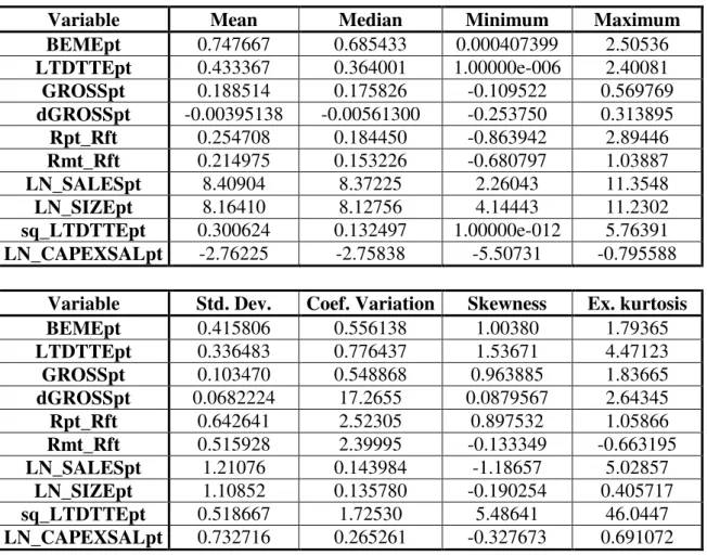
Table 2 - Summary Statistics

This tables present the results obtained for the descriptive statistics for all the variables studied. We included the results for the mean, median, minimum, maximum, standard deviation, coefficient of variation, skewness,

and kurtosis. We excluded the variable CRISIS because due to the fact that it is a dummy variable and its results

are meaningless.

Variable Mean Median Minimum Maximum BEMEpt 0.747667 0.685433 0.000407399 2.50536

LTDTTEpt 0.433367 0.364001 1.00000e-006 2.40081

GROSSpt 0.188514 0.175826 -0.109522 0.569769

dGROSSpt -0.00395138 -0.00561300 -0.253750 0.313895

Rpt_Rft 0.254708 0.184450 -0.863942 2.89446

Rmt_Rft 0.214975 0.153226 -0.680797 1.03887

LN_SALESpt 8.40904 8.37225 2.26043 11.3548

LN_SIZEpt 8.16410 8.12756 4.14443 11.2302

sq_LTDTTEpt 0.300624 0.132497 1.00000e-012 5.76391

LN_CAPEXSALpt -2.76225 -2.75838 -5.50731 -0.795588

Variable Std. Dev. Coef. Variation Skewness Ex. kurtosis BEMEpt 0.415806 0.556138 1.00380 1.79365

LTDTTEpt 0.336483 0.776437 1.53671 4.47123

GROSSpt 0.103470 0.548868 0.963885 1.83665

dGROSSpt 0.0682224 17.2655 0.0879567 2.64345

Rpt_Rft 0.642641 2.52305 0.897532 1.05866

Rmt_Rft 0.515928 2.39995 -0.133349 -0.663195

LN_SALESpt 1.21076 0.143984 -1.18657 5.02857

LN_SIZEpt 1.10852 0.135780 -0.190254 0.405717

sq_LTDTTEpt 0.518667 1.72530 5.48641 46.0447

LN_CAPEXSALpt 0.732716 0.265261 -0.327673 0.691072

The analysis of the main statistics provides us a good picture of the data available. The results

show that the sample chosen provides a wide range of observations that will offer robustness

to the results obtained. For each variable the mean assumes expected standard values. For

example BEMEpt has a 0.75 mean, GROSSpt has a 0.18 mean and LTDTTEpt has 0.43 mean.

This values are common for the steel industry. On the other side the minimum and maximum

(26)

19

includes underleveraged and overleveraged companies in the sample. The same is valid for

the other variables, which means, as we said before, that we have a good range of

observations.

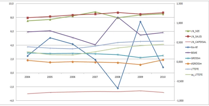
Figure 1 - Dependent Variables

This graph represents the behaviour of the dependent variables trough the period from 2004 to 2010. The left

axis represents the scale for the LN_SIZE, LN_SALES and LN_CAPEXSAL. The right axis represents the scale

for: Rm_Rf, BEME, GROSSm, dGROSSm, LTTDTE, and sq_LTTDTE.

The above figure describes the behaviour of the average of the dependant and independent

variables during the period studied. The analysis of the graph does not reveal the presence of

a defined trend. Also each variable reveals different behaviours, which suggests that the

regression should not be affected by spurious relations between the dependent and

independent variables.

We begin by constructing a pooled OLS with robust standard errors that fit the model

(27)

20

Table 3 - Model 1: Pooled OLS

This tables present the results for a Pooled OLS model with robust standard errors using 280 observations, covering a period of 7 years, from 2004 to 2010. The data was organized as panel data. We included results for the coefficients, standard errors, t-ratios, and p-values. We added a significance column which contains a * if the variable is significant at 10% level, ** if the variable is significant at a 5% level, and *** if the variable is significant at 1% level. We also add an extra table to include the usual fitness tests.

Model 1: Pooled OLS, using 280 observations Included 40 cross-sectional units

Time-series length = 7 Dependent variable: Rpt_Rft Robust (HAC) standard errors

Coefficient Std. Error t-ratio p-value Significance

Const 0.272982 0.291178 0.9375 0.34934

Rmt_Rft 0.712783 0.0685166 10.4031 <0.00001 ***

BEMEpt -0.237037 0.0751349 -3.1548 0.00179 ***

LN_SIZEpt 0.0558484 0.0667907 0.8362 0.40380

GROSSpt -0.0348769 0.279846 -0.1246 0.90091

dGROSSpt 1.09242 0.601212 1.8170 0.07032 *

LTDTTEpt 0.289007 0.142789 2.0240 0.04396 **

sq_LTDTTEpt -0.18499 0.0669499 -2.7631 0.00612 ***

LN_CAPEXSALpt -0.0434963 0.0394642 -1.1022 0.27137

LN_SALESpt -0.0714164 0.0551825 -1.2942 0.19671

CRISIS -0.0666823 0.0594241 -1.1221 0.26280

Mean dependent var 0.254708 S.D. dependent var 0.642641

Sum squared resid 65.06652 S.E. of regression 0.491816

R-squared 0.435301 Adjusted R-squared 0.414309

F(10, 269) 20.73600 P-value(F) 2.28e-28

Log-likelihood -192.9897 Akaike criterion 407.9793

Schwarz criterion 447.9620 Hannan-Quinn 424.0164

rho -0.087654 Durbin-Watson 1.950140

The model suggests that only Rmt −Rft, BEMEpt, dGROSSpt, LTDTTEpt and

pt

LTDTTE

sq_ are statistically significant variables.

From the results obtained we can conclude that as expected the market is positively

correlated with Stock returns. High BE/ME ratios have a negative impact on returns, and in

this case SIZE has no statistical significant impact on stock returns. The results also allow us

to conclude that improvements in Gross Margin have a positive effect on stock returns,

which reinforces our view that an improvement in Low Costs Achieved CA is important in

(28)

21

an increment in long term debt is positive on returns, but as debt starts to accumulate this

effect starts to be marginally negative.

This model has a 43.53% R-squared, which is high.

However after performing the Breusch-Pagan test, detailed in Annex 2, with a 0.03 p-value,

reveals that a GLS model with random effects is preferable to the pooled OLS.

This way we computed a GLS with random effects model, which obtained the following

results:

Table 4 - Model 2: Random Effects GLS

This table presents the results for a random effects GLS model using 280 observations and covering a period of 7 years, from 2004 to 2010. The data was organized as panel data. We included results for the coefficients, standard errors, t-ratios, and p-values. We added a significance column which contains a * if the variable is significant at 10% level, ** if the variable is significant at a 5% level, and *** if the variable is significant at 1% level. We also add an extra table to include the usual fitness tests. The present model is preferable to the model in table 3 as suggested in the tests in annex.

Model 2: Random-effects (GLS), using 280 observations Included 40 cross-sectional units

Time-series length = 7 Dependent variable: Rpt_Rft

Const 0.272982 0.328581 0.8308 0.40683

Rmt_Rft 0.712783 0.0651397 10.9424 <0.00001 ***

BEMEpt -0.237037 0.10058 -2.3567 0.01916 **

LN_SIZEpt 0.0558484 0.0615369 0.9076 0.36492

GROSSpt -0.0348769 0.371981 -0.0938 0.92537

dGROSSpt 1.09242 0.499181 2.1884 0.02950 **

LTDTTEpt 0.289007 0.217886 1.3264 0.18583

sq_LTDTTEpt -0.18499 0.136672 -1.3535 0.17702

LN_CAPEXSALpt -0.0434963 0.0443589 -0.9806 0.32769

LN_SALESpt -0.0714164 0.0566653 -1.2603 0.20865

CRISIS -0.0666823 0.0695061 -0.9594 0.33823

(29)

22

After performing the Hausman test (Annex 3), with a p-value of 0.135, we do not reject the

hypothesis that the GLS is consistent and therefore this model is preferable to the pooled

OLS shown before.

The results obtained from this model go in the same direction as the pooled OLS, with the

exception of the variables LTDTTE_pt and sq_LTDTTE_pt that are no longer significant.

The variable BEMEpt has a negative coefficient. This indicate that value or distressed stocks

have poor performance in this industry. This might happen as a consequence of persistent

weak earnings that are characteristic of companies with high BE/ME ratios (Fama and

French, 1993). The market may interpret historical bad earnings has management inability to

improve the company’s competitive position. The market (the coefficient of Rmt −Rft) has

a positive impact on stock returns as was expected in CAPM theory. The first difference of

gross margin, dGROSSpt, has a positive impact on returns, however GROSSpt is not

statistically relevant. Our interpretation is that investors already discounted the ability of a

company to achieve a determined GROSSpt, what the market wants to know is the capacity

to improve the efficiency of the company. Therefore the market, in average, will reward any

improvement, or punish any fallback in the operations efficiency without caring about the

starting point.

Additionally we must note that in neither model we found the variable CRISIS relevant.

However, we think that this happens because the R_mt −R_ft already captures the negative

effects of the crisis in the market. So although the crisis appears to have no impact on our

model it would be interesting to construct two models for the same observations, one before

and other during the Subprime crisis.

We started by constructing a model restricted to CRISIS = 0 (before the subprime crisis) and

we have followed the same procedure as before. We started by constructing a pooled OLS

with Robust Standard Errors (Annex 4), and then after performing the Hausman test which

resulted in a 0.002 p-value (Annex 5), we decided to that a GLS with Fixed Effects was a

(30)

23

Table 5 - Model 3: Fixed-Effects GLS Before Crisis

This table presents the results for a fixed-effects GLS model using 160 observations and covering a period of 4 years, from 2004 to 2007. The data was organized as panel data. We included results for the coefficients, standard errors, t-ratios, and p-values. We added a significance column which contains a * if the variable is significant at 10% level, ** if the variable is significant at a 5% level, and *** if the variable is significant at 1% level. We also add an extra table to include the usual fitness tests. We chose to construct this model to be able to extract the impact of the CA in the stock returns before the subprime crisis of 2008.

Model 3: Fixed-effects, using 160 observations Included 40 cross-sectional units

Const -2.78514 1.8335 -1.5190 0.13160

Rmt_Rft 0.881271 0.209493 4.2067 0.00005 ***

BEMEpt -1.0802 0.295165 -3.6597 0.00039 ***

LN_SIZEpt -0.296697 0.193251 -1.5353 0.12756

GROSSpt -1.44819 1.13689 -1.2738 0.20539

dGROSSpt 4.62935 1.06773 4.3357 0.00003 ***

LTDTTEpt 0.752235 0.727596 1.0339 0.30345

sq_LTDTTEpt -0.446638 0.523684 -0.8529 0.39556

LN_CAPEXSALpt -0.143176 0.106756 -1.3412 0.18261

LN_SALESpt 0.69351 0.343325 2.0200 0.04579 **

F(48, 111) 1.639281 P-value(F) 0.017565

This regression provides interesting results. First the signal of the significant variables stays

the same as before, but now the natural log of Sales, LN_SALES_pt, is also significant. The

fact that Sales have a positive impact on stock returns suggests the presence of Economies of

Scale as a CA, before the crisis. This makes theoretical sense. As we said before the Steel

Industry has enormous fixed costs, which causes the Steel Mills to operate as near as possible

to its total capacity. So before the crisis started there was a level of demand that allowed the

mills to pursue Economies of Scale in order to obtain CA. This way, as we observe in the

(31)

24

returns. However the crisis brought lower demand, but at the same time the fixed costs

remained the same, which usually means losses to the Steel producers. Therefore, during a

crisis, a Steel producer is not able to pursue economies of scale. The mills usually change the

focus to streamlining the operations.

We should also add that in this regression the coefficient of GROSS_pt is even bigger, which

suggests that the market puts even larger pressure on the ability of a company to be efficient.

Now we should compare these results with a regression during the crisis, CRISIS = 1.

Again we started with a pooled OLS with robust standard errors, which this time, after

reviewing the tests, in Annex 6, the pooled OLS is the preferable model. The joint

significance test yielded a p-value of 0.68, which means that the pooled OLS should not be

rejected in favour of a GLS with fixed effects and the Breusch-Pagan test yielded a p-value of

0.26, which means that we should not reject the pooled OLS in favour of a GLS with random

effects.

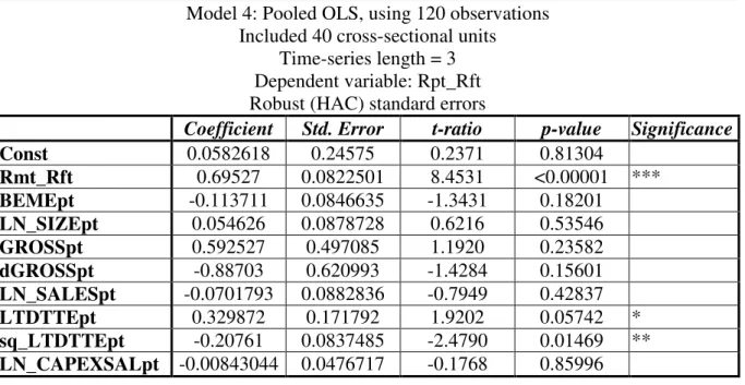
Table 6 - Model 4: Pooled OLS During Crisis

This table presents the results for a pooled OLS model with robust standard errors using 120 observations and covering a period of 3 years, from 2008 to 2010. The data was organized as panel data. We included results for the coefficients, standard errors, t-ratios, and p-values. We added a significance column which contains a * if the variable is significant at 10% level, ** if the variable is significant at a 5% level, and *** if the variable is significant at 1% level. We also add an extra table to include the usual fitness tests. We chose to construct this model to be able to extract the impact of the CA in the stock returns during the subprime crisis that started in 2008.

Model 4: Pooled OLS, using 120 observations Included 40 cross-sectional units

Const 0.0582618 0.24575 0.2371 0.81304

Rmt_Rft 0.69527 0.0822501 8.4531 <0.00001 ***

BEMEpt -0.113711 0.0846635 -1.3431 0.18201

LN_SIZEpt 0.054626 0.0878728 0.6216 0.53546

GROSSpt 0.592527 0.497085 1.1920 0.23582

dGROSSpt -0.88703 0.620993 -1.4284 0.15601

LN_SALESpt -0.0701793 0.0882836 -0.7949 0.42837

LTDTTEpt 0.329872 0.171792 1.9202 0.05742 *

sq_LTDTTEpt -0.20761 0.0837485 -2.4790 0.01469 **

(32)

25

F(9, 110) 22.95393 P-value(F) 1.59e-21

The set of results provide us again with interesting results. The variables dGROSSpt and

LN_SALESpt are no longer significant. On the other hand, the two proxies for Financial

Strenght and Financial Skills, LTDTTEpt and sq_LTDTTEpt are now relevant. We can

speculate that during the crisis the investors are less worried with the operational excellence

of a steel mill, and more worried about its chance of survival, than in bad times. During a

crisis the survival of a Steel producer is more dependent on the ability to manage debt. This

means that the financial ability and strength is a major CA in the Steel industry during an

economic crisis.

We think the results are clarifying in relation to the importance of CAs to stock returns. Not

all of the CAs we tested were considered relevant, but we have seen that the importance of

the competitive advantages also depends on the external competitive scenario where the

company operates.

6 – Limitations and Problems

In this section we would like to emphasize the limitations in this work.

First of all we must alert to the fact that every limitation known to the models used in this

work are also present here.

In every work the foundations of the conclusions are based on assumptions. If the

assumptions hold, the conclusions obtained are good, if not, then the conclusions will be

undermined. We are not an exception to this rule. In section 3 we defined assumptions

relative to the variables to be used as proxies for CAs. We have justified our choices with

robust arguments, however there is always the possibility of our proxies not being the most

(33)

26

The information disclosed by public companies is also, in many cases, insufficient to extract

quantifiable variables that are useful to create proxies for CAs. Accounting measures and

other loopholes might constitute too much noise for some proxies to be useful.

The lack of literature and models already testing the relation between CAs and stock returns

is also a limitation since we had to create our own framework, and it has not been tested

before in the same context.

In synthesis our work has some degree of limitations, but nevertheless we incurred in a big

effort to fundament our work with the best literature available and statistical models

(34)

27

7 – Conclusions and Insights for Future Research

In the light of the results obtained we can conclude that Competitive Advantages (CAs)

cannot be rejected as sources of excess stock returns. The main model, including pre and after

crisis data, revealed that an improvement in Low Costs Achieved do have a relevant impact

on the returns of the companies studied, after controlling for Fama-French variables. This is

in accordance with the strategy literature, Porter (1985), which states that CAs should lead to

higher than average profits, and with valuation theory, Williams (1938), which states that

above average returns profits should lead to above average investment returns.

In the case of the pre-crisis model, the results indicate again that an improvement of Low

Costs Achieved cannot be rejected as source of excess returns. This model also indicates that

Economies of Scale are source of excess returns. We can conclude that under stability the

market simply rewards improvements in operational efficiency and scale (which is related

with operational efficiency). This is a coherent result since Steel mills operations have to

absorb the huge fixed costs incurred by the mills (Thompson, 1992). Better than average

operations efficiency will result in better than average returns.

However the post-crisis model suggests that only Financial Skills and Financial Strength CA

is source of excess returns. This means that in uncertainty contexts, the market does not care

about operational efficiency anymore, focusing on closely monitoring the financial health of

the company. With the economic down cycle, the market recognizes that the Steel mills will

no longer be efficient. So the investors prefer to focus on the company’s ability to survive

during bad times.

This findings brings a new light to the process of assessing perspectives for any given

company. If the security analyst selects the appropriate CAs useful in a given industry, and is

able to do a quantitative study, then he might, with more ease, find the companies that will

have more probability and perform better. This might be useful in the choice of assumptions

for the valuation matrix, conferring added robustness to the valuation.

This study should be made for other industries, and for other CAs, in order to provide more

information. Works in other sectors might be done to help sustaining or to refute our theory.

Also studies about the robustness of the proxies used might be done to help sustain or refute

(35)

28

References

Banz, R. W. (1981), “The Relationship between Return and Market Value of Common

Stocks,” Journal of Financial Economics, nº 9 (1981), pp. 3-18;

Barney, Jay B. (1986), “Strategic Factor Markets: Expectations, Luck, and Business

Strategy,” Management Science, Vol. 32, No. 10, Oct. 1986, pp. 1231-1241;

Basu, S. (1983), “The Relationship between Earnings Yield, Market Value, and Return for

NYSE Common Stocks: Further Evidence,” Journal of Financial Economics, nº 43 (1983),

pp. 129-156;

Bhandari, L. C. (1988), “Debt/Equity Ratio and Expected Common Stock Returns: Empirical

Evidence,” Journal of Finance, nº 43 (1988), pp. 507-528;

Black, Fischer (1972), “Capital Market Equilibrium with Restricted Borrowing,” Journal of

Business, nº 45, pp. 444-455.

Carroll, Peter, (1982), “The Link Between Performance and Strategy,” The Journal of

Business Strategy, Vol. 2, No 4, pp. 3-20;

Christensen, Clayton M. (2001), “The Past and Future of Competitive Advantage,” MIT

Sloan Management Review, Winter 2001, pp 105-109;

Chugh, Lal C. and Joseph W. Meador, (1984), “The Stock Valuation Process: The Analysts’

View,” Financial Analysts Journal, November-December, 1984, pp.41-48;

Cottle, Sidney, Roger Murray and Frank Block (1988), “Securities Analysis,” 5th Edition,

McGraw-Hill Professional;

Daniel, Kent and Sheridan Titman (1997), “Evidence on the Charateristics of Cross Sectional

Variation in Stock Returns,” The Journal of Finance, Vol. 52, Nº 1 (March, 1997), pp.1-33;

Day, George S. and Robin Wensley (1988), “Assessing Advantage: A Framework for

(36)

29

Drucker, Peter F. (1998); “The Discipline of Innovation”; Harvard Business Review

November-December 1998;

Fama, Eugene F. (1970), “Efficient Capital Markets: A Review of Theory and Empirical

Work,” The Journal of Finance, Vol. 25, No. 2, pp. 383-417;

Fama, Eugene F. and Kenneth R. French (1992), “The Cross-Section of Expected Stock

Returns, The Journal of Finance, Volume 47, Issue 2 (June, 1992),427-465;

Fama, Eugene F. and Kenneth R. French (1993), “Common Risk Factors in Returns on

Stocks and Bonds,” Journal of Financial Economics, nº 3, pp. 3-56;

Fama, Eugene F. and Kenneth R. French (1995), “Size and Book-to-Market Factors in

Earnings and Returns,” The Journal of Finance, Vol. L, Nº1, March 1995, pp. 131-155;

Fisher, Philip A. (1958), Common Stocks and Uncommon Profits, Harper& Brothers, 1958;

Hofer, C. and D. Schendel, (1978), Strategy Formulation: Analytical Concepts, St Paul, MN:

West;

Hurley, Robert F. And G. Thomas M. Hult (1998), “Market Orientation, and Organizational

Learning: An Integration and Empirical Examination,” The Journal of Marketing, Vol. 62,

No. 3 (Jul., 1998), pp. 42-54;

Ireland, R. Duane, Robert E. Hoskisson, Michael A. Hitt (2007), “The Management of

Strategy: Concepts and Cases,” 8th Edition, South-Western Cengage Learning;

Keynes, John Maynard (1935), “The General Theory of Employment, Interest and Money,”

Classic Books America (2009);

Lakonishok, Josef, Andrei Shleifer, and Robert W. Vishny, (1994), “Contrarian Investment,

Extrapolation and Risk,” Journal of Finance,Nº49, pp. 1541-1578;

Lintner, John, (1965), “The Valuation of Risk Assets and the Selection of Risky Investment

in Stock Portfolios and Capital Budgets,” Review of Economics and Statistics, nº 47, pp.

(37)

30

MaConaugby, Daniel L., Charles H. Matthews and Anne S. Fialko (2001), “Founding Family

Controled Firms: Performance, Risk and Value, Journal of Small Business Management, Vol.

39, Issue 1, pp. 31-49, January 2001;

Markowitz, Harry (1959), Portfolio Selection: Efficient Diversification of Investments

(Wiley, New York).

Markowitz, Harry M. (1952), “Portfolio Selection,” The Journal of Finance, Vol. 7, No. 1,

March 1952, pp. 77-91;

Myers, S. C. and R. A. Brealey, 2003, Principles of Corporate Finance, Boston:

McGrawHill;

Porter, Michael E. (1985); “Competitive Advantage”; New York: The Free Press;

Reichstein, Toke and Ammon Salter (2006), “Investigating the sources of process Innovation

among UK manufacturing firms,” Industrial and Corporate Change, pp. 1-30, July 2006;

Rugman, Alan M. and Alain Verbeke (2008), “Internalization theory and its impact on the

field of international business,” Jean J. Boddewyn (ed.) International Business Scholarship:

AIB Fellows on the First 50 Years and Beyond (Research in Global Strategic Management,

Volume 14), Emerald Group Publishing Limited, pp.155-174;

Sharpe, William F. (1964), “Capital Asset Prices: a Theory of Market Equilibrium under

Conditions of Risk,” Journal of Finance, nº 19, pp. 425-442.

Thompson, Arthur A., A. J. Strickland (1992), “Cases in Strategic Management,” 4th Edition,

Irwin, 1992;

Thompson, Victor A. (1965); “Bureaucracy and Innovation”; Administrative Science

Quarterly, Vol. 10, No. 1, Special Issue on Professionals in Organizations (Jun., 1965), pp.

1-20;

Tobin, James (1958), “Liquidity Preference as Behaviour Towards Risk,” The Review of

(38)

31

Vaihekoski, Mika (2009), “Pricing of Liquidity Risk: Empirical Evidence from Finland,”

Applied Financial Economics, Volume 19, Issue 19, 2009, pp.1547-1557;

Veríssimo, José M. (2004), Hard-to-Copy Services: Research Into the Factors That Make

Successful Service Products Difficult to Imitate, PhD Thesis, Manchester Business School;

INSTITUTO SUPERIOR DE ECONOMIA E GESTÃO

UNIVERSIDADE TÉCNICA DE LISBOA