M ESTRADO A CTUARIALS CIENCE T RABALHOF

(1)

M

ESTRADO

A

CTUARIAL

S

CIENCE

T

RABALHO

F

INAL DE

M

ESTRADO

DISSERTAÇÃO

MODELING SOVEREIGN DEBT WITH LÉVY PROCESSES

GONÇALO ANDRÉ NUNES PEREIRA

(2)

M

ESTRADO EM

A

CTUARIAL

S

CIENCE

T

RABALHO

F

INAL DE

M

ESTRADO

DISSERTAÇÃO

MODELING SOVEREIGN DEBT WITH LÉVY PROCESSES

GONÇALO ANDRÉ NUNES PEREIRA

O

RIENTAÇÃO

:

R

AQUEL

G

ASPAR

J

OÃO

G

UERRA

(3)

Abstract

We propose to model the sovereign credit risk of five Euro area countries (Portu-gal, Ireland, Italy, Greece and Spain) under a first passage structural approach, replacing the classical geometric Brownian motion dynamics with a pure jump L´evy process. This framework caters for skewness, fat tails and instantaneous defaults, thus addressing some of the main drawbacks of the Black-Scholes model. We compute the survival probability as the price of a discrete barrier option, using an option pricing method based on the approximation of the transition density as a Fourier-cosine series expansion. Assuming a deterministic recovery rate, we calibrate the Carr–Geman–Madan–Yor (CGMY) L´evy model to weekly Credit Default Swaps data and obtain the default probability term structure. By drawing on the representation of the Variance Gamma process (a particular instance of the CGMY model) as a time-changed Brownian motion, we accom-modate dependency between sovereigns via a common time change. We then illustrate a possible multivariate calibration procedure and simulate the joint default distribution.

(4)

Resumo

Propomos modelizar o risco de crédito soberano de cinco pa´ıses da zona Euro (Portugal, Irlanda, Itália, Grécia e Espanha) seguindo uma abordagem estrutural de primeira passagem em que o movimento Browniano geométrico é substitu´ıdo por um processo de Lévy regido apenas por uma componente de saltos. Deste modo, introduzimos incrementos assimétricos e leptocúrticos e a possibilidade de incumprimento instantâneo, removendo assim algumas das principais limita¸cões do modelo Black-Scholes.

Calculamos a probabilidade de sobrevivência como pre¸co de uma op¸cão bar-reira discreta, utilizando um método de valoriza¸cão de op¸cões baseado na aproxi-ma¸cão da densidade de transi¸cão como expansão em série de Fourier de cossenos. Assumindo uma taxa de recupera¸cão determin´ıstica, calibramos o modelo de Lévy Carr–Geman–Madan–Yor (CGMY) utilizando spreads de Credit Default Swaps semanais e obtemos a estrutura temporal de probabilidades de incumpri-mento. Tiramos ainda partido da representa¸cão do processo Variance Gamma (uma instância do modelo CGMY) como movimento Browniano modificado tem-poralmente para considerar uma estrutura de dependência entre os riscos de crédito soberanos através de uma modifica¸cão temporal comum. Em seguida, ilustramos um poss´ıvel procedimento de calibra¸cão multidimensional e obtemos a distribui¸cão de sobrevivência conjunta via simula¸cão.

(5)

Acknowledgments

I thank my supervisors, Jo˜ao Guerra and Raquel Gaspar, their welcoming, support and commitment.

(6)

List of Figures

4.1 Daily mid-quotes for Portuguese and Irish CDS spreads . . . 24

4.2 Daily mid-quotes for Italian and Spanish CDS spreads . . . 25

4.3 Daily mid-quotes for Greek CDS spreads . . . 25

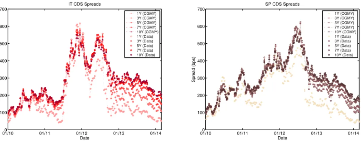
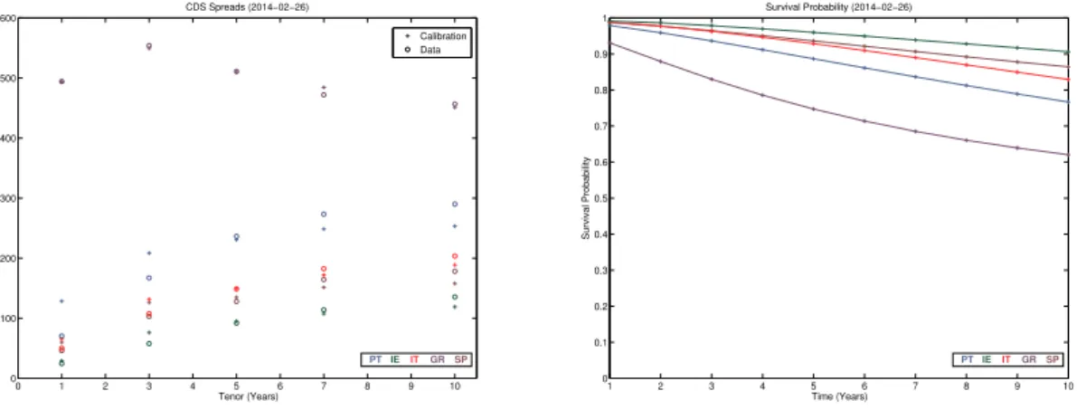
5.1 Calibration of the CGMY model: Portugal and Ireland . . . 26

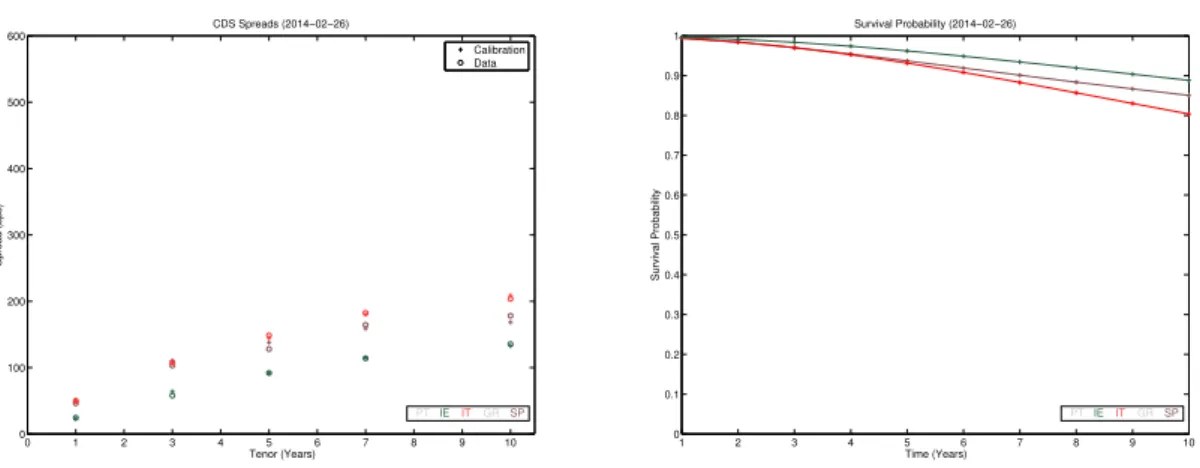
5.2 Calibration of the CGMY model: Italy and Spain . . . 27

5.3 Calibration of the CGMY model: Greece . . . 27

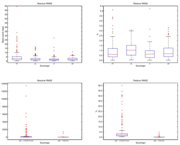
5.4 Calibration of the CGMY model: absolute and relative RMSE . . . 28

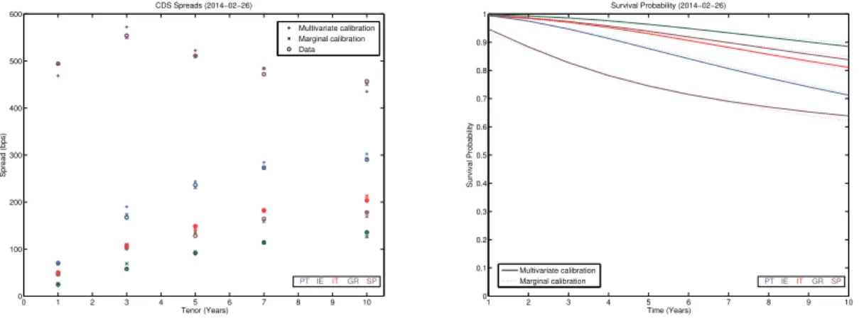
6.1 Joint calibration of the multivariate VG model with a common time change for all sovereigns . . . 31

6.2 Joint calibration of the multivariate VG model with a common time change for Ireland, Italy and Spain . . . 32

6.3 Joint calibration of the multivariate VG model with a common time change component for all sovereigns and an idiosyncratic time change component for Portugal and Greece . . . 33

6.4 Joint simulation of paths under the multivariate VG model . . . 34

B.1 Evolution of the calibrated CGMY parameters over time: Portugal . . . 41

B.2 Evolution of the calibrated CGMY parameters over time: Ireland . . . 42

B.3 Evolution of the calibrated CGMY parameters over time: Italy . . . 43

B.4 Evolution of the calibrated CGMY parameters over time: Spain . . . 43

B.5 Evolution of the calibrated CGMY parameters over time: Greece . . . 44

B.6 Default probability term structure: Portugal and Ireland . . . 45

B.7 Default probability term structure: Italy and Spain . . . 45

B.8 Default probability term structure: Greece . . . 45

B.9 Calibration of the CGMY model vs. calibration of the geometric Brownian motion model . . . 46

(9)

List of Tables

2.1 The CGMY model parameter Y . . . 13

3.1 Discretization parameters for the COS method . . . 22

3.2 2012–2013 Euro area default events . . . 23

B.1 CGMY calibration: descriptive statistics of the RMSE distribution . . . 44

B.2 Calibration of the CGMY model vs. calibration of the geometric Brownian motion model . . . 46

B.3 Comparison between exponential CGMY and geometric Brownian motion dy-namics . . . 47

B.4 Calibration of the multivariate VG model . . . 48

B.5 Joint default probabilities under the multivariate VG model . . . 49

(10)

Chapter 1

Introduction

The classical structural approach to corporate credit risk modeling describes the asset value process as a geometric Brownian motion and defines default either as the equity value drop-ping to zero at maturity (Merton 1974) or as the first passage time of an exogenous default barrier (Black and Cox 1976). It establishes an intuitive relationship between default and the value of a firm’s assets, and its dynamics allows the straightforward computation of survival probabilities and the credit spread term structure. However, it is known that the Black-Scholes framework used is unable to capture several well-grounded empirical evidences, such as the skewed and leptokurtic distribution of returns. These shortcomings are rooted in the assumption of Gaussian increments, that imply continuous sample paths. We can overcome them by extending the modeling dynamics to the wider class of L´evy processes. In particu-lar, we can then capture sudden shocks through the introduction of jumps in the asset value process, thereby removing the local predictability of default.

The link between asset value and default is lost when we move from the corporate to the sovereign credit risk realm. Indeed, the estimation of a sovereign asset value process from sound economic fundamentals is still very much an open problem. Additionally, sovereign default can be triggered from strategical political decisions. If a government manages to bridge the gap between the burden of defaulting (such as raising future borrowing costs or facing trade sanctions) and its benefits (immediate debt relief through renegotiation of the original issuance terms), it might find a proper incentive to formally declare default.

In this work, we have not endeavored to address the problem of defining and estimating a suitable sovereign value process. Instead, we co-opt the notion of corporate asset value process and assume that the market price of sovereign default, as measured by the Credit Default Swaps (CDS) spreads term structure,implicitly incorporates information on alatent

sovereign value process. We recognize that the rationale behind this assumption is weaker than the one we could presumably reach had we attempted to devise an explicit sovereign value model. However, as our results will show, this simplified framework will allow us to accurately reproduce the CDS market data both under regular and distress circumstances. We believe this fact upholds our modeling approach.

(11)

2

modeling the latent sovereign value process.

The COS method approximates the transition density as a Fourier-cosine series expan-sion, obtainable from the process characteristic function. It requires only the analytical knowledge of the latter and so provides a tractable and flexible way to compute the survival probability and calibrate L´evy models from CDS market data.

Our main objective is the univariate calibration of the CGMY model and the computation of the implied default probability term structure, spanning the period from January 2010 to the end of February 2014. A secondary goal is the introduction of dependency between the underlying sovereign value processes using the subclass of L´evy processes representable as a time-changed Brownian motion. To this effect, we consider a common time change compo-nent. The univariate calibration procedure can be easily adapted to the multidimensional structure, and joint and conditional survival probabilities estimated via simulation.

We believe our work makes three relevant empirical contributions. First, even though we make a strong (and, in a sense, exogenous) assumption on the modeling dynamics, it shows that the CGMY model accurately captures the features of the CDS term structure. The fact that we have used an extensive dataset spanning the main stages of the Euro area sovereign debt crisis further supports the quality of the fit and the model’s flexibility. In particular, the calibration has successfully captured extreme behavior under severe distress periods, such as high peaks and inversion effects on the CDS spreads term structure. Secondly, our results provide evidence illuminating the relationship between the data lifecycle and the process structure: namely, a clear switch from an infinite to a finite activity regime under distress. Finally, we provide an extension to a multidimensional setting, incorporating dependency, and illustrate how it can be used to obtain the joint default distribution.

(12)

Chapter 2

Structural credit risk modeling

under L´

evy dynamics

2.1 The structural approach

Under the structural approach to corporate credit risk modeling, debt and equity are treated as contingent claims on a firm’s asset value process.

2.1.1 The classical Merton approach

In Merton’s model (1974), the firm defaults on its debt if the value of the equity drops to zero at the debt’s maturity T.1 The firm’s asset value processVt is modeled as a geometric Brownian motion,

dVt=µVtdt+σVtdBt, V0 >0⇒Vt=V0exp

µ₋ 1

2σ

2

t+σBt

,

whereµ is the drift parameter,σ is the volatility and Bt is a standard Brownian.

As the increments of a Brownian motion are normally distributed, the computation of the default probabilities is straightforward:

Pdef(T) = Φ





ln_VK₀− µ₋1₂σ2T σ√T



,

whereK denotes the notional value of the debt.

Merton’s model treats equity as a European call option on the value of the firm held by the shareholders, with strike price equal to the outstanding notional value of debt.2 _This

leads to Black-Scholes-type formulæ to value the equity and price defaultable bonds. The limitations of this approach are clear: default can only occur at the debt’s maturity

T, and the firm value can be arbitrarily close to zero without triggering default.

2.1.2 The first passage approach

Black and Cox’s model (1976) overcomes these limitations by introducing an exogenous default barrier D, following the empirical evidence of default events occurring before the equity drops to zero. Default is redefined as the first time the value process Vt hits this barrier. Under the geometric Brownian motion dynamics for Vt, default probabilities are

(13)

2.1 The structural approach 4

also easily obtainable, as the distribution of the running minimum of a Brownian motion with drift,

min

s≤t{µs+σBs},

is known to be Inverse Gaussian. This leads to the following default probability formula (Lando 2004, 259-260):

Pdef(t) = Φ





ln_VD

0

− µ₋1₂σ2t σ√t



+

D V0

2(µ−

1 2σ2)

σ2 Φ





ln_VD

0

+ µ₋1₂σ2t

σ√t



.

We can describe the survival probability as the price of a barrier option without discount-ing. As a consequence, Black and Cox’s model is a natural framework for the application of option pricing techniques.

2.1.3 Drawbacks and desirable properties

The structural approach is conceptually attractive by providing a clear link between default and the firm’s asset value process. However,under the Brownian motion dynamics default is

locally predictable, leading to inconsistencies with intuition and empirical observation. The

most striking of these is the unrealistic behavior of the short-term end of the credit spread3 term structure, which will always approach zero.

A realistic credit risk model should first and foremost treat default times as locally

un-predictable, which would suggest modeling the firm’s asset value using a process with jumps.

These could reflect the arrival of new information leading to sudden shocks in the asset value, a behavior that processes with continuous sample paths, such as the Brownian motion, can not capture. Proceeding this way, we would be introducing a mechanism of instantaneous default, thus avoiding artificial techniques to build it into the model such as, for example, making the default threshold barrier stochastic.

In addition, empirical evidence from stock returns suggests that any process describing the firm’s asset value should produce a returns distribution withskewness and positive excess

kurtosis (fat-tail behavior). This is not consistent with the Gaussian framework of the

Black-Scholes model.

L´evy processes, introduced in the next section, provide distributions with these charac-teristics.

2.1.4 Modeling sovereign debt

We have been describing the structural approach framework under a classical corporate credit risk setting. However, when applying such framework to the problem of modeling sovereign credit risk, we can not interpret Vt as an asset value process in a strict sense, nor can we easily define the default barrier in terms of the outstanding value of debt. This is the main reason why the structural approach is a less trodden path in sovereign credit risk modeling. A first strand of the literature attempts to define and estimate the sovereign value (or a suitable proxy). Karmann and Maltritz (2003) and Clark and Kassimatis (2004) use the present value of net exports as a measure of a sovereign’s market value. This approach might suit developing countries, but it falls short of capturing the sovereign value in advanced economies or countries within a monetary union. Currie and Velandia (2002) produce a stylized government balance sheet: assets are the discounted values of fiscal revenues, for-eign reserves and marketable securities; liabilities are the discounted values of government

(14)

2.2 Financial modeling with L´evy processes 5

spending, public debt and contingent liabilities (such as government guarantees, bailouts or deposit insurance schemes). The latter are especially difficult to estimate, as they are linked with the financial performance of the private sector, but the model as a whole is prone to strong forecasting assumptions.

Another strand of the literature discards the direct estimation of the sovereign value and introduces exogenous default indicator processes. Hui and Lo (2002) resort to the foreign exchange rate; Moreira and Rocha (2004) develop accounting ratios involving macro-financial variables. Oshiro and Saruwatari (2005) employ stock indexes as a measure of sovereign “equity” under a classical Black-Scholes structural approach.

A sovereign default event can take several forms: non-payment of principal or interest due, a debt exchange (for claims of lower value), a moratorium or an official repudiation of debt. In contrast to the corporate case, a government might find incentives to default on economic reasons other than the strict ability-to-pay argument that compares the asset value to the outstanding notional of the debt. Strategic political concerns will also play a major role, namely the reputational effect on future borrowing costs and a possible decrease in economic output due to trade sanctions. Along these lines, the default indicator process could reflect the difference between the costs and benefits of default (Eaton and Gersovitz, 1981; Calvo, 1988).

When setting the scope of the current work, we have pragmatically decided not to address the direct estimation of a sovereign value process and focus mainly on the benefits of replac-ing the geometric Brownian motion dynamics with a suitable L´evy process. As previously mentioned, we will work under the assumption thatVtrepresents an unobservable sovereign value process, that implicitly determines the CDS spreads term structure and so acts as a default indicator. The default barrier will be redefined in terms of an assumed recovery rate given default and the initial value of the process. Chapter 3 will detail this procedure. In the next section, we address the problem of introducing a suitable L´evy dynamics to model the latent value processVt.

2.2 Financial modeling with L´

evy processes

2.2.1 A brief historical background

L´evy processes have been successfully used in asset pricing models to address some of the main limitations of the Brownian motion dynamics, such as the inability to account for the negative skewed and leptokurtic distribution of log-returns, or the volatility smile4. They are a natural generalization of the Brownian motion model, keeping the independence and stationarity of increments, but crucially introducing jumps. These can capture real price dis-continuity phenomena and incorporate sudden, unexpected information shocks. In addition, they account for skewness and fat tails.

The non-normality of stock returns was a well established empirical fact as early as 1963, when Maldelbrodt proposed theα-stable class of distributions for stock prices (Mandelbrodt 1963). The Normal distribution is obtained with α = 2 and the Cauchy distribution with

α = 1. When α < 2, the density is more peaked around the center than the Gaussian distribution and the variance is infinite, implying fat tails. When α_≤1 the expected value does not exist. The α-stable model is a L´evy model, but empirical evidence has rejected its adequacy to describe stock price returns.

One of the first attempts at introducing discontinuities in the asset price process was the jump-diffusion model of Merton, where a Compound Poisson process with Gaussian jumps

4_{The graphic representation of volatility against option strike prices, constant under the Black-Scholes}

(15)

is added to a diffusion (Merton 1976). We will briefly illustrate the properties of the jump-diffusion strand of models in Section 2.3, resorting to the Kou model (Kou 2002), where the jumps have a double exponential distribution.

Another strand of L´evy models relies on the Generalized Hyperbolic distribution, intro-duced by Barndorff-Nielsen (1977) to model the grain size of wind-blown sand. Two partic-ular models of this type are the exponential Hyperbolic motion (Eberlein and Keller 1995) an the exponential Normal Inverse Gaussian (Barndorff-Nielsen 1998). Both have proved capable of accurate fits to empirical stock prices log-returns. Eberlein and Prause (1998) provide a comprehensive account of the family of Generalized Hyperbolic L´evy processes.

The Normal Inverse Gaussian model is a pure jump model with infinite activity5 and finite variation. It dispenses with a diffusion component and so it has discontinuous sample paths. Local price uncertainty is captured not trough a constant volatility parameter but by the nature of the jumps, arising from pure supply and demand shocks.

More recent efforts have been focusing on the properties of infinite activity and infinite variation pure jump processes. The Variance Gamma model (Madan and Seneta 1990) was successfully used to describe Australian stock market data. The CGMY model (Carr et al.

2002) is an extension of the Variance Gamma model accounting for a finer structure of the very small jumps. Interestingly, the pure jump CGMY model has been shown to outperform a modified CGMY model with a diffusion component in describing equityindex data.6 We will use the CGMY dynamics to model the latent sovereign value process Vt and discuss its properties in Section 2.4.2. Even though the CGMY model does not present a tractable density function, its characteristic function has an analytic closed form representation. This makes the application of the Fast Fourier Transform (FFT) option pricing method feasible (Carr, Chang and Madan 1998). In fact, we will cast the survival probability problem as an option pricing problem in Chapter 3.

Yet another flavor of the use of L´evy processes in finance is the stochastic volatility model of Barndorff-Nielsen and Shephard (2001). It describes the volatility parameter as a station-ary Ornstein-Uhlenbeck process driven by non-Gaussian L´evy increments and addresses the problem of modeling the volatility smile.

An essential result for the multivariate default modeling technique we will develop in Chapter 6 is the representation of a semimartingale as a time-changed Brownian motion (TCBM) (Monroe 1978). In a TCBM, the deterministic time variable is replaced by an independent subordinator.7 _{If we take a L´evy subordinator, the TCBM construction will}

always lead to a L´evy process. This approach shifts the modeling focus to the time-change. The latter can be seen as a stochastic “clock”, reflecting the intensity of the economic activity (measured through the accumulated traded volume in the market) and the arrival of new pieces of information (Clark 1973, An´e and Geman, 2000).

Although it is a topic we do not address in this work, we should note that consider-ing independent increments might be too strong an assumption. The fractional Brownian motion model incorporates dependency of increments through a “long-range” dependency property. This means that the covariance between increments decays slowly to zero. How-ever, the application of the fractional Brownian motion to asset pricing problems might be problematic. In particular, the geometric fractional Brownian motion model allows arbitrage opportunities (Rogers 1997).

We now move to define L´evy processes and present some of their basic properties.

5_{As we will detail in the next section, this means that on every compact interval the process has a.s. an}

infinite number of jumps.

6_{The authors conjecture that possible diffusion components in individual prices are removed when indexes}

are considered.

(16)

2.2.2 Definition and characterization

We start by defining L´evy processes and will then present characterization results that will provide insight into their properties. We will also give some examples widely used in applica-tions to finance and motivate the choice of the CGMY model to describe the latent sovereign asset value (or default indicator) process, Vt.

Let (Ω,_F,Q) be a filtered probability space andL=_{Lt}_t_≥₀ a càdlàg8 process. Definition 2.1 (Lévy process). L such thatL₀ = 0 is a Lévy process if

• L has independent increments;

• L has stationary increments;

• L is stochastically continuous:

∀t>0, ε>0 lim

s→tPQ(|Lt−Ls|> ε) = 0.

Let ∆Lt:=Lt−Lt− be the jump size of the process at timet. The stochastic continuity

condition implies that the times where the jumps occur are random, i.e., we almost surely have ∆Lt= 0. In general, the number of jumps up to time t will not be bounded.

L´evy processes can be identified with the class of infinitely divisible distributions:

Proposition 2.1 (L´evy processes and infinitely divisible distributions). Let L be a L´evy

process. Lt has an infinitely divisible distribution9 and, conversely, if X is an infinitely

divisible distribution, there exists a L´evy process L such that L1=d X.

The proof can be found in Sato (1999) (Corollary 11.6).

We will describe a L´evy process using itscharacteristic function,

φLt(ω) :=E

eiωLt₌

Z

R

eiωxfLt(x)dx, (2.1) which is simply the Fourier transform of the density fLt(x). The characteristic function can be written as

φLt(ω) =e

tψ(ω)_,

whereψis a continuous function referred to as thecharacteristic exponent (Cont and Tankov 2004, Proposition 3.2). Working with the characteristic function is convenient for application purposes because, as we will see, it is easier to obtain analytic formulas for it than for the transition density.

The L´evy measure ν is defined as

ν(A) :=E[#_{t_∈[0,1] : ∆Lt∈A}], A∈ B(R),

and can be interpreted as the expected number of jumps of size in a given Borel set A, per time unit.

The following result is a central characterization of L´evy processes and provides the intuition underpinning their properties.

Theorem 2.1 (Lévy-Itô decomposition). Let L be a Lévy process and ν its corresponding Lévy measure. Then,

8_{Right-continuous with left limits.}

9_{A random variable}_X _{is infinitely divisible if for all}_n_∈_N_{there exist}_n _{i.i.d. random variables}_X(1/n)

j ,

(17)

• ν is a positive Radon measure on Rsuch that

ν({0}) = 0,

Z

|x|≤1

x2ν(dx)<_∞,

Z

|x|≥1

ν(dx)<_∞; (2.2)

• Lt can be decomposed in the following sum of independent components:

Lt=L(1)t +L

(2)

t +L

(3)

t ,

with

L(1)_t :=γt+σBt

L(2)_t :=

Z

|x|≥1, s∈[0,t]

xJX(ds×dx)

L(3)_t :=

Z

|x|<1, s∈[0,t]

x[JX(ds×dx)−ν(dx)ds],

where

JX([0, t]×A) = #{s∈[0, t] : ∆Ls∈A}

is a Poisson random measure counting the number of jumps in A up to t.

L(1)_t is a (continuous) Brownian motion with drift γ and volatilityσ. Furthermore, every continuous L´evy process is of this form. The second and third components, L(2)_t and L(3)_t , provide the jumps, as described by the L´evy measureν. L(2)_t is a compound Poisson process andL(3)_t is a square integrable martingale that can be seen as an infinite sum of compensated Poisson processes with jump sizes x.

As a corollary of the L´evy-Itˆo decomposition, we have the following decomposition of the characteristic function φLt(ω).

Theorem 2.2 (L´evy-Khintchine representation). The characteristic function of a L´evy pro-cess φLt(ω) has the following representation:

φLt(ω) =e

tψ(ω)_, where

ψ(ω) =iγω₋ σ 2_ω2

2 +

Z

R

eiωx₋1₋iωx1_|_x_|_<₁ν(dx)

is the characteristic exponent of L1, i.e., φL1(ω) =e

ψ(ω)_.

The triplet (γ, σ, ν) is called the L´evy triplet. γ _∈ R is the drift term, σ > 0 is the

diffusion coefficient and ν is a the L´evy measure, as previously defined.

Details on the previous two results can be found in Cont and Tankov (2004), Section 3.4. The characteristic exponent can be conveniently written as

ψ(ω) =ψ(1)(ω) +ψ(2)(ω) +ψ(3)(ω),

where

ψ(1)(ω) :=iγω₋σ 2_ω2

2

ψ(2)(ω) :=

Z

|x|≥1

eiωx₋1ν(dx)

ψ(3)(ω) :=

Z

|x|<1

eiωx₋1−iωxν(dx)

(18)

2.3 Jump-diffusion processes 9

2.2.3 The L´evy measure

The L´evy measure satisfies (2.2) and so it has no mass at the origin, its mass away from the origin is bounded and it can possibly have singularities around the origin. This means that in any compact interval a L´evy process may have infinitely many “small” jumps and at most a finite number of “large” jumps.

The L´evy measure also conveys information on the paths’ jumps and variation.

Proposition 2.2 (Lévy measure and the process activity). Let L be a Lévy process with Lévy triplet (γ, σ, ν).

• If ν(R)<_∞,L has finite activity, i.e., almost all paths have a finite number of jumps on any compact interval;

• If ν(R) = _∞, L has infinite activity, i.e., almost all paths have a infinite number of

jumps on any compact interval.

Intuitively, we can interpret the fluctuations in a infinite activity process modeling the value of a financial asset as arising from pure supply and demand shocks. In a finite activity process the shocks would be sudden and mostly exogenous, thus incorporating an unexpected arrival of information.

Proposition 2.3 (Lévy measure and the paths’ variation). Let L be a Lévy process with Lévy triplet (γ, σ, ν).

• If σ = 010 _and R

|x|≤1|x|ν(dx)<∞, almost all paths of L have finite variation;

• If σ ₆= 0 or R_|_x_|≤₁|x_|ν(dx) =∞, almost all paths of L have infinite variation.

The proofs of the two previous results can be found in Sato (1999) (Theorem 21.3 and 21.9, respectively). For a comprehensive review of the material in this section, with refer-ences to standard bibliography on L´evy processes and their application in finance, refer to Papapantoleon (2008).

Having introduced and provided characterization results for L´evy processes, we now move to present some examples relevant for the remainder of the work. Recalling that the key issue in credit risk modeling is how to obtain the survival probability, we observe that to compute it directly we would have to know the distribution of the process running minimum11_{, which will}

not be available in general. However, we will show in Chapter 3 that, by taking advantage of the representation of the characteristic function as a Fourier transform, we can use an efficient algorithm to numerically approximate the transition density (and from it the survival probability). This methodology will only require the knowledge of an analytic expression for the characteristic function.

2.3 Jump-diffusion processes

We have previously mentioned that the Merton jump-diffusion model was one of the first attempts to introduce discontinuities in the price process. Generally speaking, a jump-diffusion L´evy process merges adiffusion component with afinite activity jump process (i.e., a process such thatν(R)<_∞, by Proposition 2.2). Thereby, a jump-diffusion has the form

Lt=µt+σBt+ Nt

X

k=1 Jk,

10_{I.e., there is no Brownian component.}

(19)

2.4 Infinite activity, pure jumps processes 10

where the term µt+σBt, µ ∈ R, σ > 0, is a Brownian motion with drift, and the term

PNt

k=1Jk is a Compound Poisson process with intensity λ: Nt ∼ Poisson(λt) counts the number of jumps of Lt up to time t, and Jk i.i.d∼ J is the distribution of the (independent) jump sizes. Merton’s model assumes that J is normally distributed with mean µJ and varianceσ2_J, and we write this as J _{∼ N} µJ, σJ2

.

Kou’s model

In Kou’s model (2002), the jump size has a double Exponential distribution. The probability density function is then given by

fJ(x) =pθ1e−θ1x1{x>0}+ (1−p)θ2eθ2x1{x<0},

where 0_≤p_≤1 andθ1, θ2>0, and we writeJ ∼DExp (p, θ1, θ2). By the infinite divisibility

property of Proposition 2.1, the characteristic function can be written asφLt(ω) ={φL1(ω)}

t_, with

φL1(ω) = exp

iµω₋1

2σ

2_ω2

| {z }

Brownian motion

+λ

p θ1

θ1−iω

+ (1₋p) θ2

θ2+iω −

1

| {z }

Compound Poisson

. (2.3)

The L´evy triplet is simply µ, σ2, λ_×fJ

.

The density of L₁ is not known in closed form. Kou (2008)12 provides an implicit way to compute the distribution of the first passage timeτ := inf_{t_≥0 : Lt≥0}using its Laplace transform.

2.4 Infinite activity, pure jumps processes

In this section, we discuss processes with no diffusion component (i.e., with volatility pa-rameter σ = 0) and an infinite activity, pure jump component (thus having ν(R) =_∞, by Proposition 2.2).

We will start by describing the Variance Gamma process as a Gamma time-changed Brownian motion. We will then present the alternative CGM parametrization, convenient on two different accounts: on the one hand, it illuminates the properties of the underlying L´evy measure; on the other, we can use it to build a natural extension to the CGMY dynamics.

2.4.1 The Variance Gamma process

As a first step, we define the Gamma process G= {G(t)}t≥0 as a stochastic process with

stationary and independent, Gamma distributed13 increments, such that

• G(0) = 0;

• G(1)_∼Γ(a, b)_⇒G(t)₋G(s)_∼Γ(a(t₋s), b), 0< s < t.

We will refer to (a, b) as the parameters of the Gamma process.

12_{Section 7.3. See also Kou (2002), and Kou, Petrella and Wang (2005).}

13_{We use the parametrization of the Gamma distribution whose probability density function is given by}

fΓ(a,b)(x) = b

a

Γ(a)x

(20)

Variance Gamma as a time-changed Brownian motion

LetB ={B(t)}t≥0 be a standard Brownian motion and Gan independent Gamma process

with parameters _ν1,1_ν,ν >0. The Variance Gamma process (VG) has parameters (σ, ν, θ),

σ >0,θ_∈R, and is defined as the Gamma time-changed Brownian motion with drift

LV G_t :=θGt+σBGt. (2.4)

Following Hurd (2009) and Hurd and Zhou (2011), let us denote a Brownian motion with drift by Xt:=θt+σBt and a non decreasing, independent L´evy time change byGt. Let us also consider the induced filtrations

Wt:=σ{Bs : s≤t};

Gt:=σ{Gs: s≤t};

Ft:=σ{Xs, Gu : u≤t, s≤Gt}.

The characteristic function ofLt:=XGt can be obtained by taking the conditional expecta-tion

φLt(ω) =E

EeiωLt_|F

0∨ Gt|F0

=EhφX_Gt(ω)|F0

i

=φGt

θω+1

2iσ

2_ω2

,

asφXt(ω) =e

iθωt−1₂ω2σ2t_{, using the first component of (2}_._3).

We can then obtain the characteristic function of the Variance Gamma process as

φ_LV G t (ω) =

h

φ_LV G

1 (ω)

it

=

φG1

θω+1

2iσ

2_ω2t

=

1−iθνω+1 2σ

2_νω2

−_νt

. (2.5)

By building the Variance Gamma process as a time-changed Brownian motion, we have replaced the “calendar” time t by the time change Gt, a stochastic “business” time under prevailing market conditions. In a credit risk setting, we can think of the time change as a way to model the arrival of new information. As the market does not forget information, the amount of information cannot decrease, hence the increasing condition on Gt. Intuitively,

Xtwill represent a default indicator function and the time change Gt a default “intensity”. As a simplifying assumption, we can consider that the amount of new information released will not be affected by the amount of information already available (i.e., that the information process should have independent increments). Moreover, it is also reasonable to require that the information increment depends only on the length of the period involved (stationary increments). This is the motivation behind the use of a non-decreasing information process, with independent and stationary increments. We will be focusing on L´evy subordinated

Brownian motions, i.e., time-changed Brownian motions (TCBMs) arising by taking Gt to

be a non-decreasing, independent L´evy time change, of which the Variance Gamma process is an example. This construction will always lead to a L´evy process.14

14_{Although this class of processes is not dense in the general class of L´evy processes (Hurd and Kuznetsov}

(21)

One can argue that independence betweenBtandGtis a somewhat restrictive condition; notwithstanding, it provides a flexible enough family of processes for applications while ensuring tractability.

Finally, it is worth mentioning that, as

E[G1] = 1⇒E[Gt] =t, (2.6)

the expected value of the “business” time change equals the “calendar” time.

Under the TCBM construction we will not know in general the distribution of the first passage time.15 However, if the time change is known explicitly (as is the case with the Variance Gamma process), simulating the process sample paths is a straightforward task, by the TCBM definition. In Chapter 6, we will illustrate a possible extension of the TCBM approach to a multidimensional Variance Gamma framework, and use simulation to estimate joint and conditional default probabilities.

The CGM parametrization

The Variance Gamma process can also be defined as the difference of two independent

Gamma processes the following way:

X_tV G= G(1)_t

|{z}

a=C, b=M

− G(2)_t

|{z}

a=C, b=G

,

with C, G, M > 0. An explicit mapping between the (σ, ν, θ) and (C, G, M)

parameteriza-tions can be found in Cariboni and Schoutens (2009). Using the latter, we can rewrite the characteristic function (2.5) as

φ_LV G

t (ω) :=ϕV G(ω) =nφ_LV G

1 (ω)

ot

=1₋iω M

−tC

1 +iω G

−tC

. (2.7)

The L´evy jump measure is given by

νV G(dx) =

C

|x_|

e−M x1{x>0}dx+eGx1{x<0}dx

, (2.8)

and the L´evy triplet is (E[L1],0, νV G).

Comparing (2.7) with the L´evy-Khintchine decomposition of the characteristic exponent (Theorem 2.2), we see that the VG model is a pure jump process, i.e., with no Brownian component.

From the L´evy measure representation (2.8), we can gather the intuition behind the

(C, G, M) parameters. C controls the overall activity intensity, and so the process kurtosis.

GandM control the speed at which the jump arrival rates decline with the size of the move (respectively, for negative and positive jumps). Thus they determine the skewness of the process (positive if G > M, negative if G < M and zero ifG=M).

As νV G(R) =∞, on account of the singularity at the origin, we can infer from Propo-sition 2.2 that the VG process has infinite activity. Lastly, because R_|_x_|≤₁_|x_|νV G(dx) <∞, Proposition 2.3 implies that it has finite variation.

The density of the Variance Gamma increments is known explicitly (Cariboni and Schoutens 2009).

(22)

2.4.2 The CGMY process

The Carr-Geman-Madan-Yor (CGMY) process is a pure jump process accommodating in-finite or in-finite activity regimes. It is a natural extension of the Variance Gamma model, flexible enough to capture both frequent small moves and rare, large jumps in the price process. It was devised by Carr et al. (2002) and used to empirically rebut the need of a diffusion component to adequately capture the small movements of asset returns.

It has four parameters, C > 0,G >0,M >0 and Y <2. The characteristic function is given by:

φ_LCGM Y

t (ω) :=ϕCGM Y(ω)

= exptCΓ(−Y)(M₋iω)Y + (G+iω)Y −MY ₋GY . (2.9) As was the case with the VG process, from the characteristic exponent we easily conclude that it has no Brownian component.

The L´evy measure νCGM Y admits the representation

νCGM Y(dx) =

C

|x_|1+Y

e−M x1_{_x>₀_}dx+eGx1_{_x<₀_}dx, (2.10)

and the L´evy triplet is given by (E[L1],0, νCGM Y). Comparing (2.8) and (2.10), we see that the introduction of the Y exponent extends the VG L´evy measure by providing an extra measure of control over the fine structure of the process (i.e., the very small jumps, governed by the behavior of the singularity around the origin). Parameters C,Gand M play similar roles as before. When Y = 0, we recover the VG process.

Observing that

• νCGM Y (R)<∞ if and only if Y <0;

• R_|x|≤1|x|νCGM Y(dx)<∞ if and only ifY <1,

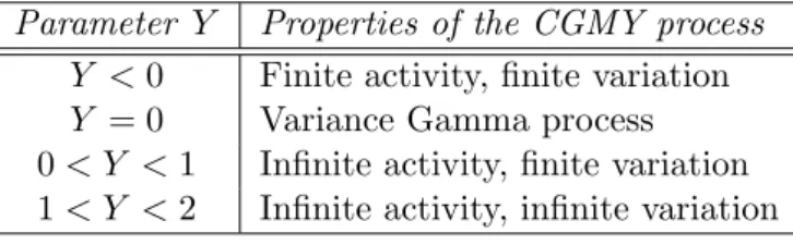
Propositions 2.2 and 2.3 show that the Y parameter also controls the process activity and variation. Table 2.1 sums up this conclusion.

Parameter Y Properties of the CGMY process

Y <0 Finite activity, finite variation

Y = 0 Variance Gamma process 0< Y <1 Infinite activity, finite variation 1< Y <2 Infinite activity, infinite variation

Table 2.1: The parameter Y

We will assume that the dynamics of the latent sovereign value process can be modeled by the CGMY process. In particular, we will set Vt = V0exp (Xt), where Xt is a CGMY process.

In contrast to the VG model, there is no closed form expression for the density of the increments. As a concluding remark, we mention the fact that the CGMY process also admits a time-changed Brownian motion representation, albeit with a time change whose characterization is not as easily attainable as the Gamma process.16

(23)

2.5 Jump-diffusions vs. infinity active, pure jump models 14

2.5 Jump-diffusions vs. infinity active, pure jump models

When choosing a model, the ability to capture empirical phenomena and the underlying economic motivation must be taken into account. Moreover, we must strike a balance between calibration tractability and the number of parameters used: an increase in the latter will improve accuracy at the expense of the former, as several local optima might be found in a non-linear optimization problem.

The jump-diffusion Kou model offers several advantages from this perspective. On the one hand, it introduces jumps with a double exponential distribution, and so it provides both high peaks (capturing the underreaction to new information the market receives) and heavy tails (reflecting overreaction). On the other, it provides analytic tractability through the Laplace transform of the first passage time distribution. However, by using a jump-diffusion process we loose the flexibility a infinite activity process might afford.

We have chosen the CGMY model over a jump-diffusion of the Kou type taking into account the following arguments:

• it captures the stylized empirical behavior of asset returns;

• the pure jump nature of the process is adequate both for stable (an infinite number of “small” jumps in a given time interval) and sudden, low frequency changes in market behavior (at most a finite number of “big” jumps in a given time interval);

• through parameter Y both finite and infinite activity processes are attainable, thus possibly capturing breaches in prevailing market conditions through the crossing of the activity regime;

• even though analytic tractability is lost, in Chapter 3 we will describe an efficient numerical method for the computation of survival probabilities, requiring only the explicit knowledge of the parametric characteristic function (2.9);

• it allies flexibility and numerical tractability to a lower number of parameters.17

Furthermore, we advocate that the pure jump, infinite activity modeling approach is conceptually sounder than the jump-diffusion one. Indeed, the latter adds an orthogonal jump component, essentially capturing “large”, rare jumps that introduce discontinuities, to a diffusion, seizing frequent and small increments. Empirical evidence shows that this can breach the density’s monotonicity, on either side of the increments’ distribution. A pure jump, infinite activity model dispenses with this unconnected building block, effectively merging the small scale behavior (an infinite number of “small” jumps on any compact interval if the L´evy measureν is not bounded around the origin) with the large scale jumps (finitely many, as the L´evy measure is always bounded away from zero). This way, it favors smooth, monotone densities on the right and left of the distribution, displaying skewness and heavy tails.

17_{The CGMY model has four parameters,}_C_,_G_,_M _and_Y_{. Kou’s model has six parameters,}_p_,_θ 1,θ2,λ,

(24)

Chapter 3

Univariate default modeling: the

COS method

In this chapter we address the problem of computing the survival probability under a L´evy first passage structural approach. We will also show how to price Credit Default Swaps (CDSs) and calibrate the underlying model to CDS spreads market data.

Our modeling framework quite naturally casts the survival probability as the price of a barrier option. As such, we can resort to numerical option pricing techniques to compute it. We will apply the Fourier-cosine series option pricing method (Fang and Oosterlee 2008, 2009), henceforth simply referred to as the COS method. This method approximates the transition density fXt|Xs(y|x), truncated to a suitably chosen closed interval [a, b], as a Fourier-cosine series expansion.1 _{The crucial observation behind it is the fact that the}

characteristic function is simply the Fourier transform of the probability density. To obtain the Fourier cosine-series coefficients, we will only need to know an analytic expression for the characteristic function. By using a grid of monitoring points, we can recursively compute the survival probability. This approach is convenient as the L´evy density functionfXt(x) might not be known in closed form, whereas generally we can obtain the characteristic function

φXt(ω).

The material we cover closely follows Fang et al. (2010), where the COS method is used to price CDSs and, through it, calibrate L´evy models. Although we will be applying the COS method to the calibration of the CGMY model, using the parametric expression (2.10), we should emphasize that it could be used at no further cost to any L´evy process whose characteristic function is analytically obtainable.

3.1 Overview

Under a risk-neutral setting, we consider a latent sovereign value process_{Vt, t≥0}, where

Vt=V0eXt

and _{Xt, t≥0} is a L´evy process with X0 = 0. We say that Vt is an exponential L´evy

process.

For a given deterministic recovery rate R _∈(0,1), the time of default is defined as the first-passage time for a barrier set atR V0:

τdef := inf{t≥0 : Vt≤R V0}.

1_{The Fourier-cosine series outperforms the usual Fourier series expansion when approximating functions}

(25)

3.2 Transition density 16

This modeling choice takes the following intuition into account: the larger the recovery rate

R, the lower the cost of defaulting incurred by the sovereign, and so the higher its incentive to formally declare default.2

The survival probability up to time tis then

Psurv(t) =PQ

min

0≤s≤tXs>lnR

=E_Qh1_{_min

0≤s≤tXs>lnR}

i

, (3.1)

where Q denotes the risk-neutral measure. Equation (3.1) can be interpreted as the price of a binary down-and-out barrier (BDOB) option without discounting, with maturityT and barrier level h _≡ lnR. This option pays one unit currency if the trajectory of the process

{Xt}remains abovehup to timeT and zero otherwise. As discussed in Chapter 2, we should note that the distribution of the running-minimum min0≤s≤tXs in (3.1) will not generally be known.

3.2 Transition density

The following proposition is the main result behind the COS method.

Proposition 3.1 (COS formula for the transition density). Let _{Xt, t≥0} be a L´evy

pro-cess with characteristic function ϕlevy(ω, t) := φXt(ω). For 0 ≤ s ≤ t and x, y ∈ [a, b] ⊂ suppf_X_t_|_X_s, the Fourier-cosine series of the transition density f_X_t_|_X_s(y_|x) can be approxi-mated by

fXt|Xs(y|x) = 2

b₋a

N−1

X

k=0

′

Re

ϕlevy

_kπ

b₋a, t−s

eikπxb−−aa

·cos

kπy−a

b₋a

+εf, (3.2)

where P′ means that the first term is halved. The error term εf comes both from truncating

the support of f_X_t_|_X_s to the interval [a, b] and taking only the first N terms of the series expansion.

Appendix A.1 presents the proof of this result.

3.3 Survival probability

In this section we will show how the transition density approximation formula (3.2) can be used to compute the survival probability Psurv(t) as the price of a discretely monitored binary down-an-out barrier option.

We start by defining a set of M pre-specified observation dates,

T ={t₀, t₁, . . . , tM}, t0< t1 <· · ·< tM, tm =m·∆t, m= 0,1, . . . , M,

where the value of the L´evy process _{Xt, t≥0} will be monitored and compared with the barrier level set at h_≡lnR. We will denote the final observation date byτ =tM.

The survival probability for the whole period

Psurv(τ) =EQ

" _M Y

m=0

1_{Xtm>h}

#

(3.3)

2_{The default barrier is defined in terms of a relative decrease of the latent sovereign value process so as to}

avoid the need to explicitly estimateV0. Following the remarks made in Section 2.1.4, we acknowledge the

(26)

3.3 Survival probability 17

can be obtained recursively. Define

p(x, tM) :=1{x>h}

p(x, tm) :=EQ

h

1_{_X

tm+1>h}

Xtm =x

i

=

Z +∞

h

fX_tm₊₁|Xtm(y|x)p(y, tm+1)dy, (3.4)

for m = M ₋1, . . . ,0. Then, by taking conditional expectations on the values of Xtm in

(3.3), we get

Psurv(τ) =p(0, t0), (3.5)

because, from our definition of the sovereign value processVt,X0= 0.

We will now use the COS expansion of the transition density from the previous section to approximate the recursive integral in (3.4).

Proposition 3.2 (COS formula for the survival probability). Plugging (3.2) into (3.4), we get the following recursive relationship:

p(x, tm) = N−1

X

k=0

′

φk(x)Pk(tm+1),

where

φk(x) := Re

ϕlevy

_kπ

b₋a,∆t

eikπxb−−aa

Pk(tm+1) :=

2

b₋a

Z b h

cos

kπy−a

b₋a

p(y, tm+1)dy. The survival probability can then be approximated by

Psurv(τ) = N−1

X

k=0

′

φk(0)Pk(t1). (3.6)

The proof can be found in Appendix A.2.

We should note that _{Pk(t1)}kN=0−1 are simply the Fourier-cosine coefficients of p(y, t1).

In the next section we will show how these can be computed recursively.

3.3.1 Backwards recursion

The Fourier coefficients {Pk(tm)}Nk=0−1 can be obtained from {Pk(tm+1)}Nk=0−1 the following

way:

Pk(tm) = 2

b₋a

Z b h

cos

kπy−a

b₋a

p(y, tm)dy

= 2

b₋a

Z b h

cos

kπy−a

b₋a

N−1

X

l=0

′

φl(x)Pl(tm+1)dy

= N−1

X l=0 ′ Re ϕlevy lπ b₋a,∆t

ωkl

Pl(tm+1),

where we have defined

wkl:= 2

b₋a

Z b h

eilπyb−−aa_cos

kπy−a

b₋a

(27)

In matrix notation, the previous recursive relationship becomes

P(tm) = Re{ΩΛ}P(tm+1), (3.7)

where

Ω = (ωkl)Nk,l−=01 and Λ = diag

ϕlevy

lπ b₋a,∆t

N−1

l=0

is a diagonal matrix.

So, the computation of the survival probability up toτ =tM using the COS formula (3.6) boils down to obtaining the vector of Fourier-cosine coefficients P(t1) from the backwards

recursion

P(t1) = Re{ΩΛ}M−1P(tM). (3.8) The recursion base vector of Fourier-cosine coefficients for p(x, tM) = 1{x>h}, P(tM), can be calculated explicitly as

Pk(tM) = 2

b₋a

Z b h

cos

kπy−a

b₋a

p(y, tM)

| {z }

1{y>h}

dy = ( 2 kπ h

sin (kπ)₋sinkπh_b₋−_aai k₆= 0

2

b−a(b−h) k= 0,

(3.9)

but getting the coefficients P(t1) using (3.8) is computationally expensive.

In the next section we will describe an alternative, more efficient way to compute (3.8) using the Fast Fourier Transform (FFT) algorithm.

3.3.2 Computation using the FFT

The crucial observation is the fact that the matrix Ω can be expressed as the sum of two matrices with special properties. To see this, first define

wj :=

(

iπb_b−₋h_a j= 0

exp(ijπ)−exp(ijh_b₋−_aaπ)

j j6= 0.

Proposition 3.3 (Representation of Ω as the sum of Hankel and Toeplitz matrices). The

matrix Ωcan be written as

Ω =−i

π(H+T), where H =       

w₀ w₁ _{· · ·} wN−2 wN−1 w1 w2 · · · wN

..

. . .. . .. . .. ...

wN−2 wN−1 · · · w2N−3 wN−1 · · · w2N−3 w2N−2

      

and T =

      

w₀ w₁ _{· · ·} wN−2 wN−1 w−1 w0 · · · wN−2

..

. . .. . .. . .. ...

w2−N w3−N · · · w1 w1−N · · · w−1 w0

      

are, respectively, a Hankelmatrix3 _{and a} _Toeplitz _matrix,4 _both _N_×_N.

3_{A Hankel matrix}_H_{= (}_h

ij)N_i,j₌₁is a square matrix with constant positive slope diagonals, i.e., such that

hij=hi−1,j+1.

4_{A Toeplitz matrix}_T _{= (}_t

(28)

Details on the proof can be found in Fang and Oosterlee (2009), pp. 8-9.

The basic recursion for the recovery of the Fourier-cosine coefficients (3.7) can then be rewritten5 as

P(tm) = 1

πIm{(H+T)u(tm+1)}, (3.10)

withu(tm+1) := (uj(tm+1))N_j₌₀−1 such that u₀(tm+1) :=

1

2ϕlevy(0,∆t)P0(tm+1) (3.11)

uj(tm+1) :=ϕlevy

jπ b₋a,∆t

Pj(tm+1), j= 1, . . . , N −1. (3.12)

Due to the structure of Hankel and Toeplitz matrices, their product by a vector can be expressed as a circular convolution. This will allow us to recover P(tm) using the FFT algorithm, thus significantly reducing the complexity of the computation.

Definition 3.1 (Circular convolution). Take two vectors of the same dimension, x and y,

and denote by _D the discrete Fourier transform (DFT) operator. The circular convolution

of x and y is

x⊛y:=D−1{D(x)· D(y)}.

Proposition 3.4. Let H andT be, respectively, Hankel and Toeplitz N _×N matrices.

1. The matrix-vector product H_·u can be obtained as

H_·u= [wH ⊛uH]

←−

N

with the following vectors of dimension 2N

wH := [w2N−1, w2N−2, . . . , w1, w0]T (3.13)

uH := [0, . . . ,0, u0, u1, . . . , uN−1]T, (3.14) where [x]←N− denotes taking the vector of the first N elements of x, in reversed order.

2. The matrix-vector product T _·u can be obtained as

T_·u= [wT ⊛uT]

− →

N

with the following vectors of dimension 2N

wT := [w0, w−1, . . . , w1−N,0, wN−1, wN−2, . . . , w1]T (3.15)

uT := [u0, u1, . . . , uN−1,0, . . . ,0,]T, (3.16)

where [x]−→N denotes taking the vector of the first N elements of x.

The proof can be found in Fang and Oosterlee (2009) – first part – and Almendral and Oosterlee (2007) – second part.

Remark (Decreasing the complexity of the computation of the Fourier-cosine coefficients).

The matrix-vector products in equation (3.7) involve O N2 operations. Using (3.10) and the previous proposition, we can reduce it to _O(Nlog₂N), as the complexity of the FFT algorithm is of this order.

(29)

3.3.3 The COS algorithm

This sections outlines the main steps of the COS algorithm to compute the survival proba-bility Psurv(τ), τ =tM.

Recursion base

Step 1 Compute P(tM), the vector of Fourier-cosine coefficients of p(x, tM), from (3.9); Step 2 Build the vectorswH and wT from (3.13) and (3.15);

Step 3 Compute the FFTsdH =D(wH) and dT =D(wT);

Recursion loop

Form=M, . . . ,2, perform the following steps:

Step 4 Compute the vectoru(tm) from (3.11) and (3.12); Step 5 Compute uH(tm) from (3.14);

Step 6 Compute the matrix-vector products

H_·u(tm) =

D−1{dH · D[uH(tm)]}

←N−

, T _·u(tm) =

D−1{dT · D[uH(tm)]}

−→N ;

Step 7 ObtainP(tm−1) from (3.10);

At the end of the loop, we will have recovered P(t1), the vector of Fourier-cosine

coeffi-cients of p(x, t1).

Survival probability

Step 8 Compute the survival probability Psurv(τ) from (3.6). Improving the computational efficiency

Coefficients wj The coefficientswj must be computed for

j=₋(N ₋1), . . . ,₋1

| {z }

N−1 terms

, j= 0, j= 1, . . . , N ₋1

| {z }

N−1 terms

, j=N, . . . ,2(N₋1)

| {z }

N−1 terms .

To do so in an efficient way, we note that, from the definition, w−j =−wj, and so we can getwj forj=−(N−1), . . . ,1 from wj,j= 1, . . . , N −1. Additionally,

wj+N =

exp (iN π) exp (ijπ)₋expiNh_b₋−_aaπexpijh_b₋−_aaπ

N +j ,

so the factors exp (ijπ) and expijh_b₋−_aaπneed to be computed only once.

FFT As uH is simply uT shifted N positions to the right, the FFT dH can be computed from dT, using the shift property of the discrete Fourier transform:

D(uH) =sgn· D(uT), sgn=

(30)

3.4 Pricing Credit Default Swaps 21

3.4 Pricing Credit Default Swaps

In a Credit Default Swap (CDS) contract, the protection buyer transfers the credit risk of a reference entity’s underlying asset to the protection seller by paying a premium until a default event occurs or the maturity of the contract is reached. The protection seller makes no payments in the latter case, while it covers the losses in case of default. TheCDS spread

is the yearly rate paid by the protection buyer. It thereby provides the market aquantitative measure of the implicit credit riskiness of the reference entity.

Let us denote byT the maturity of a CDS contract with yearly spreadc. We will assume a constant risk-free interest rater in [0, T], and that a deterministic recovery rateR_∈(0,1) is known in advance.6

Proposition 3.5. The fair CDS spread can be approximated as

c∗ = (1₋R)

"

1₋e−rTPsurv(T)

PJ

j=0wje−rt˜jPsurv ˜tj·∆t

−r

#

, (3.17)

where ˜tj =j·∆t, j= 0, . . . , J, ∆t= T_J, is a suitable discretization of the interval[0, T], and

wj = 1₂ for j= 0, J, wj = 1 otherwise. We prove this result in Appendix A.3.

Equation (3.17) shows that we can numerically approximate the fair CDS spread by computing the survival probability Psurv(˜tj) for every ˜tj. We will use the COS survival probability formula (3.6) for a given L´evy process, as specified by its parametric characteristic function. In the next section, we will define the procedure to calibrate the parameters of the latter to market CDS spread data.

Remark (Simultaneous computation of survival probabilities). The choice of the points ˜tj

used to approximate the integral on the CDS pricing formula can be made in such a way that the computation ofall the survival probabilitiesPsurv ˜tj

is achievable simultaneously. For this, we simply need to ensure that the J points˜tj J_j₌₁ lie in the set ofM observation dates {tj}M_j₌₀ used in the discretization of the barrier option. If ˜ti <t˜j are two such points, we have ti = _Mktj for some k ∈ N, and so the Fourier-cosine coefficients of the survival probability Psurv(ti) were already obtained during the computation of Psurv(tj):

P˜ti(t1) =Pt˜j(tM−k+1).

3.5 Calibration

Letϕlevy(ω, t;θ1, . . . , θn) be the characteristic function of the underlying L´evy process{Xt}t≥0,

with parametersθ₁, . . . , θn.

On a given day, we observe the market CDS spreads cmarket(Ti) for a set ofmmaturities

T1<· · ·< Tm. We will calibrate the L´evy model to the market data by minimizing the root mean square error function

RMSE(θ1, . . . , θn) =

v u u t

m

X

i=1

(cmarket(Ti)−clevy(Ti))2

m , (3.18)

whereclevy(Ti) is computed using the COS formula (3.17). The optimal choice of parameters, argmin_θ₁_,...,θ_nRMSE(θ1, . . . , θn),

(31)

3.6 Parameters 22

3.6 Parameters

Discretization parameters

Following the error analysis discussed in Fang et al. (2010), we use the authors’ proposed choice of discretization parameters:

Parameter Description Value

N Terms in Fourier-cosine series expansion N = 210 M Monitoring dates for discrete BDOB option M = 48T

J Discretization points for CDS pricing J = M

4

Table 3.1: Discretization parameters

N The number of terms in the Fourier-cosines series expansion N is chosen as a power of two to allow the use of the FFT algorithm; we use N = 210= 1024 terms;

M We will be using weekly-monitored survival probabilities; M = 48T (or, equivalently, ∆t= ₄₈1 ) means we are considering 48 “trading weeks” in a year;

J The authors find the CDS pricing formula not to be very sensitive to this parameter; the choice J = M

4 (as opposed toJ =M) is used to improve computational efficiency.

Truncation range

The truncation range of the support of the transition density f_X_t_|_X_s should made be large enough for the approximation error term in (3.2) to stem mainly from taking onlyN terms in the Fourier-cosine series (Fang et al. 2010). The authors find the following definition to be wide enough:

[a, b] :=

c1±L

q

c2+√c2

,

wherecj is thej-th cumulant ofXt(cf. Fang and Oosterlee 2009, appendix B) and parameter

L_∈[7.5,10]. We have usedL= 10.

Recovery rate

We have decided from the beginning that taking a stochastic modeling approach to the re-covery rate parameterR would be out of our work’s scope. Arguably, we could assume that

R follows a given parametric distribution, with minimal implementation effort.7 _However,

such a modeling choice would be made mainly on practical arguments rather than sound eco-nomic reasoning. Moreover, we would have to calibrate the distribution parameters making some crude assumptions: data on sovereign loss given default is not only scarce, precluding any statistically significant analysis, but also heterogeneous, as final recovery rates will be determined by the specific economic and political circumstances leading to default.

Because we are strictly focused on Euro area sovereigns, we will use available data on the 2012 Greek and 2013 Cypriot defaults as a proxy for a non-deterministic Euro area recovery rate. These default events have taken the form of distressed debt exchanges8, as opposed to missing payments of coupons or principal. In its report on Sovereign Default and Recovery

Rates, 1983–2013 (Moody’s Investors Service 2014), Moody’s measures the recovery rate as

7_{Two possible models are the Beta distribution (with support [0}_,_{1]) or an appropriate map of a distribution}

with supportRto [0,1] (Sch¨onbucher 2003, Section 6.1.6).

(32)

3.6 Parameters 23

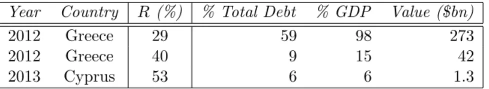
the ratio of the present value9 of the new, restructured securities to the original ones. Table 3.2 presents the estimated recovery rates and the value of the restructured securities. The latter is also expressed as a percentage of both the country’s total debt and its GDP.

Year Country R (%) % Total Debt % GDP Value ($_bn)

2012 Greece 29 59 98 273

2012 Greece 40 9 15 42

2013 Cyprus 53 6 6 1.3

Table 3.2: 2012–2013 Euro area default events. Source: Moody’s Sovereign Default and Recovery Rates, 1983–2013.

Taking into account the sheer dimension of the first 2012 Greek restructuring10, we will choose a deterministic recovery rate of 30%. The data on the Cyprus default suggests that our choice is possibly conservative.

9_{Using the original securities’ yield to maturity at the time of the exchange.}

10_{The largest in history, measured as the nominal amount of debt exchanged, the percentage of total debt}

(33)

Chapter 4

The dataset

As we have seen in the previous chapter, to calibrate a L´evy model from market CDS spreads we will need to minimize the root mean square error (3.18) of the theoretical spreads vis-a-vis the observed ones. This means that, besides fetching market CDS data, we will need information on the risk-free yield curve to use the pricing formula (3.17).

We have collected from Bloomberg the series of daily bid and ask USD-quoted CDS spreads with maturities T _{∈ {}1,3,5,7,10_} years (Y), spanning the period from 01-01-2010 to 28-02-2014, for the Euro-area Portuguese (PT), Irish (IE), Italian (IT), Greek (GR) and Spanish (SP) sovereigns. This time frame covers the onset of the Euro-area sovereign debt crisis, its peak, and the early stages of the ongoing recovery. To remove possible weekday effects, our calibration will be based only on weekly Wednesday mid-quotes.

We used USD-quoted CDS spreads because the corresponding Euro-quoted ones did not cover extensively neither the period in question nor a representative set of tenors.1

We recognize that, ideally, Euro-quoted CDS contracts should be used, as the underlying sovereign debt is Euro-denominated. However, the USD dataset was judged preferable, as it would lead to a statistically more significant calibration. We are thus taking the perspective of an American investor in Euro-area sovereign debt. Furthermore, as the recovery rate R

is purely exogenous, we will assume that it covers not only the notional loss given default

but also any foreign exchange losses. This simplifying assumption will give leeway to the

use of USD-quoted spreads as a pure credit risk measure, free of any implicit currency risk component.

01/100 01/11 01/12 01/13 01/14

500 1000 1500 2000 2500

Date

Spread (bps)

PT CDS Spreads

1Y 3Y 5Y 7Y 10Y

01/100 01/11 01/12 01/13 01/14

500 1000 1500 2000 2500

Date

Spread (bps)

IE CDS Spreads

1Y 3Y 5Y 7Y 10Y

Figure 4.1: Daily mid-quotes for Portuguese (PT) and Irish (IE) CDS spreads

Figure 4.1 shows that the Portuguese and Irish CDS spreads had a somewhat similar

1_{Only the 5 and 10 years tenors were generally available. This is an indication of the Euro denominated}

M ESTRADO A CTUARIALS CIENCE T RABALHOF

M

ESTRADO

A

CTUARIAL

S

CIENCE

T

RABALHO

F

INAL DE

M

ESTRADO

DISSERTAÇÃO

MODELING SOVEREIGN DEBT WITH LÉVY PROCESSES

GONÇALO ANDRÉ NUNES PEREIRA

M

ESTRADO EM

A

CTUARIAL

S

CIENCE

T

RABALHO

F

INAL DE

M

ESTRADO

DISSERTAÇÃO

MODELING SOVEREIGN DEBT WITH LÉVY PROCESSES

GONÇALO ANDRÉ NUNES PEREIRA

O

RIENTAÇÃO

:

R

AQUEL

G

ASPAR

J

OÃO

G

UERRA

Acknowledgments

Contents

List of Figures

List of Tables

Chapter 1

Introduction

Chapter 2

Structural credit risk modeling

under L´

evy dynamics

2.1

The structural approach

2.2

Financial modeling with L´

evy processes

2.3

Jump-diffusion processes

2.4

Infinite activity, pure jumps processes

2.5

Jump-diffusions vs. infinity active, pure jump models

Chapter 3

Univariate default modeling: the

COS method

3.1

Overview

3.2

Transition density

3.3

Survival probability

3.4

Pricing Credit Default Swaps

3.5

Calibration

3.6

Parameters

Chapter 4

The dataset