DEPARTAMENTO DE FÍSICA
Sensitivity correction of images obtained
with the prototype Clear-PEM in pre-clinical
environment
Ana Cristina da Fonseca Teixeira
Dissertation presented at
Faculdade de Ciências e Tecnologia
Universidade Nova de Lisboa
to obtain a Master Degree in Biomedical
Engineering
Advisors: Professor Dr. Pedro Almeida
Professor Dr. Nuno Matela
Acknowledgments
This work was carried out at Instituto de Biofísica e Engenharia Biomédica da Faculdade de Ciências da Universidade de Lisboa (IBEB). I would like to express my sincere gratitude to those who have supported me and contributed to this thesis.
First and foremost, I would like to thank my advisor, Professor Pedro Almeida, for the opportunity he gave me to choose my own work and join his Molecular Imaging research group, despite being a student at a different university.
I would also like to make a special reference to my other advisor, Professor Nuno Matela. Thank you, not only for your constant assistance and guidance in this study but also for all the support, patience and friendship! It has been great working with you.
To Nuno Oliveira, I would like to show my gratitude for all the work developed in the creation and maintenance of Quasimanager, for it sure made my work a lot easier.
For the most cheering and enthusiastic person at IBEB, Professor Ducla-Soares, I want to thank for all the encouragement and kind words. You make us all want to “grow up” to be like you.
To all my colleagues and friends at IBEB, for all the laughter and the good times at
our “i-events”, but also for the help, the advice and the encouraging, a huge thank you. Especially to Pedro, my editor, for all your kind words of friendship and support; to Miguel, even with all the kicking under the table, it was great working with you on this adventure
outside “their” FCT; to Liliana, your strength and will to keep everything moving forward is unbelievable, thank you for your inspiration. But also to Ricardo, Henrique, Beatriz, and everybody else at IBEB.
Considering that this work was the end of a cycle, I would really like to mention my truest friends, who kept me going in this last five years, even during some hard times... A big thank you to Kiko, Joana, Miguel Abreu, Ana Patrícia, João and Miguel Gonçalves, for your friendship and for everything we have been through, together!
years, cheering me up and giving me strength to carry on. Thank you for all the good times (and after 18 years, there are a lot) for all your friendship and all your love.
Also to our Gang: girls, thank you for being there, even after all these years.
I would also like to thank the most important people in my life: my parents. For everything you have ever done for me, for all your love, all the support and encouragement and for teaching me to always have a thirst for knowledge: Thank you!
To my grandparents, Maria e António, I want to thank for always believing in me and putting me first, and for your unconditional love.
Last, but definitely not least, to Kiko. For all the unnecessary worrying, the friendship, the company, the talks, the love... You are truly my best friend, and for that I thank you!
Abstract
Nuclear medicine has, when compared to anatomical imaging techniques, the great advantage of identifying the metabolic activity of the cells, hence becoming a great option for tumour identification.
A new technology in this area is Positron Emission Mammography (PEM) that follows the same physical basics of Positron Emission Tomography (PET). The Clear-PEM project, a Portuguese research project, uses this technology and, in alternative to the whole-body exam, only the breast is examined, using two detector plates that rotate around the breast to detect radiation. The prototype has the ability to perform a complementary exam of the axillary region. This scanner is designed to detect small lesions or tumours in early stages, with high resolution and high sensitivity.
After the acquisition, the data undergoes a process of reconstruction and corrections. It is our job to study which parameters should be adjusted in order to get the best contrast between lesions and the breast background, as well as meeting the high resolution standards we set to achieve.
This work consisted in the correction of some characteristics that might influence image quality. The first correction made was the elimination of the presence of the gaps between the detector crystals’ effects, resulting in the enhancement of the image Signal-to-Noise Ratio (SNR).
By varying the energy window of the image acquisitions, it was possible to minimize the effect of scattered photons, and varying the timing window minimized the effect of random coincidences.
Resumo
A medicina nuclear tem, sobre as técnicas de imagem anatómica, a grande vantagem de mostrar a actividade metabólica das células, característica esta que é uma mais-valia para a identificação de tumores.
Uma nova tecnologia nesta área é a Mamografia por Emissão de Positrões, que segue os princípios físicos de um exame de Tomografia por Emissão de Positrões. O projecto Clear-PEM, fruto de investigação portuguesa, adopta esta tecnologia e, em alternativa ao exame de corpo inteiro, efectua um exame apenas à mama, recorrendo a dois detectores planares, que rodam em torno da mesma. O protótipo tem também a possibilidade de fazer exames à axila. Pretende-se que, em ambiente clínico, venha a apresentar uma alta resolução, alta sensibilidade e que seja capaz de detectar pequenas lesões e tumores em baixos estágios de desenvolvimento.
Após a aquisição, os dados terão de ser reconstruídos e corrigidos para que se obtenha uma imagem. Este trabalho consiste em estudar quais as características a ajustar de forma a conseguir o melhor contraste entre possíveis lesões e o fundo da mama, bem como garantir que vamos de encontro aos padrões de alta resolução propostos.
O trabalho consistiu na correcção de vários parâmetros que influenciam a qualidade da imagem obtida. A primeira correcção efectuada foi a eliminação de artefactos resultantes da presença de gaps entre os cristais, resultando numa melhoria da Razão Sinal-Ruído da imagem.
Fazendo variar a janela de energia da aquisição das imagens, foi possível minimizar o efeito dos fotões Compton, e fazendo variar a janela de tempo minimizou-se o efeito de coincidências aleatórias.
Acronyms and abbreviations
APD Avalanche Photodiode
ART Algebraic Reconstruction Technique CT Computed Tomography
DOI Depth of Interaction FOV Field of View
FBP Filtered Backprojection FWHM Full Width at Half Maximum
LOR Line of Response
ML-EM Maximum Likelihood - Expectation Maximization MRI Magnetic Resonance Imaging
OS-EM Ordered Subsets - Expectation Maximization PEM Positron Emission Mammography
PET Positron Emission Tomography ROI Region of Interest
SNR Signal to Noise Ratio
xv
Contents
Acknowledgments vii
Abstract ix
Resumo xi
Acronyms and abbreviations xiii
Contents xv
List of Figures xvii
List of Tables xxi
Chapter 1. Introduction 1
Chapter 2. Positron Emission Tomography 5
2.1. Nuclear Medicine ... 5
2.2. Physical basis ... 5
2.2.1.Positron Emission ... 6
2.2.2.Annihilation ... 7
2.3. Interactions with matter ... 9
2.3.1.Photoelectric Effect ... 9
2.3.2.Compton Scattering ... 10
2.3.3.Photon Attenuation ... 11
2.4. Positron Emission Mammography ... 12
Chapter 3. The Clear-PEM Scanner 15 3.1. The scanner ... 15
3.2. Radiation Detectors... 16
3.2.1.Scintillators and Avalanche Photodiodes ... 16
3.2.2.Coincidence Detection ... 17
Chapter 4. Data Acquisition and Image Reconstruction 19 4.1. Organization of Acquired Data ... 19
4.1.1.Data Rebinning ... 20
4.1.2.Linograms ... 21
4.2. Image Reconstruction ... 23
4.3. Analytic Image Reconstruction ... 24
4.4. Iterative Image Reconstruction ... 24
4.4.1.3.The Tube-Driven Method ... 27
4.4.2. The Algebraic Reconstruction Technique (ART) ... 29
4.4.3. The Maximum Likelihood - Expectation Maximization (ML-EM) ... 30
4.4.4. The Ordered Subsets - Expectation Maximization (OS-EM) ... 30
Chapter 5. Sensitivity Correction 33 5.1. Sensitivity and Detector Gaps ... 33
5.2. Correction Based on the Planar Source Acquisition ... 35
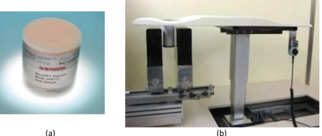
5.2.1. The Phantoms used ... 35
5.2.1.1.Planar Source ... 35
5.2.1.2.Cylindrical phantom ... 36
5.2.2. Threshold Definition ... 36
5.2.3. Studies in the Cylindrical Phantom ... 38
5.2.3.1.Reconstruction Assessment ... 38
5.2.3.2.Linogram Assessment ... 42
5.2.4. Validation with Clinical Data ... 47
5.2.4.1.Image Noise ... 48
5.2.4.2.Presence of High Intensity Pixels ... 50
5.2.5. Discussion ... 53
5.3. System Matrix Correction ... 53
5.3.1. Analytical Linogram ... 54
5.3.2. Validation with Planar Source ... 56
5.3.3. Incorporation on the System Matrix Calculation ... 57
Chapter 6. Random Correction 61 6.1. Timing Window ... 61
6.2. Random Correction ... 62
6.2.1. Image Contrast ... 64
6.2.2. Image Noise ... 70
6.2.3. Presence of High Intensity Pixels ... 72
6.2.4. Discussion ... 73
Chapter 7. Scattered Correction 75 7.1. Energy Window ... 75
7.2. Scattered Correction ... 76
7.2.1. Image Contrast ... 76
7.2.2. Image Noise ... 77
7.2.3. Spatial Resolution Studies ... 79
7.2.2.1.Point Source Phantom ... 79
7.2.2.2.FWHM ... 80
7.2.4. Discussion ... 83
Chapter 8. Main Discussion and Conclusions 85
Bibliography 87
List of Figures
Figure 2.1: Positron decay [17]. ... 6
Figure 2.2: Annihilation reaction [17]. ... 8
Figure 2.3: Photoelectric effect [17]. ... 9
Figure 2.4: Predominant type of interaction for various combinations of incident photons and absorber atomic numbers [17]. ... 10
Figure 2.5: Compton scattering [17]. ... 10
Figure 3.1: Clear-PEM breast acquisition [21]. ... 15
Figure 3.2: Clear-PEM axillary region acquisition [21]. ... 15
Figure 3.3: Schematic drawing of the Clear-PEM scanner [18]. ... 17
Figure 3.4: Types of coincidences detected in a PET imaging system: (a) Scattered coincidences; (b) Random coincidences; (c) True coincidences. Figure adapted from [23]. ... 17
Figure 4.1: Single Slice Rebinning. ... 21
Figure 4.2: Definition of linogram coordinates. Figure adapted from [28]. ... 22
Figure 4.3: Linogram example. Figure adapted from [28]... 22
Figure 4.4: (a) Detectable LORs with v=0; (b) Detectable LORs with v=vmin and v=vmax; (c) Detectable LORs with u=umin and u=umax; (d) Detectable region of a linogram. Figure adapted from [28]. ... 23
Figure 4.5: Backprojection. The image reconstruction quality increases with the number of projections [23]. ... 24
Figure 4.6: Iterative reconstruction process. Figure adapted from [23]. ... 25
Figure 4.7: Possible intersections between a TOR and a pixel: (a) a trapezium, (b) the entire pixel except one or two triangles, or (c) one triangle. ... 28
Figure 4.8: Variables used to calculate the area of intersection between the TOR and the pixel. ... 29
event. ... 34 Figure 5.3: Picture of the planar source during its acquisition in the Clear-PEM
prototype. ... 35 Figure 5.4: (a) 68Ge cylindrical phantom. (b) Picture of the phantom inside the support
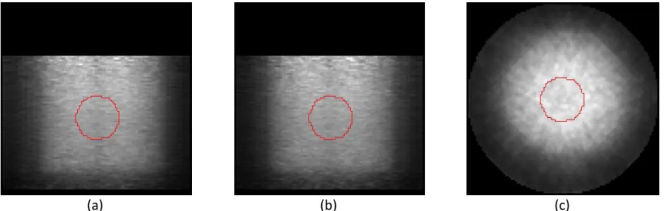
used for the acquisition. ... 36 Figure 5.5: Image reconstruction of the cylindrical phantom without sensitivity
corrections in the (a) yz and (b) xy planes. ... 36 Figure 5.6: Representation of the ROIs used in the study for (a) yz , (b) xz and (c) xy
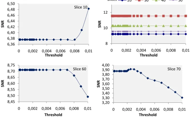
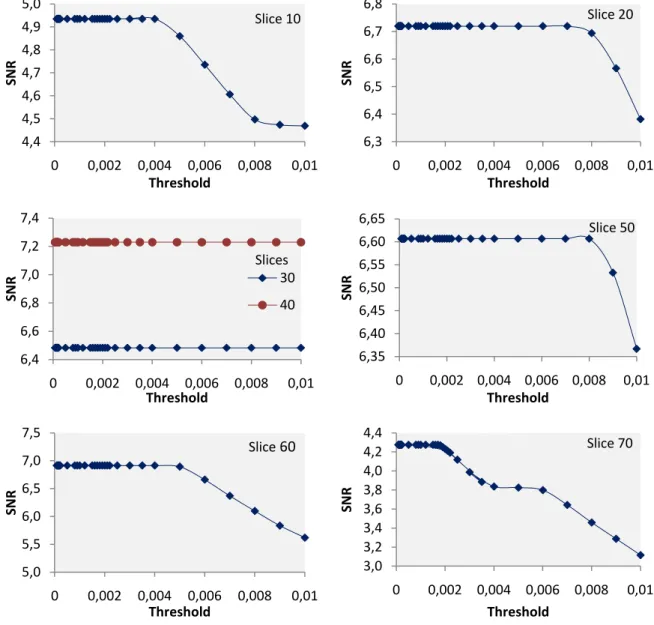
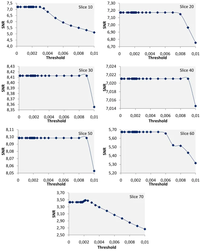
views. ... 39 Figure 5.7: SNR values obtained for the 50th slice of the xz, yz and xy plane of the
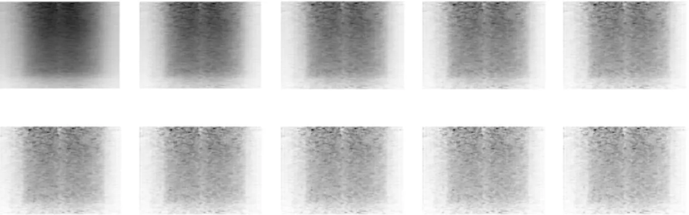
cylindrical phantom, with a 0.001 threshold, during 10 iterations. ... 40 Figure 5.8: Images reconstructed with OS-EM 2D from the 1st to the 10th iteration, with
the same sensitivity correction threshold. ... 40 Figure 5.9: SNR values obtained for the 50th slice of the xy plane of the cylindrical
phantom after 3 iterations. ... 41 Figure 5.10: SNR values obtained for the 50th slice of the xz plane of the cylindrical
phantom after 3 iterations. ... 41 Figure 5.11: SNR values obtained for the 50th slice of the yz plane of the cylindrical
phantom after 3 iterations. ... 41 Figure 5.12: SNR values obtained for the 72nd slice of the xy plane of the cylindrical
phantom after 3 iterations. ... 42 Figure 5.13: Linograms of the cylindrical phantom acquisition without sensitivity
corrections for (a) yz , (b) xz and (c) xy planes. ... 42 Figure 5.14: Representation of the ROI drawn in the linograms. ... 43 Figure 5.15: SNR values obtained for a ROI of the 𝒙𝒚 plane of the cylindrical phantom
linogram. ... 43 Figure 5.16: Representation of a profile analysis in an uncorrected linogram. ... 44 Figure 5.17: Representation of a profile analysis in a corrected linogram with a 0.002
threshold. ... 44 Figure 5.18: SNR values obtained for a profile of the xy plane of the cylindrical phantom
linogram. ... 45 Figure 5.19: SNR values obtained for a profile of the xy plane of the cylindrical phantom
linogram. ... 46 Figure 5.20: Image reconstruction of the first clinical case in the (a) yz, (b) xz and (c) xy
correction (reverse grey scale)... 48
Figure 5.22: Central ROI marked on clinical cases 1 a 3. ... 48
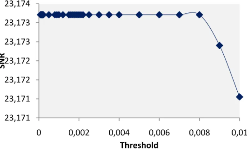
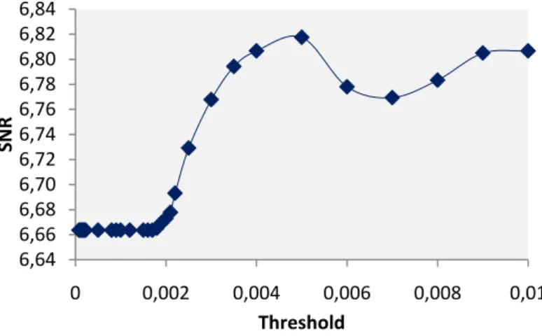
Figure 5.23: SNR values obtained with a central ROI for slice 44 of clinical case 1. ... 49
Figure 5.24: SNR values obtained with a central ROI for slice 53 of clinical case 1. ... 49
Figure 5.25: SNR values obtained with a central ROI for slice 41 of clinical case 3. ... 49
Figure 5.26: SNR values obtained with a central ROI for slice 52 of clinical case 3. ... 50
Figure 5.27: Image reconstruction of the same slice corrected with different thresholds. .... 51
Figure 5.28: Rectangular ROI marked on clinical cases 1 a 3. ... 51
Figure 5.29: Maximum values obtained with a bottom rectangular ROI for clinical case 1. ... 52
Figure 5.30: Maximum values obtained with a bottom rectangular ROI for clinical case 3. ... 52
Figure 5.31: Variables definition for lengths of the LORs in a linogram. ... 54
Figure 5.32: Representation of the analytic linogram created. ... 56
Figure 5.33: Result of difference (c) between the analytic linogram (a) and the planar source acquisition (b). ... 57
Figure 5.34: Cylinder reconstruction with (a) analytic linogram and (b) the planar source acquisition with a 0.005 threshold. ... 58
Figure 5.35: Image reconstruction of clinical 1 with (a) analytic linogram and (b) the planar source acquisition with a 0.005 threshold... 58
Figure 5.36: Image reconstruction of clinical 3 with (a) analytic linogram and (b) the planar source acquisition with a 0.005 threshold... 59
Figure 6.1: Result of difference (c) between the regular reconstruction (a) and the reconstruction of the random corrected data (b) with an 8 ns timing window. ... 63
Figure 6.2: Circular ROIs marked on clinical cases 1, 3, 4 and 5. ... 65
Figure 6.3: Rectangular ROIs marked on clinical cases 1, 3, 4 and 5. ... 65
Figure 6.4: Contrast values obtained for Clinical 1 with a circular ROI. ... 66
Figure 6.5: Detail of the contrast values obtained for Clinical 1 with a circular ROI. ... 66
Figure 6.6: Contrast values obtained for Clinical 3 with a circular ROI. ... 66
Figure 6.7: Detail of the contrast values obtained for Clinical 3 with a circular ROI. ... 67
Figure 6.8: Contrast values obtained for Clinical 5 with a circular ROI. ... 67
Figure 6.9: Detail of the contrast values obtained for Clinical 5 with a circular ROI. ... 67
Figure 6.10: Contrast values obtained for Clinical 1 with a rectangular ROI. ... 68
Figure 6.11: Contrast values obtained for Clinical 3 with a rectangular ROI. ... 69
Figure 6.12: Detail of the contrast values obtained for Clinical 3 with a rectangular ROI. ... 69
Figure 6.13: Contrast values obtained for Clinical 5 with a rectangular ROI. ... 69
Figure 6.14: Detail of the contrast values obtained for Clinical 5 with a rectangular ROI. ... 70
Figure 6.17: SNR values obtained with a circular ROI for clinical case 5. ... 71
Figure 6.18: Maximum values obtained with a bottom rectangular ROI for clinical case 1. ... 72
Figure 6.19: Maximum values obtained with a bottom rectangular ROI for clinical case 3. ... 72
Figure 6.20: Maximum values obtained with a bottom rectangular ROI for clinical case 5. ... 73
Figure 7.1: Contrast values obtained for Clinical 1 with a circular ROI. ... 76
Figure 7.2: Contrast values obtained for Clinical 3 with a circular ROI. ... 77
Figure 7.3: Contrast values obtained for Clinical 5 with a circular ROI. ... 77
Figure 7.4: SNR values obtained with a circular ROI for clinical case 1. ... 78
Figure 7.5: SNR values obtained with a circular ROI for clinical case 3. ... 78
Figure 7.6: SNR values obtained with a circular ROI for clinical case 5. ... 78
Figure 7.7: Image detail of the reconstruction of the point source phantom without corrections in the (a) yz, (b) xz and (c) xy planes. ... 80
Figure 7.8: Profile (a) and Gaussian curve fit (b) for the yz plane of the point source... 81
Figure 7.9: Profile (a) and Gaussian curve fit (b) for the xz plane of the point source. ... 81
Figure 7.10: Profile (a) and Gaussian curve fit (b) for the xy plane of the point source. ... 81
Figure 7.11: FWHM values for the point source phantom in plane yz. ... 82
Figure 7.12: FWHM values for the point source phantom in plane xz. ... 82
List of Tables
Table 2.1: Mass and Charge Properties of Nucleons, Electrons and Positrons [15]. ... 6
Table 2.2: Some commonly used radioisotopes. ... 12
Table 5.1: Comparison between the SNR values obtained with the analytic linogram and the planar source acquisition with a 0.005 threshold. ... 59
Table 6.1: Relationship between the total and the random count numbers. ... 64
Table 7.1: Total count numbers with the variation of energy window. ... 79
Chapter 1.
Introduction
Cancer is the leading cause of death worldwide, and one of the main causes of death in Portugal, second only to cardiovascular diseases. It affects millions of people of every age, both male and female. Furthermore, breast cancer is the second leading cause of cancer deaths in women today (after lung cancer) and it is the most common cancer among women, excluding nonmelanoma skin cancers [1, 2]. A third of these cancers could be cured if detected early and treated adequately, so it is only natural that efforts are being taken in order to discover new, and more accurate, imaging techniques that enable the possibility of finding breast cancer in early stages [1-3].
There are several possible clinical imaging techniques from which one can choose for studying the breast. They are divided in two main categories: anatomical and functional. Imaging modalities predominantly anatomical, for example x-ray mammography, magnetic resonance imaging (MRI) or ultrasound, are used for imaging the structure or anatomical changes associated with an underlying pathology, whereas functional imaging, such as positron emission tomography (PET) or single photon emission computed tomography (SPECT), captures the physiology of the bodyor functional and metabolic changes associated with the pathology [4].
In order to improve the quality of these exams, smaller and organ-oriented scanners have been developed. One of the several research projects under development right now is the Clear-PEM project - a scanner that follows the same basic physical principals as PET, but that is completely focused on breast cancer detection. This new technique is called Positron Emission Mammography, or PEM.
This scanner is designed to detect small lesions or tumours in early stages, with high resolution and high sensitivity. It is composed by two detector plates that rotate around the breast to detect radiation and, in addition, it has the ability to perform a complementary exam of the axillary region.
At this stage, the prototype was assembled at the Instituto Português de Oncologia do Porto (IPO - Porto) and running on pre-clinical environment.
The purpose of this work is to improve the image quality by correcting the sensitivity of the images obtained, correcting the bias that is created by several elements, such as the gaps between the detector crystals.
The main goal now is to prepare the scanner for clinical validation, still the work developed in this thesis will not be directly applied in the clinical studies. A different study is being developed with that goal. In [9], the normalization model currently accounts for intrinsic and geometric efficiencies using new methods specially developed for this purpose, with the intent of correcting any sampling deficiency that might exist. Nevertheless, the need for more immediate methods led us to the development of this work.
After the acquisition, the data undergoes a process of reconstruction and corrections, and it is important to study which parameters should be adjusted in order to get the best contrast between lesions and the breast background, as well as meeting the high resolution standards we set to achieve. All the approaches followed, tests performed and results obtained will be presented.
This thesis is divided into eight chapters. We begin by providing some background theory in the first four chapters. Chapter 1 is composed of the present Introduction, where previous work is presented, along with motivations and the objective of this work. In
Chapter 2, a description of Positron Emission Tomography and all its basic physics are reviewed, from the moment the patient is injected with the radiopharmaceutical, until the radiation is emitted.
Finally, the mathematical description of the data’s pathway from acquisition to its final stage as an image is presented in Chapter 4 – Data Acquisition and Image Reconstruction.
The following three chapters, Chapter 5, Chapter 6 and Chapter 7, describe the approaches used for Sensitivity, Random and Scattered Correction, respectively. All three have the same structure: they start with a small introduction to the subject, followed by the description of the methods used for the different studies, closing with a complete description of the results obtained and their discussion.
Chapter 2.
Positron Emission Tomography
2.1.
Nuclear Medicine
In nuclear medicine, clinical information is derived from observing the distribution of a pharmaceutical administered to the patient. By marking the pharmaceutical with a radionuclide, it becomes possible to measure the distribution of this radiopharmaceutical by observing the amount of radioactivity present. Therefore, nuclear medicine is intrinsically a group of imaging techniques to analyze the body’s biochemistry, with the results depending on the chosen radiopharmaceutical. The diagnostic information is provided by the action of the pharmaceutical; the role of the radioactivity is purely a passive one, enabling the radiopharmaceutical to be localized. For this reason the potential hazard to the patient can be kept to a minimum [3].
There are several different nuclear medicine techniques. The most commonly used are Positron Emission Tomography (PET), Single Photon Emission Computed Tomography (SPECT) [10] and planar scintigraphy [11, 12]. By now, it has become evident that tomographic techniques are substantially superior to the conventional planar imaging approach. Moreover, SPECT suffers from poor spatial, contrast and temporal resolutions compared with PET and, therefore, smaller lesions with low concentration of radiotracer can be readily missed [13]. PET can be used to measure tumour metabolism, assess blood flow and quantify oestrogen and progesterone receptor density. Although it might be the best choice in nuclear medicine to detect primary breast cancers, it is not superior in sensitivity or spatial resolution in comparison with conventional imaging methods (mammography, ultrasound and MRI). However, its major advantage is in providing images that show physiological function, and this is the reason that has attracted researchers to PET in an attempt to gain greater insight into in vivo tumour cell metabolism, growth and response to cytotoxic therapy [14].
2.2.
Physical basis
protons or neutrons, and, therefore, will become unstable and prone to radioactive decay, leading to a change in the number of protons and neutrons in the nucleus and to a more stable configuration. Nuclei that decay in this manner are known as radionuclides. These radionuclides are produced in a cyclotron and are then used to label compounds of biological interest. The labelled compound (typically 1013 −1015 labelled molecules) is introduced into the body, usually by intravenous injection, and is distributed in the tissues accordingly with its biochemical properties [15].
2.2.1. POSITRON EMISSION
The basic principle on which Positron Emission Tomography relies is positron decay
(also known as β+
decay). This happens when a radionuclide (or isotope) is proton-rich: the proton can be converted into a neutron and a positron (β+ particle) along with a neutrino (ν) (Figure 2.1). A positron is the antiparticle of the electron: it has the same mass but opposite electric charge (see Table 2.1). Unlike the electron, the positron itself survives only briefly. It quickly encounters an electron, which are plentiful in matter, and both are annihilated [16, 17].
Essentially, the extra proton in the nucleus of an atom X will be converted to a neutron, releasing the extra positive charge with the positron, hence achieving stability:
𝑝
1
1 → 𝑛
0
1 + 𝛽
1
0 ++𝜈 Eq. 2.1
Figure 2.1: Positron decay [17].
Table 2.1: Mass and Charge Properties of Nucleons, Electrons and Positrons [15].
Proton-rich radionuclides can also decay by a process known as electron capture. Here, the nucleus captures an orbital electron and converts a proton into a neutron, thus decreasing the atomic number Z by one. Once again, a neutrino is released. These emissions may also be used for in vivo imaging (for instance, radiography) but do not share the unique properties of decay by positron emission. Radionuclides that decay predominantly by positron emission are the basis for PET imaging [15, 18].
2.2.2. ANNIHILATION
As positrons travel through human tissue, they give up their kinetic energy due to interactions with electrons, resulting in a very short lifetime. Once most of its energy is dissipated, it will combine with an electron and form a hydrogen-like state known as positronium. Establishing a comparison to hydrogen, we can say that in the positronium the proton that forms the nucleus is substituted by a positron. Given its instability, almost instantly after its formation, a process known as annihilation occurs, where the mass of the electron and positron is converted into electromagnetic energy. Because the positron and electron are almost at rest when this occurs, the energy released comes largely from the mass of the particles and can be calculated from Einstein’s mass-energy equivalence as:
𝐸 =𝑚𝑐2 = 𝑚𝑒𝑐2+𝑚𝑝𝑐2 Eq. 2.2
where me is the mass of the electron, mp is the mass of the positron, and c is the
speed of light (3 × 10⁸𝑚𝑠−1). Replacing the values from Table 2.1 in Eq. 2.2, and knowing that 1 𝑒𝑉 = 1.6 × 10⁻¹⁹𝐽, we find that the energy released is, approximately, 1.022 𝑀𝑒𝑉.
This energy is released in the form of high–energy photons. Once again, because the positron and electron are almost at rest, the momentum is close to zero. To respect physical laws, momentum, as well as energy, must be conserved, therefore it is not, in general, possible for the whole energy to be released by the emission of only one photon – a momentum would occur in the direction of that photon. To prevent that, the 1.022 𝑀𝑒𝑉 are divided into two photons of 511 𝑘𝑒𝑉 emitted simultaneously in opposite directions (180°
Figure 2.2: Annihilation reaction [17].
Usually, associated with the emission of a β particle is the emission of gamma rays, i.e., electromagnetic radiation is emitted from the nucleus after a spontaneous nuclear decay. Even though the annihilation photons fall in the gamma-ray region of the electromagnetic spectrum, the terms photons and gamma-rays are often used interchangeably when referring to the annihilation photons. That is incorrect. Although the properties of these photons are absolutely identical to a 511 𝑘𝑒𝑉 gamma-ray, their origin reflects on the terminology. “Annihilation photons” is technically the correct term because the radiation does not arise directly from the nucleus.
2.3.
Interactions with matter
There are several types of radiations and each one has distinctive interactions with matter. This study will focus on the interaction of the 511 𝑘𝑒𝑉 photons with matter.
After comprehending the whole process of how these photons are emitted, it is important to understand how they interact with matter, whether it is with the tissue surrounding them, the detector material of the PET scanner, or with possible shielding materials such as lead and tungsten.
As was explained before, these high-energetic photons have the same behaviour as gamma-rays, hence they will interact with matter by two major mechanisms: photoelectric effect and Compton scattering. There is also another very common mechanism for electromagnetic radiation –pair production. However, it only takes place when the photon’s energy is higher than 1.022 𝑀𝑒𝑉, thus it is outside our scope and will not be analysed.
2.3.1. PHOTOELECTRIC EFFECT
The photoelectric effect, schematized in Figure 2.3, is an interaction of photons with the orbital electrons of an atom. The photon transfers its entire energy to an inner shell electron, provoking its ejection. As for the photon, it is completely absorbed by the surrounding tissue. The ejected electron, known as photoelectron, will have energy equal to
𝐸𝑝 − 𝐸𝐵, where 𝐸𝑝 is the energy of the photon (supposedly, 511 𝑘𝑒𝑉), and 𝐸𝐵 is the binding energy of the electron in the shell. In solids and liquids, the photoelectron is quickly absorbed. The vacancy left in the shell is filled in by the transmission of an electron from the upper shell, which is followed by the emission of the energy difference between the two shells as characteristic x-rays. Alternately, instead of emitting an x-ray, the atom may emit a second electron to remove the energy, the Auger electron.
Figure 2.3: Photoelectric effect [17].
The photoelectric effect is dominant in human tissue at energies below 100 𝑘𝑒𝑉
Figure 2.4: Predominant type of interaction for various combinations of incident photons and absorber atomic numbers [17].
2.3.2. COMPTON SCATTERING
In a Compton scattering process (Figure 2.5), the incident photon interacts with an outer shell loosely bound (essentially free) electron of the absorber atom, transferring only part of its energy to the electron, hence ejecting it and changing direction in the process.
Figure 2.5: Compton scattering [17].
The ejected electron is called Compton electron. Imposed conservation of momentum and energy leads to a simple relationship between the energy of the original photon (𝐸), the energy of the scattered photon (𝐸𝑠𝑐) and the angle through which it is scattered, 𝜃, the Compton equation:
cos 1
2 2
E c m
c m E
e e
As was proved before, 𝑚𝑒𝑐2 = 511 𝑘𝑒𝑉, and the incoming photon also has an energy of 511 𝑘𝑒𝑉. Therefore:
cos 2
511 )
(
keV
Esc Eq. 2.4
The maximum energy loss occurs when the scattering angle is 180°, i.e., the photon is back-scattered. In this case, the annihilation photon would have 170 𝑘𝑒𝑉.
However, the scattered photon might encounter a photoelectric process or another Compton scattering process, or leave the absorber without interaction. As the energy of the photon increases, the photoelectric process decreases and the Compton scattering process increases, until approximately 1.0 𝑀𝑒𝑉[8, 15, 16].
Compton scattering takes a very important role in PET imaging. Further explanations will be presented in the next chapter.
2.3.3. PHOTON ATTENUATION
As the result of the interactions (absorption or scattering) between photons and matter, the intensity of the beam (stream of photons), which corresponds to the number of photons remaining in the beam, decreases as the beam passes through matter. This loss of photons is called attenuation, and can be described by a simple exponential relationship:
𝐼𝑥 = 𝐼𝑜𝑒𝑥𝑝(−𝜇𝑥) Eq. 2.5
where I0 is the 511 𝑘𝑒𝑉 photon flux prior to the interaction, x is the thickness of the
medium, Ix is the flux of photons that passes the attenuator without interaction and μ is the
linear attenuation coefficient, it is a property of the medium and represents the probability per unit distance that an interaction will occur. The linear attenuation coefficient depends on the energy of the photons and on the average atomic number and thickness of the attenuator. As might be expected, the attenuation increases with the low energy of the photons or with the augmentation of the average atomic number or thickness of the attenuator [15, 17].
The function of the PET scanner is to detect those 511 𝑘𝑒𝑉photons that escape the body without interacting. The detector should, therefore, have a high probability of stopping these photons, that is, a very dense material, with large values of μ.
2.4.
Positron Emission Mammography
In a whole-body PET exam, the patient, after being injected with a radiopharmaceutical chosen accordingly to the exam, is placed inside a cylindrical scanner
with crystals that detect the radiation emitted from inside the patient’s body due to the
radio decay. Although the current generation of PET systems have a spatial image resolution of approximately 3–4 𝑚𝑚, this still limits its ability to detect small lesions [6].
Sharing PET’s basic principles, Positron Emission Mammography (PEM) is an organ- -oriented functional imaging technique specifically designed to detect breast tumours. This dedicated equipment will introduce the potential for improving important parameters such as sensitivity and spatial resolution. Moreover, an increased sensitivity allows a lower injected dose and a shorter examination time [20].
The first step is choosing an appropriate radiotracer. In Table 2.2 are presented the most common positron emitter isotopes for whole-body PET.
Table 2.2: Some commonly used radioisotopes.
Isotope Half-life (min)
11
C 20.4
13
N 09.96
15
O 02.07
18
F 109.80
Due to their short half-life1 (𝑡1/2), the use of 11C, 13N or 15O would implicate the existence of a cyclotron near the facility where the scanner is located, thus the most viable choice is 18F – fluorine. Nevertheless, the isotope by itself will not be enough, it has to be coupled to a molecule, and to choose that molecule we need to know what we want to trace.
A tumour is an abnormal growth of cells that can be either benign or malignant. Even though only malignant tumours are defined as cancer, in both cases the higher metabolic activity of the swelling, compared to the surrounding tissue, creates excellent conditions for functional imaging. The changes in the cells’ metabolism will widely increase their glucose consumption, hence, by substituting glucose for an analogue, such as deoxyglucose, the metabolism will be traced.
1
Chapter 3.
The Clear-PEM Scanner
While in the previous chapter the physical basics of positron emission tomography in general were introduced, from this point on the Clear-PEM scanner’s individual characteristics will be presented.
3.1.
The scanner
The Clear-PEM detector is a dual planar positron emission mammography tomograph that is being developed by a consortium of several Portuguese institutions, within the framework of the international Crystal Clear Collaboration at CERN [5]. The scanner has two planar detectors that can rotate around the breast (Figure 3.1) and perform a complementary acquisition of the axillary region (Figure 3.2).
Figure 3.1: Clear-PEM breast acquisition [21].
During the procedure the patient is lying in prone position with the breast hanging through an aperture in an imaging table with the two detector heads positioned in each side of the breast. The detector heads can rotate around the breast in order to collect data at several angular orientations for tomographic reconstruction.
3.2.
Radiation Detectors
After escaping the body the annihilation photons (ionising radiation) are still highly energetic. The detectors’ function is to stop these photons and assess the total energy that they hold. They do so by converting the energy into a measurable electrical signal. The integral of this signal will be proportional to the total energy deposited in the detector by the radiation [8].
3.2.1. SCINTILLATORS AND AVALANCHE PHOTODIODES
There are several categories of detectors but, due to their good stopping efficiency and energy resolution, the scintillators are the most common in PET imaging. These detectors consist of an inorganic crystal (scintillator) which emits visible (scintillation) light photons after the interaction of radiation within the detector. Coupled to the crystal, a photo-detector is then used to detect and measure the number of scintillation photons emitted and convert them into an electrical current, in this case avalanche photodiodes (APD) were the choice. The number of scintillation photons (or intensity of light) is proportional to the energy deposited within the crystal. The use of APD arrays on both front and back surfaces of scintillators allows a precise identification of the detector element in which the interaction occurred and, by comparing the light that reached both APDs, to assess the depth of interaction (DOI) [8, 15].
Due to its high gamma absorption and fast decay time LYSO:Ce (Cerium-doped Lutetium Yttrium OrthoSilicate) was chosen as scintillator for the prototype. The crystals, each with 2 × 2 × 20 𝑚𝑚3, are arranged in 4 × 8 matrices optically coupled on each side to
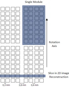
4 × 8 APD arrays (1.6 × 1.6 𝑚𝑚2 pixel size) in a double-readout configuration. This constitutes one module. Each 24 modules are grouped (2 × 12) into one supermodule and each detector head is formed by assembling 4 supermodules side by side, as shown in Figure 3.3. The Clear-PEM scanner consists of two parallel detector heads covering a 17.3 × 15.2 𝑐𝑚2 FOV, coming to a total of 6144 LYSO:Ce crystals [22].
Figure 3.3: Schematic drawing of the Clear-PEM scanner [18].
3.2.2. COINCIDENCE DETECTION
These two heads are designed to detect and localize the origin of the simultaneous back-to-back annihilation photons, also known as coincidences. There are three types of coincidence events that can be measured: true, scattered and random.
Figure 3.4: Types of coincidences detected in a PET imaging system: (a) Scattered coincidences; (b) Random coincidences; (c) True coincidences. Figure adapted from [23].
square of the activity in the patient and becomes more dominant at higher activity levels. The goal in PEM, as well as in PET imaging, is to be able to measure and reconstruct the distribution of true events while minimizing the scattered and random coincidences and correcting for the bias associated with the scattered and random coincidences [23].
The total number of coincident events acquired by a pair of detectors is related to the integral of the activity along the LOR that joins the two detectors. By assessing the integral of the activity along sets of LORs it is possible to obtain projection data that can be reconstructed and form an image of the distribution of radioactivity within the patient [3].
Only a small number of the events processed by each detector are in coincidence. The rate of events processed by each detector is often referred to as the single event rate for that detector, whereas the coincidence event rate includes true events, scattered events and random events. [23]
For some detectors, it is possible to measure the Time-of-Flight (TOF) of the photons: extremely fast scintillators with a good time resolution are used to assess the actual time difference (𝛿𝑡) between the detection of two coincident photons originating from the same annihilation process. Using the speed of light, c, and the precise values of the TOF of the photons, the distance from the annihilation point to each detector will be calculated and thus the exact point of the annihilation in the LOR defined. This method is then used to improve the signal-to-noise ratio (SNR) in image data, resulting in higher image quality,
Chapter 4.
Data Acquisition and Image Reconstruction
This chapter will be used to describe the path that data undergoes since its acquisition by the Clear-PEM detectors until it becomes an image ready for analysis.
During the exam, a number of views are acquired at different positions given by the rotation of the detectors around the breast. Each view, or projection, will only give information about one plane, much like a picture. They all need to be combined and enter a series of procedures that will, in the end, generate a 3D image of the radiotracer’s distribution inside the examined breast.
There is more than one way to transform the projections into a tomographic image, and as each step of the process is explained, all the solutions will be presented, but only the ones selected for this work will be fully explained. In this work, all datasets were rebinned (process which will be explained later) into 2D Lines of Response (LORs) using Single Slice Rebinning (SSRB) and grouped into linograms. For this reason, we will centre our attention on 2D image reconstruction methods.
Originally, all the software used was developed in C. With the development of the project came the need to have specific software designed for image visualization and data analysis, so all the image reconstruction algorithms were optimized to IDL data language [25] and embedded in the visualization software developed.
4.1.
Organization of Acquired Data
The amount of data that emerges from these exams is quite large, requiring organization and parameterization, the first steps of the image reconstruction process.
Throughout the exam, events that meet both the energy and timing criteria are saved to disk in a binary raw data file. After each scanner acquisition, a list-mode file containing relevant information regarding the event, such as the activated crystals, the interaction coordinates (x ,y, z), the deposited energy and a time stamp, is stored sequentially on disk and used directly for image reconstruction [26]. List mode data is advantageous for reconstruction and image correction studies, as the data for reconstruction can be selected from the original file, by creating a new one. Also, it is compact for the big sets of 3D data, and it is easy to convert to quite a few types of parameterization.
After this, a data parameterization will occur, in which the similar LORs will be grouped accordingly to their geometrical characteristics. The most commonly used parameterization in both 2D and 3D whole-body PET scanners, due to their cylindrical shape, is the sinogram [27, 28] – a histogram obtained with polar coordinates. For this kind of systems, the angular parameterization is an obvious choice, because treating each angular projection separately is advantageous for the reconstruction.
As we have seen, the Clear-PEM scanner has two planar detectors that rotate around the breast. For this kind of tomography, called limited angle tomography, the polar coordinates might not be the best choice, but perhaps a set of coordinates based on the planar nature of the acquisition geometry, which would also present advantages for the reconstruction process. Instead of corresponding to a sinusoidal curve, like in a sinogram, the LORs that pass through a fixed point in the object should correspond to a straight line. This kind of parameterization exists, is called linogram [29, 30] and was our choice for this work.
4.1.1. DATA REBINNING
As explained previously, the volume of data that emerges from 3D PET is quite large. In order to make up for the lack of computer power and to improve the reconstruction speed, a procedure called rebinning was created. The objective is to divide the 3D data into smaller 2D data sets. By doing so, instead of reconstructing all the data at the same time, each set will be reconstructed independently, significantly reducing computational time and allowing its use in clinical practice. Although rebinning methods are not specifically a reconstruction procedure, they are an important addition to the group of techniques that bear on three-dimensional image reconstruction problems [23].
transform – Fourier rebinning (FORE) algorithms [33] were presented, more accurate and more time consuming. Eventually, they originated an exact algorithm, with the Fourier transform principle together with some particularities of John’s equation - FORE-J [28, 34, 35].
Although the FORE-J algorithm has been developed for the Clear-PEM scanner, it is yet to be corrected. This work was developed using only SSRB, so it will be presented in detail.
The Single Slice Rebinning (SSRB) algorithm [31] is very fast but leads to inaccurate solutions. Its main goal is to transform each oblique LOR in a LOR perpendicular to the rotation axis lying in the plane that crosses the original LOR in its midpoint [28] (see Figure 4.1). This method is accurate for sources near the scanner axis, since the rebinned LOR will still cross the emission point. Nevertheless, axial blurring and transaxial distortions increase with the distance from the axis of the scanner, and, at the same time, spatial resolution gets degraded.
Figure 4.1: Single Slice Rebinning.
4.1.2. LINOGRAMS
In 1987, Edholm [29] proposed an alternative to the highly used sinogram by choosing new coordinates (𝑢,𝑣) to parameterize a LOR in limited angle tomography acquisitions. The linogram will be a plot of 𝑣 as a function of 𝑢, with this coordinates defined by:
2
1
2 d
d x
x
u Eq. 4.1
2
1
2 d
d x
x
v Eq. 4.2
According to these definitions, in a linogram, each column, 𝑢, represents the interception coordinate between the LOR and the central plane of the FOV, and each line, 𝑣, is a function of the LOR’s slope (see Figure 4.2).
Figure 4.2: Definition of linogram coordinates. Figure adapted from [28].
Each line in a linogram represents a set of LORs that cross a certain pixel (x0, y0),
which means that they have to satisfy the following condition:
𝑢= 𝑥+𝑦𝑣 [29] Eq. 4.3
as proven in the example shown on Figure 4.3. Here one can see that for five activity sources, five straight lines are generated.
Figure 4.3: Linogram example. Figure adapted from [28].
The backprojection (see section 4.3) of all the LORs passing through a point in the image now corresponds to integration along a straight line in the linogram, which is a simpler interpolation problem than the used backprojection of sinograms [23].
Usually, for cylindrical detectors, sinograms and linograms are represented as a 2D rectangular map. As a result of the well defined FOV of the detector, it is easy to understand the limits of the LORs acquisitions and determinate the shape of the detectable region. For LORs perpendicular to the detector (𝑣= 0), all possible 𝑢 values correspond to detectable LORs (Figure 4.4 (a)), whereas for LORs with the maximum slope (𝑣𝑚𝑎𝑥 or 𝑣𝑚𝑖𝑛) only LORs with 𝑢= 𝑢𝑚𝑒𝑑𝑖𝑢𝑚 are detectable (Figure 4.4 (b)). Also LORs crossing the central plane of the FOV in its limits (𝑢𝑚𝑎𝑥 or 𝑢𝑚𝑖𝑛) are detectable only with 𝑣 = 0 (Figure 4.4 (c)). Thus, all the detectable LORs are located within a rhombus (Figure 4.4 (d)), whose dimensions depend on the distance between the detectors [28].
Figure 4.4: (a) Detectable LORs with v=0; (b) Detectable LORs with v=vminand v=vmax; (c) Detectable LORs with
u=umin and u=umax; (d) Detectable region of a linogram. Figure adapted from [28].
A generalization of the 2D linogram was presented in 2001 by Kinahan et al [36], introducing the concept of the planogram data format for fully-3D imaging.
4.2.
Image Reconstruction
The purpose of tomographic image reconstruction is to take the data acquired by the scanner as projection views and transform it into an accurate three-dimensional
representation of the patient, or in PEM’s case, of the radiopharmaceutical distribution in
4.3.
Analytic Image Reconstruction
The basis for most analytic reconstruction methods is linear superposition of backprojections, often known simply as backprojection. This algorithm is based on the mathematics of computed tomography (CT) that relates line integral measurements to the activity distribution in the object. Essentially, the counts from a detector pair are being projected back along the line from which they were originated. This process is repeated for all valid detector pairs in the PET system, and all the counts from all detector pairs are added, as schematized on Figure 4.5.
Figure 4.5: Backprojection. The image reconstruction quality increases with the number of projections [23].
The most frequently used method is the Filtered Backprojection (FBP) [15, 23, 37]. Not only it is fast, but intuitive and has a well known performance, thus becoming appealing for clinical practice. However, it has some downsides. The biggest one comes from the fact that we do not have continuous sampling of the object, but a finite number of projections, and as a result, a radial blurring effect is generated. Moreover, the impossibility of incorporating previous knowledge such as the structures in study, the geometry of the detector or even a model of emission into the algorithm, are some of the reasons that encourage the use of iterative methods instead.
4.4.
Iterative Image Reconstruction
Due to long computational time, iterative image reconstruction methods [38] were pushed aside from clinical practice for years. Only more recently, with the enhancement of computer power, have these methods experienced significant progress, becoming faster and a valid option for clinical tomographic reconstruction.
The main goal of this method is to generate a close estimate of the distribution of the activity in the different planes of the image and to compare the projections of this estimate with the projections acquired. The algorithm starts with an initial estimate of the data to produce a set of transaxial slices. These slices are then used to create a second set of projection views, which are compared to the original ones acquired from the patient. The
between, or ratio of, the two sets of projection views. If everything proceeds efficiently, each sequence, or iteration, generates a new set of projection views that is more similar to the original ones. The process is complete when the difference between the projection views of the estimated data and the original data is below a pre-determined threshold [17].
Even though the final results take longer to achieve than in analytic methods, the estimates are progressively more accurate and, consequently, much closer to the real activity in the object. Furthermore, in the backprojection method, the value of one projection is assumed to be the integral along the respective LOR, forcing all the corrections to be applied before the reconstruction. As for the iterative methods, there is the possibility of applying corrections to the data during the reconstruction, or even incorporating anatomical information from previous MRI or CT studies of the patient [39]. Every iterative method follows the scheme on Figure 4.6.
Figure 4.6: Iterative reconstruction process. Figure adapted from [23].
For the Clear-PEM scanner, three different 2D iterative image reconstruction algorithms have been applied: one algebraic – the Algebraic Reconstruction Technique (ART), and two statistical algorithms – the Maximum Likelihood - Expectation Maximization (ML-EM) and the Ordered Subsets - Expectation Maximization (OS-EM). For this work, only the OS-EM was used.
According to Fessler [40] the image reconstruction methods have five components:
1. a finite parameterization of the positron-annihilation distribution, i.e., the measurements taken (𝒀);
2. a system matrix (𝑨) – a model of the emission and detection process that relates the activity distribution inside the organ (𝒇) with the measurements taken (𝒀), for example:
3. a statistical model for how the detector measurements vary around their expectations;
4. an objective function that is to be maximized to find the image estimate;
5. an algorithm, typically iterative, for maximizing the objective function, including specification of the initial estimate and stopping criterion.
Accordingly, for every iterative image reconstruction, the calculation of a system matrix 𝑨is required. Each element of 𝑨(denoted by 𝑎𝑖𝑗) represents the contribution of the voxel 𝑗 (element of 𝒇) in the object to the bin 𝑖 (element of 𝒀) in the projection, or, simplifying, each element of the matrix 𝑎𝑖𝑗 defines the probability of the emitted photons in a certain voxel 𝑗 had originated a certain LOR 𝑖.It is in the specification of 𝑨that the model of the projection process can become as simple or as complex as we require, because the intensity of a projection bin is a weighted sum of intensities of the image voxels [23].
4.4.1.
SYSTEM MATRIX CALCULATIONThe system matrix represents the physics and the geometry of the emission and detection processes, for that particular system. Hence, when the scanner has a fixed geometry, the system matrix may be calculated only once and stored to be used in all image reconstructions required. However, when the system of detection has a variable geometry, the system matrix must be recalculated every time the geometry is changed.
Independently of the method used to calculate the system matrix, at the end of the calculation, the probabilities need to be normalized. This normalization guarantees that the sum of the probabilities that corresponds to a certain coincidence is always equal to one if the LOR is detectable, or equal to zero if it is undetectable.
There were three methods used in this scanner: the pixel-driven, the ray-driven and the tube-driven method. Only the latter was used for this work, but a small presentation of all three will be made to make comprehension easier. This is a review of the work of Nuno Matela in [28].
4.4.1.1. The Pixel-Driven Method
In this method, each element of the system matrix is determined by the analysis of which LORs can be originated from each pixel. The 𝑣 coordinate of all detectable LORs that cross a certain pixel 𝑗 is calculated. Note that only the values of 𝑣 within the limits of the detector plates will be considered. For each pair (𝑗, 𝑣) the value of 𝑢 is determined with:
0 0
2
y z
z z v
u
where 𝑦0 and 𝑧0 are the pixel 𝑗 coordinates and 𝛥𝑧 is the distance between the detector
plates. Because the result of this equation is a real value of 𝑢, which does not always match the centre of the linogram bin, a correction is made by dividing the probability of occurring a LOR with a given direction, generated in this pixel, by the two nearest bins of 𝑢, taking into account the distance between the centre of each bin and the intersection coordinate. This distance returns an indication of how close 𝑢 is from the centre of the two nearest bins.
4.4.1.2.The Ray-Driven Method
Opposite to the previous method, in the ray-driven method every LOR is analysed to determine from which pixel it could have been originated.
Based on the Siddon method [41], each element of the matrix is defined as the length of the segment of the LOR 𝑖 inside pixel 𝑗. Firstly, the coordinates of the intersections between the LOR 𝑖 and the vertical lines of the pixel lattice are determined analytically in
LOR units (defined as fractions of the LOR’s total length), and then arranged as a vector 𝛼 𝑦. The procedure is repeated with the horizontal lines of the lattice, and the vector 𝛼 𝑧 is created. The following step is the merge of the two vectors, where all the coordinates are sorted. The difference between two consecutive coordinates is calculated and the vector 𝛼 created.
The component 𝛼𝑗 of this vector is defined as the probability that the LOR had been originated in a certain pixel that can be localized in the FOV by the coordinates 𝑚𝑗 and 𝑛𝑗, calculated using the following equations and where 𝑦1 is the coordinate in the lower detector. d y y m j j j 2 1 1 Eq. 4.6
d znj j j
2
1
Eq. 4.7
The procedure is repeated for all possible LORs and the results presented as a matrix.
4.4.1.3.The Tube-Driven Method
length of the several segments, the 𝑎𝑖𝑗 elements are determined by the exact calculation of the area of intersection between each TOR 𝑖 and each pixel 𝑗. The area is calculated using the same procedure presented for the ray-driven method, but now only applied to the left limit of the tube, 𝐿, which has a base with the same width of the pixels. From this, there are only three possible types of intersection: a trapezium (Figure 4.7(a)), the entire pixel except one or two triangles (Figure 4.7(b)) or only one triangle (Figure 4.7(c)).
Figure 4.7: Possible intersections between a TOR and a pixel: (a) a trapezium, (b) the entire pixel except one or two triangles, or (c) one triangle.
For the exact calculations of the interaction areas involved in each case, Eq. 4.8, Eq. 4.9 and Eq. 4.10 should be used.
sin 2 2 sin , ) ( D l h h D
Aa tub Eq. 4.8
2 sin 2 , 2 2 2 ) ( D f h DAb Eq. 4.9
2 sin , 2 D l f DAc tub Eq. 4.10
In these equations, 𝐴 𝐷,𝜃 is the value of the area of intersection between the TOR and the pixel, 𝐷 is the distance between the centre of the pixel and the central line of the TOR, 𝑙𝑡𝑢𝑏 is the length of the base of the TOR, is the size of the pixel, 𝜃 is the angle between the TOR and an horizontal line and 𝑓 𝜃 is defined by Eq. 4.11.
2 4 cos 2
2h ltub
f
Eq. 4.11
Figure 4.8: Variables used to calculate the area of intersection between the TOR and the pixel.
In all approaches probabilities were normalized to one for each value of j.
4.4.2.
THE ALGEBRAIC RECONSTRUCTION TECHNIQUE (ART)In our image model (𝒀𝒊 =𝑨𝒊𝒇), each measurement, 𝑌𝑖, a function of the activity distribution, is a hyperplane where the solution of 𝑓 must lie. There are as many hyperplanes as projections and the solution of 𝑓 must belong simultaneously to all, which means the solution will lie in the intersection of all hyperplanes. Still, this assumption will only be valid for noiseless data. Noise can be defined as random, unwanted signal that interferes with the processing or measurements of the desired signal [23].
When noise is present in the acquired data, the assumption that all hyperplanes intercept themselves in a single point is generally not true since each hyperplane will be slightly shifted from its original position. In this situation, we will probably have multiple intersections corresponding to partial solutions, i.e., solutions that satisfy part of the constraints but not all of them. This will introduce a problem to the iterative algorithm since it will not converge to a unique solution, switching cyclically between partial solutions. This problem is solved by the introduction of a relaxation parameter (𝜆) [28].
The algebraic reconstruction technique, or ART, was applied to medical image reconstruction for the first time by Herman [42], and is one of the possible methods to determine the intersection point of all hyperplanes.
In the ART algorithm to determine fj, a linogram of an estimate is calculated and a subset (𝑌𝑖) of the estimation linograms is compared with the corresponding subset obtained from the measurements by calculating the algebraic difference. In each ART sub-iteration, the activity is updated in order to minimize the difference between these two sets [43].
ij l il l k l il i k k j k j a a f a Y f f
2 11 Eq. 4.12
Or, in words, the 𝑎𝑖𝑗 is the model of emission and detection that corresponds to the probability that a detection 𝑌𝑖 had been originated in pixel 𝑗. The relaxation parameter must have a value between 0 and 1, in order to keep the result between the different hyperplanes. By doing so, an underrelaxation of the method will be applied, limiting the update process, which prevents the algorithm from entering in a loop.
High values of the relaxation coefficient, λ, allow fast convergence speed but also noisy reconstruction images, and on the contrary, low values allow smoother images but lower convergence speed. The choice of which to optimize is always made.
4.4.3.
THE MAXIMUM LIKELIHOOD -EXPECTATION MAXIMIZATION (ML-EM)The maximum likelihood – expectation maximization (ML-EM), developed by Dempster [44] and applied for image reconstruction for emission tomography by Shepp and Vardi [45], is often considered the source of the best image reconstruction algorithms. It is an iterative statistical algorithm based on the fact that the best model for the physics involved in the emission and detection of radioactive decay processes is the Poisson distribution.
Following the same principle as ART, the acquired data will be represented on a vector 𝑌, whose element 𝑌𝑖 represents the number of coincidences detected along the direction defined by the LOR 𝑖. The number of photon pairs emitted in each voxel 𝑗 is given by 𝑓𝑗.
The main idea of the ML-EM algorithm is to maximize a likelihood2 function, which can be achieved using:
i j k j ij i ij i j i k j k j f a Y a a f f ' 1 ' ' ' ' 1 Eq. 4.13Nevertheless, this method has two major drawbacks: very slow convergence and it is unstable in the presence of noisy data.
4.4.4.
THE ORDERED SUBSETS -EXPECTATION MAXIMIZATION (OS-EM)The ordered subsets – expectation maximization (OS-EM) is usually understood as an accelerated version of ML-EM. Proposed by Hudson and Larkin [46], instead of using
2
Likelihood is a general statistical measure that is maximized when the difference between the
simultaneously all values of 𝑌𝑖 to update a new estimation of the activity distribution, the elements of the linogram are divided into subsets. Each reconstructed image update is then performed using only one subset (one sub-iteration)[43]. The process can be described by:
k S i k j ij i ij k S i j i k j k j f a Y a a f f 1 ' ' ' ' 1 Eq. 4.14where 𝑆(𝑘) is the subset to be used in kth image update.
One OS-EM iteration, composed of n sub-iterations, takes approximately the same time as to iterate ML-EM once, yet it consists in n times more updates of the estimated activity distribution.
![Figure 2.4: Predominant type of interaction for various combinations of incident photons and absorber atomic numbers [17]](https://thumb-eu.123doks.com/thumbv2/123dok_br/16535725.736524/30.892.244.619.83.373/figure-predominant-interaction-various-combinations-incident-photons-absorber.webp)