SIDNEY ROSA VIEIRA (2); JOSÉ RUY PORTO DE CARVALHO (3); ANTONIO PAZ GONZÁLEZ (4)
ABSTRACT
The semivariogram function fitting is the most important aspect of geostatistics and because of this the model chosen must be validated. Jack knifing may be one the most efficient ways for this validation purpose. The objective of this study was to show the use of the jack knifing technique to validate geostatistical hypothesis and semivariogram models. For that purpose, topographical heights data obtained from six distinct field scales and sampling densities were analyzed. Because the topographical data showed very strong trend for all fields as it was verified by the absence of a sill in the experimental semivariograms, the trend was removed with a trend surface fitted by minimum square deviation. Semivariogram models were fitted with different techniques and the results of the jack knifing with them were compared. The jack knifing parameters analyzed were the intercept, slope and correlation coefficient between measured and estimated values, and the mean and variance of the errors calculated by the difference between measured and estimated values, divided by the square root of the estimation variances. The ideal numbers of neighbors used in each estimation was also studied using the jack knifing procedure. The jack knifing results were useful in the judgment of the adequate models fitted independent of the scale and sampling densities. It was concluded that the manual fitted semivariogram models produced better jack knifing parameters because the user has the freedom to choose a better fit in distinct regions of the semivariogram.
Key words: Semivariograms, stationarity, topography, scale of variation.
RESUMO
JACK KNIFING PARA VALIDAÇÃO DE SEMIVARIOGRAMAS
A função de ajuste do semivariograma é o aspecto mais importante da geoestatística, por esse motivo, o modelo escolhido deve ser validado. Jack knifing pode ser um dos métodos mais eficientes para esta finalidade. O objetivo deste estudo foi mostrar o uso da técnica jack knifing para validar modelos de hipótese geoestatística e de semivariograma. Para essa finalidade, foram analisados dados topográficos de seis campos de escalas distintas e de diferentes densidades de amostragem. Devido aos dados topográficos selecionados terem apresentado tendência em todos os campos, fato verificado pela ausência de patamar no semivariograma, a tendência foi removida através do ajuste de uma superfície de tendência pelo método dos quadrados mínimos. Os modelos de semivariograma foram ajustados por diferentes técnicas e validados pela comparação dos resultados do jack knifing. Os parâmetros de Jack knifing analisados foram a interseção, o coeficiente angular e o coeficiente de correlação para a regressão linear entre valores estimados e medidos, e a média e a variância dos erros calculados pela diferença entre valores medidos e estimados divididos pela raiz quadrada da variância da estimativa. Os resultados do jack knifing foram úteis no julgamento adequado dos modelos ajustados aos semivariogramas, independentemente da escala e da densidade de amostragem. Conclui-se que os modelos de semivariograma ajustados manualmente resultaram em melhores parâmetros de jack knifing devido à liberdade de escolha, por parte do usuário, do melhor ajuste em regiões distintas do semivariograma.
Palavras-chave: erro reduzido, estacionaridade, topografia, variação de escala.
(1) Received for publication in September 15, 2008 and accepted in March 9, 2010.
(2) Centro de Pesquisa e Desenvolvimento de Solos e Recursos Ambientais, Caixa Postal 28, 13001-970, Campinas (SP). Email: [email protected].
(*) Corresponding author.
(3) EMBRAPA/CNPTIA, Campinas, (SP).
1. INTRODUCTION
Soil variability has always existed and if not taken into account when field work is involved, there is a risk to make wrong conclusions out of the data. If the soil variability is somewhat organized in the space and spatial dependence can be determined, the data must be analyzed using geostatistics. In this condition, it is possible to estimate values for the unsampled locations without bias and with minimum variance through the kriging interpolation technique. On the other hand, in order to make appropriate use of geostatistics, it is necessary assume that the measured data correspond to one realization of a continuous random function which exists in every point in the field (Vieira et al., 1983). For this reason, it is necessary that the data fit into some stationarity hypothesis (Vieira, 2000). Besides, the experimental semivariogram calculated will be a series of discrete data pairs of distances and semivariances to which a continuous mathematical function must be fitted. For this reason, it is commonly said that semivariogram function fitting is the most important aspect of geostatistics (McBratney and
WeBster, 1986) and the model chosen must be validated. Methods for fitting a model to the semivariogram are well documented in the literature (Wollenhauptet al.,
1997; GotWay, 1991; lee, 1994; carValho and Vieira,
2004). Jack knifing may be one the most efficient ways
for this validation purpose (Vieiraet al., 1983). Through this technique, a measured value is temporarily taken out of the data set, and then it is estimated using the semivariogram model fitted. Simultaneously with the estimated value, the estimation variance is also calculated in the kriging procedure. This procedure is successively repeated for every measured value and at the end it is possible to calculate errors using measured, estimated and estimation variance values whose values must remain within some specified statistical limits. This technique is also known as a cross validation or “leave-one-out” and has been used in some different applications (schechtMan and WanG, 2004; Fortes et al., 2004; Zhu et al., 2008, Mello et al., 2008, pires and strieder, 2006). The objective of this study was to show the use of the jack knifing technique to validate geostatistical hypothesis and semivariogram models.
2. MATERIAL AND METHODS
Data
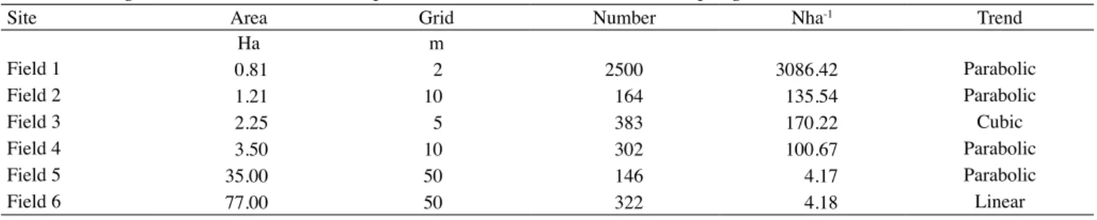
The following data sets used were: 1) A square field of 90m on each side named FIELD 1 sampled on a 2m grid with a total of 2500 points; 2) A triangular field named FIELD 2 of 110m by 220m, sampled on a 10m square grid, with a total of 164 points; 3) An approximately rectangular field named FIELD 3 measuring 90x250m, sampled on trapezoidal grid of 5m, with a total of 383 points; 4) An approximately rectangular field named FIELD 4, measuring 120x160m sampled on a 10m square grid with 302 data points; 5) An approximately rectangular field named FIELD 5, of approximately 35ha, sampled on a 50m square grid in a total of 146 data points; 6) A circular field named FIELD 6 of 77ha sampled on a square grid of 50m, at every one of the 322 points.
A summary about the six fields with grid information is shown in table 1. Topography was chosen as a data set to be analyzed because its form is easily verified in the field and its surface does not change with time allowing for the field validation of the results if necessary. These specific fields were chosen because they represent a very wide range of scales (from 0.81 to 77 hectares), of grid sampling spacing (from 2 to 50 m), of number of values (from 2500 to 146 values) and consequently of number of samples per hectare (from 3086.42 to 4.17). Because the topographical data showed very strong trend for all fields as it was verified by the absence of a sill in the experimental semivariograms, the trend was removed with a trend surface fitted by the minimum square deviation, according to Vieira
(2000). The degree of the trend surface used in each case
is listed in the last column of table 1.
Detrending
The trend removal technique used is described in Vieira (2000). The presence of a trend is detected when the semivariogram does not have a stable sill. This condition violates the intrinsic hypothesis as it represents a field for which the mean value depends on the spatial position. The simplest trend removal consists in fitting a three dimensional surface to the data
Table 1. Area, grid, number, number of sample (N ha-1) and trend removed to sampling sites field 1 until 6
Site Area Grid Number Nha-1 Trend
Ha m
Field 1 0.81 2 2500 3086.42 Parabolic
Field 2 1.21 10 164 135.54 Parabolic
Field 3 2.25 5 383 170.22 Cubic
Field 4 3.50 10 302 100.67 Parabolic
Field 5 35.00 50 146 4.17 Parabolic
by the least squares and subtracting its values from the originals. For a parabolic trend surface, the equation is
(1) where Z*(x,y) is the estimated trend surface, X
and Y are the coordinate positions and A0, A1, A2, A4,
A4 and A5 are the regression parameters determined by
the least squares method. This surface is then subtracted from the originals generating a new variable which may be called Residuals.
(2)
The criteria for the choice of the degree for the detrending surface is the simplest surface that will produce a semivariogram with a stable sill. Thus, if a linear surface solves the starionarity problem producing a semivariogram with a sill, there no need to look for any other degree of a surface.
Semivariogram
The semivariogram is, by definition:
(3) And can be estimated by:
(4)
where N(h) is the number of pairs of measured values Z(xi), Z(xi+h), separated by a vector h (Journel and huiJBreGts, 1978). The graph of γ*(h) versus the corresponding values of h, called semivariogram, is a function of the vector h, and therefore it depends on both magnitude and direction of h. When the semivariogram is the same for all directions it is called isotropic. Many variables show anisotropic semivariograms depending on the dimensions of the field and of the nature of the variability. There are ways of transforming an anisotropic semivariogram (Journel and huiJBreGts,
1978; BurGessand WeBster, 1980) in order to reflect the
variability in different directions. Jack knifing procedure can also be used to verify the distance range over which a semivariogram can be used before anisotropic effects may affect the results (Vieira, 2000).
Models
Experimental semivariograms contain a set of discrete data points of distance and semivariance. A model must be fit to the experimental data with the objective of having semivariances available for every distance needed (GotWay, 1991). In order to be used to properly describe the spatial variability of any variable,
one of the requirements on the model is that the function used must be conditional positive definite (McBratney and WeBster, 1986). This condition will guarantee that the variances calculated will be positive. The main models which satisfy that condition and are adequate for use in geostatistical calculations are the spherical, the exponential and the Gaussian. On the equations bellow, C0, C1, and a represent the nugget effect, the structural variance and the range, respectively.
For the spherical model, usually symbolized as Sph(C0, C1, a), the equation is:
(5)
The exponential model, symbolized as Exp(C0,
C1, a), the equation is:
(6)
The gaussian model, symbolized as Gau(C0, C1,
a), the equation is:
(7)
With the parameters fitted to the semivariogram the dependence ratio (DR) can be calculated (ZiMBack, 2001)
(8)
The dependence ratio (DR) represents the proportion of the semivariance which is structured. The smallest the DR value the weakest is the spatial dependence.
Jack knifing
estimated and estimation variances through which it is possible to calculate error parameters whose values must be within some statistically known limits. More details about the process can be found in Journeland huiJBreGts
(1978). There are some reports in the literature with some
applications of the cross validation technique but using only the one-to-one graph of measured versus estimated values (Forteset al., 2004; Melloet al., 2005; Melloet al.,
2008). In this paper, six different jack knifing parameters
are examined as criteria for judging the performance of semivariogram models, neighborhood of estimation and geostatistical hypothesis. All the estimations were made using ordinary kriging interpolation technique.
The one-to-one Measured vs Estimated values
Using the N measured values, Z(xi), and the N values estimated through the jack knifing procedure, Z*(xi), it is possible to make the graph known as the one-to-one and to calculate the linear regression between measured and estimated values. The regression will be:
(9)
Where a is the intercept, b is the slope and r2 is the
coefficient of determination between Z*(xi) and Z(xi). Thus, if the estimation, Z*(xi), is identical to the measured, Z(xi), for every one of the N points, then a is zero (0), b and r2 are equal to one (1.0), and the graph of
Z(xi) vs Z*(xi) would be a series of points on the one-to-one line. As the value of a depart from zero (0) to positive values, it is an indication that the estimator Z*(xi) is over estimating small values of Z(xi) and under estimating large values. As the value of a gets negative the reverse happens. This way, the quality of the estimation may be assessed judging these parameters. The examination of the one-to-one scatter plot of measured versus estimated values is an important aid in judging the estimation performance but it only makes sense for the best selection of the other parameters (Vieiraet al., 1983). Therefore, it is an useful technique but it needs the other parameters before a decision on neighborhood size and semivariogram parameters ca be made.
The reduced error
Remembering that through the kriging estimation of values, Z*(xi), there is always a value of the estimation variance, σ2
k(xi), corresponding to the uncertainty of the
estimation process (Vieiraet al., 1983), then it is possible to define the reduced error as:
(10)
The division by the square root of the estimation variance causes the reduced error, RE(xi),
to be dimensionless which is a convenient situation for comparison between different variables.
The unbiasedness condition of kriging estimation requires that:
(11) The minimum variance condition requires that:
(12)
These properties make this kind of error assessment a very valuable and easy to use tool for validation of geostatistical procedures. Because these errors have fixed reference values of 0 (zero) and 1 (one), respectively, and are dimensionless, their judgment and interpretation is much easier and allows comparison with other variables expressed in different units.
The root mean square error (RMSE)
Another very powerful parameter of the jack knifing technique is the RMSE which can be calculated using
2
(13)
The disadvantage of this kind of error is that it does not have any standard to be compared with. Therefore the best results of the jack knifing technique will be obtained when the RMSE is minimum.
3. RESULTS AND DISCUSSION
A summary about the data and the places from where they were sampled is shown in table 1, where it can be seen that the areas sampled range from 0.81 ha to 77 ha, and the sampling densities range from 3086 to 4.18 samples ha-1. Therefore, the areas sampled represent
a very large range of field dimensions and topographic conditions, and for these reasons we hope that the results are adequate to evaluate the performance of the proposed method of validation. All the data sets presented very strong trends which had to be removed in order to satisfy the intrinsic hypothesis. The trend was removed by fitting with least square method a tri dimensional surface and subtracting it from the original data as described for
the linear already did it. As shown in the last column of table 1, from the six fields studied, for one a cubic trend surface was used, for four the parabolic surface and for one the linear surface.
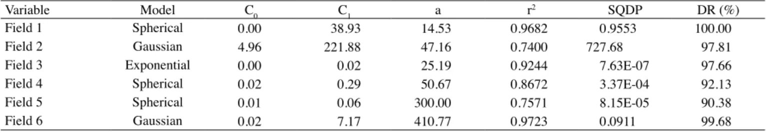
The parameters for the models fitted to the semivariograms are shown in Table 2 and the corresponding graphs of the semivariograms are shown in Figure 1 with the models fitted. It can be seen that
Table 2. Parameters of the models fitted to the semivariograms, nugget effect (Co, structural variance (C1), range (a), coefficient of determination (r2), sum of squares deviation weighed (SQDP) and dependence ratio (DR%) to sampling sites field 1 until 6
Variable Model C0 C1 a r2 SQDP DR (%)
Field 1 Spherical 0.00 38.93 14.53 0.9682 0.9553 100.00
Field 2 Gaussian 4.96 221.88 47.16 0.7400 727.68 97.81
Field 3 Exponential 0.00 0.02 25.19 0.9244 7.63E-07 97.66
Field 4 Spherical 0.02 0.29 50.67 0.8672 3.37E-04 92.13
Field 5 Spherical 0.01 0.06 300.00 0.7571 8.15E-05 90.38
Field 6 Gaussian 0.02 7.17 410.77 0.9723 0.0911 99.68
0 5 10 15 20 25 30 35 40 45
0 10 20 30 40 50 60
S e m iv a ri a n c e Distance (m) (a) Field 1 0.81ha
Elevation Parabolic Residuals
Sph(0,38.93,14.53) 0 50 100 150 200 250 300 350
0 20 40 60 80 100
S e m iv a ri a n c e Distance (m) (b) Field 2 1.21 ha
Elevation Parabolic Residuals Gau(4.96,221.88,47.16) 0.000 0.002 0.004 0.006 0.008 0.010 0.012 0.014 0.016 0.018 0.020
0 20 40 60 80 100
S e m iv a ri a n c e Distance (m) (c) Field 3 2.25 ha
Elevation Cubical Residuals
Exp(0.00037,0.016,25.19) 0.00 0.05 0.10 0.15 0.20 0.25 0.30 0.35 0.40
0 20 40 60 80 100
S e m iv a ri a n c e Distance (m) (d) Field 2 3ha
Elevation Parabolic Residuals
Sph( 0.025, 0.292, 50.67)
0.00 0.01 0.02 0.03 0.04 0.05 0.06 0.07 0.08 0.09 0.10
0 50 100 150 200 250 300 350 400
S e m iv a ri a n c e Distance (m) (e) Field 5 35ha
Elevation Parabolical Residuals Sph( 0.06, 0.058, 300)
0 1 2 3 4 5 6 7 8 9
0 100 200 300 400 500 600 700 800
S e m iv a ri a n c e Distance (m) (f) Field 6 77 ha
Elevation Linear Residuals
Gau(0.023,7.17,410.77)
all semivariograms fit the intrinsic hypothesis (they all have a very well defined sill) and that the worst fitting found was for field 2, with r2 = 0.7400. Otherwise, in
general, the models fit quite well the experimental semivariograms. The dependence ratio shown in the last column of Table 2 indicates the very high degree of continuity that the residuals for the topographical data has. From semivariograms for the six fields, three of them were fitted to the spherical model, two to Gaussian and one to exponential model. Notice that the r2 values for the models fitted to the semivariograms
(Table 2) are the lowest for field 2 and field 5 caused by the dispersion of values around the sill. Not much
importance should be given to this fact as the main portion of the semivariogram is the short distance (McBratneyand WeBster, 1986). On the other hand, all semivariograms are very well fitted to their respective models for the distances smaller than the range.
The results of jack knifing for the five parameters (a, b, and r2 for the regression 1:1, mean and variance of the
reduced errors) used is shown in figure 2. The intercept values (Figure 2a) indicate that the semivariograms for all six surfaces produced good regression between measured and estimated values, as all of them, except for field 2 with four neighbors, approach a zero intercept. The slope
-0.30 -0.25 -0.20 -0.15 -0.10 -0.05 0.00 0.05 0.10
0 10 20 30 40 50
In
te
rc
e
p
t Number of Neighbors
(a)
Field 1 Field 2 Field 3
Field 4 Field 5 Field 6
0.8 0.9 1.0 1.1 1.2
0 10 20 30 40 50
S
lo
p
e
Number of Neighbors
(b) 0.6 0.7 0.8 0.9 1.0 1.1 1.2
0 10 20 30 40 50
C o e ff ic ie n t o f D e te rm in a ti o n
Number of Neighbors
(c) -0.25 -0.20 -0.15 -0.10 -0.05 0.00 0.05 0.10 0.15
0 10 20 30 40 50
M e a n E rr o r
Number of Neighbors
(d) 0.0 0.2 0.4 0.6 0.8 1.0 1.2 1.4 1.6 1.8 2.0
0 10 20 30 40 50
V a ri a n c e o f E rr o r
Number of Neighbors
(e) 0.0 0.5 1.0 1.5 2.0 2.5 3.0 3.5 4.0 4.5 5.0
0 10 20 30 40 50
R
M
S
E
Number of Neighbors
(f)
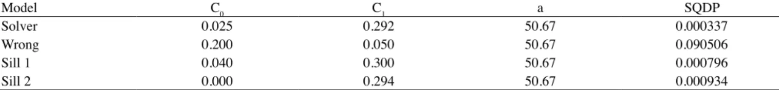
Table 3. Parameter of models fitted (solver, wrong, sill1 and sill2) for jack knifing comparison, nugget effect (Co), structural variance (C1), range (a) and sum of squares deviation weighed (SQDP)
Model C0 C1 a SQDP
Solver 0.025 0.292 50.67 0.000337
Wrong 0.200 0.050 50.67 0.090506
Sill 1 0.040 0.300 50.67 0.000796
Sill 2 0.000 0.294 50.67 0.000934
Table 4. Jack knifing parameters for Field 1, using 20 neighbors
Parameter Result
Number of neighbors 20
Intercept 0.0014
Slope 0.8661
r 0.9384
Mean error 0.0006
Variance 0.7661
Distance 9
of the regression line between measured and estimated values (Figure 2b) approaches the ideal situation (a=1) for any neighborhood above 16 neighbors for all data sets. Field 4 was the only one for which this parameter was separated from the others and the cause for this has not been identified. The coefficients of determination (Figure 2c) showed a wide spread of values. In general, the values for this parameter approach the ideal value of 1.0, except for fields 3 and 5 which presented values around 0.7. The mean error (Figure 2d), except for field 6, are grouped around the ideal value of 0 (zero). The reason for the departure of the mean value for the reduced errors for field 6 is not known at this point. However, for 16 neighbors, all fields have a value of mean error very close to 0 (zero). The variance of the reduced errors (Figure 2e) should ideally approach the value of 1.0. In general all fields present values below 1.0 for the variance of the reduced errors, except for field 2 which presented values much above that level. Figure 2f shows a graph of the Root Mean Square Error (RMSE) between the measured and the estimated values. This parameter, although very robust, its values are somewhat arbitrary because it does not have any standards or ideal value to be compared with. An overall examination of the values of all parameters together shows that most of them approach the ideal values if a neighborhood of 16 values is used as it has been indicated by Vieiraet al. (1983). The square grid sampling may the explanation for this apparent coincidence around 16 neighbors for all of the data sets.
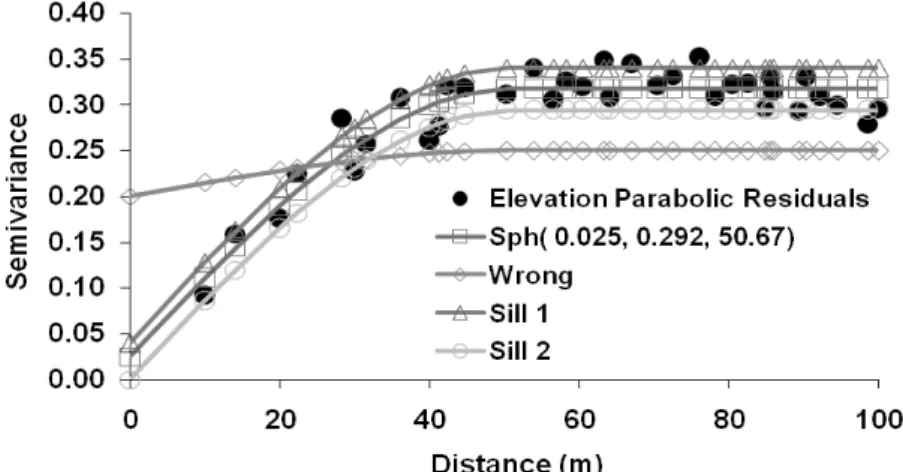
In order to investigate further the jackknifing potential for the validation of semivariogram models, four different models were fitted to the semivariogram for field 5 by different methods. The parameters fitted are shown in table 3 and on graph on figure 3. The four models were named Solver, Wrong, Sill 1 and Sill 2. The model Solver was fitted using the Solver technique in Excel to maximize the coefficient of determination. The
model called Wrong was purposely fitted with a wrong nugget effect value. The models Sill 1 and Sill 2 were fitted by trial and error by manually placing the sill value in different positions in order to provide information about the effect of the proper choice of the sill value on the jack knifing parameters. The results from the jack knifing for these models are shown in figure 4. The results indicate that if one single model had to be chosen it should be the model identified as Sill 2 with 16 neighbors as all the jack knifing parameters approach the ideal values with this choice. It can be clearly seen that the model identified as “wrong” had a very poor performance for all the jack knifing parameters. The above discussion illustrates the idea of using the jack knifing technique for fine tuning the semivariogram model fitting.
Because the data from field 1 was the one with the highest number (2500) and it was also the smallest field (highest density of samples, see Table 1) one set of jack knifing was calculated for this data set with 20 neighbors. The jack knifing parameters are shown in table 4. Except for the variance of the errors, all other parameters are very close to the ideal values. A graph with the measured versus estimated values for this calculation is plotted in figure 5 where it can be seen that there was a very good agreement between measured and estimated values.
4. CONCLUSION
Figure 3. Models fitted to semivariogram of topographic data from FIELD 2.
-0.010 -0.008 -0.006 -0.004 -0.002 0.000 0.002 0.004
0 5 10 15 20 25 30 35 40 45
In
te
rc
e
p
t
Number of Neighbors
(a)
Solver Wrong Sill 1 Siil 2
1.0 1.1 1.2 1.3 1.4 1.5
0 5 10 15 20 25 30 35 40 45
S
lo
p
e
Number of Neighbors
(b)
0.74 0.76 0.78 0.80 0.82 0.84 0.86 0.88 0.90 0.92
0 5 10 15 20 25 30 35 40 45
C
o
e
f.
o
f
D
e
te
rm
in
a
ti
o
n
Number of Neighbors
(c)
-0.006 -0.004 -0.002 0.000 0.002 0.004 0.006 0.008 0.010 0.012 0.014
0 5 10 15 20 25 30 35 40 45
M
e
a
n
E
rr
o
rs
Number of Neighbors
(d)
0.0 0.1 0.2 0.3 0.4 0.5 0.6 0.7 0.8 0.9 1.0
0 5 10 15 20 25 30 35 40 45
V
a
ri
a
n
c
e
o
f
E
rr
o
rs
Number of Neighbors
(e)
R2 = 0.9384
-40 -30 -20 -10 0 10 20 30
-40 -30 -20 -10 0 10 20 30
Measured
E
s
ti
m
a
te
d
Figure 5. One-to-one graph for measured versus estimated values of elevation parabolic residuals for field 1 with jack knifing using 20 neighbors.
proposed in this paper also helps in identifying the best neighborhood size for the kriging interpolation. It does not seem possible to pick one single jack knifing parameter for this analysis as a judgment of all parameters seems to be a more secure decision tool.
REFERENCES
BURGESS, T.M.; WEBSTER, R. Optimal interpolation and isarithmic mapping of soil properties. I. The semivariogram and punctual kriging. Journal of Soil Science, v.31, p.315-331, 1980.
CARVALHO, J.R.P.; VIEIRA, S. R. Validação de modelos geoestatísticos usando teste de Filliben: aplicação em agroclimatologia. Campinas:, CNPTIA/EMBRAPA, 2004. p.1-3. (Comunicado Técnico 60)
FORTES, B.P.M.D.; VALENCIA, L.I.O.; RIBEIRO, S.V.; MEDRONHO, R.A. Modelagem geoestatística da infecção por Ascaris lumbricóides. Cadernos de Saúde Pública, v.20, p.727-734, 2004.
GOTWAY, C.A. Fitting semivariogram models by weighted least squares. Computers Geosci, v.17, p.171-172, 1991.
JOURNEL, A.G.; HUIJBREGTS, C.H.J. Mining geostatistics. London: Academic Press, 1978. 600p.
LEE, S. I. Validation of geostatistical models using the Filliben test of orthonormal residuals. Journal of Hydrology, v.158, p.319-332, 1994.
McBRATNEY, A.B.; WEBSTER, R. Choosing functions for the semivariograms of soil properties and fitting them to sample estimates. Journal of Soil Science, v.37, p.617-639, 1986.
MELLO, C.R.; VIOLA, M.R.; MELLO, J.M.; SILVA, A.M. Continuidade espacial de chuvas intensas no estado de Minas Gerais. Ciência e Agrotecnologia, v.32, p.532-539, 2008.
MELLO, J.M.; BATISTA, J.L.F.; RIBEIRO JÚNIOR, P.J.; OLIVEIRA, M.S. Ajuste e seleção de modelos espaciais de semivariograma visando à estimativa volumétrica de Eucalyptus grandis.Scientia Forestalis, v.69, p.25-37, 2005.
PIRES, C.A.F.; STRIEDER, A.J. Modelagem geoestatística de dados geofísicos, aplicada a pesquisa de Au no prospecto Volta Grande (complexo intrusivo Lavras do Sul, RS, Brasil), Geomática, v.1, p.43-55, 2006.
SCHECHTMAN, E.; WANG, S. Jackknifng two-sample statistics. Journal of Statistical Planning and Inference, v.119, p.329-340, 2004.
SHAFER, J.M; VARLJEN, M.D. Approximation of confidence limits on sample semivariograms from single realizations of spatially correlated random fields. Water Resources Research, v.26, p.1787-1802, 1990.
VIEIRA, S.R. Geoestatística em estudos de variabilidade espacial do solo. In: NOVAIS, R.F.; ALVAREZ, V.H.; SCHAEFER, G.R. (Eds) Tópicos em Ciência do solo. Viçosa: Sociedade Brasileira de Ciência do solo, 2000. v.1, p.1-54.
VIEIRA, S.R.; HATFIELD, T.L.; NIELSEN, D.R.; BIGGAR, J.W. Geostatistical theory and application to variability of some agronomical properties. Hilgardia, v.51, p.1-75, 1983.
VIEIRA, S.R.; MILLETE, J.; TOPP, G.C.; REYNOLDS, W.D. Handbook for geostatistical analysis of variability in soil and climate data. In: ALVAREZ, V.H.; SCHAEFER, C.R.; BARROS, N.F.; MELLO, J.W.V.; COSTA, L.M. (Ed.). Tópicos em Ciência do solo. Viçosa: Sociedade Brasileira de Ciência do solo, 2002. v.2, p.1-45, 2002.
WOLLENHAUPT, N.C.; MULLA, D.J.; GOTWAY, C.A. Soil sampling and interpolation techniques for mapping spatial variability of soil properties, In: The site specific
management for agricultural systems. ASA-CSSA-SSSA, 1997. p.19-53.
ZHU, J.X.; McLACHLAN, G.J.; BEN-TOVIM JONES, L; WOOD, I.A. On selection biases with prediction rules formed from gene. Journal of Statistical Planning and Inference, v.138 p.374-386, 2008.
![Figure 2. Results of jack knifing [intercept, slope, correlation coefficient, mean error, variance and root mean square error (RMSE)]](https://thumb-eu.123doks.com/thumbv2/123dok_br/15963329.684996/6.892.103.793.384.1066/figure-results-knifing-intercept-correlation-coefficient-variance-square.webp)