Alexandre Curya , Christian Crémonab, ∗ , Edwin Didayc

(1)

Contents lists available atScienceDirect

Engineering Structures

journal homepage:www.elsevier.com/locate/engstruct

Application of symbolic data analysis for structural modification assessment

Alexandre Cury

a

, Christian Crémona

b,∗

_{, Edwin Diday}

c

a_{Laboratoire Central des Ponts et Chaussées, 58 boulevard Lefèbvre, Paris 75015, France}

b_{Commissariat Général au Développement Durable, Direction de la Recherche et de l’Innovation, 92055 La Défense Cedex, France} c_{Université Paris 9 Dauphine, 75775 Paris Cedex 16, France}

a r t i c l e i n f o

Article history:

Received 12 April 2009 Received in revised form 6 October 2009

Accepted 1 December 2009 Available online 21 December 2009

Keywords:

Structural modification identification Pattern recognition

Symbolic Data Analysis Clustering methods Dynamic measurement Modal properties

a b s t r a c t

Structural health monitoring is a problem which can be addressed at many levels. One of the more promising approaches used in damage assessment problems is based on pattern recognition. The idea is to extract features from the data that characterize only the normal condition and to use them as a template or reference. During structural monitoring, data are measured and the appropriate features are extracted as well as compared (in some sense) to the reference. Any significant deviations from the reference are considered as signal novelty or damage. In this paper, the corpus of symbolic data analysis (SDA) is applied on the one hand for classifying different structural behaviors and on the other hand for comparing any structural behavior to the previous classification when new data become available. For this purpose, raw information (acceleration measurements) and also processed information (modal data) are used for feature extraction. Some SDA techniques are applied for data classification: hierarchy-divisive methods, dynamic clustering and hierarchy-agglomerative schemes. Results regarding experimental tests performed on a railway bridge in France are presented in order to show the efficiency of the described methodology. The results show that the SDA methods are efficient to classify and to discriminate structural modifications either considering the vibration data or the modal parameters. In general, both hierarchy-divisive and dynamic cloud methods produce better results compared to those obtained by using the hierarchy-agglomerative method. More robust results are given by modal data than by measurement data.

1. Introduction

Studies related to early damage detection are of special concern for civil engineering structures. It is common knowledge that if a damage process is not identified in time, structural systems may undergo serious safety and economic consequences. Traditional methods of damage detection and health monitoring are often based on the variation of structural vibration characteristics, i.e. natural frequencies, damping ratios and mode shapes. These modal parameters are directly affected by changes in the physical properties of the structure, including its mass and stiffness. In this sense, any modification of the mechanical properties must be detectable through changes in the modal parameters.

Methods can be classified between model-based methods (MBMs) and non-model-based methods (NMBMs) [1]. Rytter [2] proposed classifying the detection methods into four levels: determination of a damage occurrence in the structure (level 1),

∗_{Corresponding author. Tel.: +33 1 40 81 29 41; fax: +33 1 40 81 27 31.} E-mail addresses:alexandre.cury@lcpc.fr(A. Cury),

christian.cremona@developpement-durable.gouv.fr(C. Crémona),

diday@ceremade.dauphine.fr(E. Diday).

damage localization (level 2), quantification of the damage severity (level 3), prediction of the residual lifetime (level 4). Usual NMBMs are level 1 or level 2 techniques. When the methods are coupled with a numerical model, level 3 can be obtained. The prediction level (level 4) is coupled with the theory of fracture mechanics and this is very seldom treated in modal analysis [1].

As previously mentioned, most of the techniques used for dam-age identification are essentially based on the determination of modal properties through an identification process [12]. Neverthe-less, the identification of modal parameters is a sort of filtering pro-cess, leading to a loss of information compared to the raw data (ac-celeration measurements). This compression process can erase any small changes due to a structural modification. In turn, using raw dynamic measurements (especially if high sampling frequencies are used) leads to the storage of large data sets. Dynamic measure-ments can easily contain over thousands of values, making an anal-ysis process extensive and prohibitive. Nevertheless, several dam-age detection methods present in the literature are based on sig-nature principles, but they usually fail when making them practi-cal. In this sense, despite the current processing power of comput-ers, the necessary computational effort to manipulate large data sets remains a problem. Furthermore, and this is certainly the ma-jor drawback when using modal parameters, modal components

(2)

are essentially describing an equivalent linear behavior, a feature which may be not exact for the analysis of specific degraded sys-tems [3].

To overcome these limitations and to solve the damage detection level 1 problem (according to Rytter’s classification), this paper proposes introducing a special set of data mining techniques. These techniques can operate on raw data (signals) as well as on processed information (modal properties). Data mining[4] is the process of extracting hidden patterns or features from data. As more data is gathered in monitoring, data mining is becoming an increasingly important tool to transform these data into information. It is commonly used in a wide range of profiling practices, such as marketing, fraud detection and scientific discovery. Data mining commonly involves four classes of tasks:

•

Classification—Arranges the data into predefined groups. Com-mon algorithms include Nearest neighbor, Naive Bayes classi-fier and Neural network.

•

Clustering—Like classification, but the groups are not prede-fined, so the algorithm will try to place similar items together.

•

Regression—Attempts to find a function which models the data

with the least error. A common method is to use Genetic Programming.

•

Association rule learning—Searches for relationships between variables. For example a supermarket might gather data of what each customer buys. Using association rule learning, the supermarket can work out what products are frequently bought together, which is useful for marketing purposes. This is sometimes referred to as ‘‘market basket analysis’’.

In this study, special data mining techniques are used for providing a clustering of different structural states (features). The number of states is not known a priori and has to be determined. Furthermore, once this clustering is obtained, new information is tested and compared to the determined clusters in order to assess the actual structural state. This analysis is performed using raw data (accelerations) and processed data (modal properties). While data mining can be applied to data sets of any size, it can be used to uncover hidden patterns in data that has been collected. Nevertheless it can neither uncover patterns which are not already present in the data, nor can it identify patterns in data that have not been collected. In order to deal with this issue, it is important to recall which types of data can be employed and manipulated in data mining [5], such as:

•

a single quantitative value; for example, height

(w)

=

3

.

5, where

w

is an individual;

•

a single categorical value; for example, town

(w)

=

London;

•

interval-valued data: for instance, weight

(w)

= [

20

,

180

]

,

which means that the weight of

w

varies in the interval [20, 180];

•

multi-valued categorical data; for example, price

(w)

=

{

high,average,low

}

, meaning that the general price of a product

w

may behigh, averageorlow;

•

modal multi-valued (a histogram function): for instance, height

(w)

=

{[

0

,

1

.

20

]

(

0

.

225

)

; [

1

.

20

,

1

.

50

]

(

0

.

321

)

; [

1

.

50

,

1

.

80

]

(

0

.

335

)

; [

1

.

80

,

2

.

10

]

(

0

.

119

)

}

, meaning that 22.5% of the pop-ulation

w

has a height varying in the interval [0, 1.20].

This richer type of data is calledsymbolic dataand it allows rep-resenting the variability and uncertainty present in each variable. The development of new methods for data analysis suitable for treating this type of data is the aim ofsymbolic data analysis(SDA). Most of the currently developed techniques in symbolic data analy-sis are extensions of statistical methods. Diday and Noirhomme [6] insist on the growth of data with a symbolic nature but also alert one to the necessity of developing new statistical method-ologies for processing such information. In general, SDA provides

Table 1

Horse breeds as concepts and weight/color as explicative variables.

Breed Minimum weight (kg) Color

1 [186, 209] {white, gray}

2 [177, 195] {brown}

. . . .

10 [59, 86] {black, gray}

Table 2

Experimental tests as concepts and sensors as explicative variables.

Test Sensor 1(m s−2₎ _{Sensor 2}₍_{m s}−2₎

1 [0.03, 0.05] [0.41, 0.62]

2 [0.07, 0.08] [0.55, 0.77]

. . . .

20 [0.05, 0.05] [0.38, 0.49]

Table 3

Experimental tests as concepts and frequencies as explicative variables.

Test Frequency 1 (Hz) Frequency 2 (Hz)

1 [5.77, 5.79] [8.20, 8.23]

2 [6.36, 6.40] [8.77, 8.84]

. . . .

20 [6.20, 6.23] [8.38, 8.41]

suitable tools for managing complex, aggregated, relational, and higher-level data. The methodological issues under development generalize the classical data analysis techniques, like visualization, factorial techniques, decision tree, discrimination and regression as well as classification and clustering methods.

The purpose of this paper is to present the basic principles of symbolic data analysis and, more specifically, the use of clustering methods applied to structural modification assessment. From the authors’ experience, this is the first time that symbolic data analysis has been used for classifying structural behavior and for identifying damage patterns from dynamic tests. The idea consists in using different classification procedures in order to have insights about structural health conditions. In other words, the SDA is applied to either the vibration data (signals) obtained through dynamic tests or the modal parameters in order to infer if a structural modification process is in progress or if it has already occurred in the structure. In order to show the potentialities of the proposed methodology, a real case is introduced in this paper: a railway bridge located in France on the high-speed line between Paris and Lyon. Vibration measurements were recorded for three different structural conditions: before, during and after a strengthening process.

2. Symbolic data analysis overview

In this section, the basic principles of symbolic data analysis are presented. Moreover, the differences between classical and symbolic data as well as the methodology applied in order to transform the first into the second are explained.

2.1. Classical data versus symbolic data

It is possible to say that while the classical analysis is focused on studyingindividuals, symbolic analysis will deal withconcepts, which represent a richer and less specific type of data.

The first step in symbolic data analysis is to gather and to describe theseconcepts. This can be achieved by usingvariablesthat allow not only representing but also explaining those concepts.

Tables 1–3show a comparison between two data sets containing different examples of application data.

(3)

gathers a total of 5000 individuals (horses) into 10 concepts (breeds). The variable ‘‘Minimum Weight’’ is defined as interval-valued data. ForBreed1, for example, the minimum weight varies between 186 kg and 209 kg. The variable ‘‘Color’’ is defined as multi-valued qualitative data. ForBreed1, the color can be either white or gray. In Table 2 the concept ‘‘Tests’’ is studied and described according to two variables: ‘‘Sensor 1’’ and ‘‘Sensor 2’’. It gathers a total of 80 000 individuals (measured values) into 20 concepts (tests). Both variables ‘‘Sensor 1’’ and ‘‘Sensor 2’’ are defined as interval-valued data. ForTest1, for example, the values measured by ‘‘Sensor 1’’ vary between 0

.

03 m s−2_{and 0}

_.

_{05 m s}−2_.

Finally, inTable 3, another way to study the same concepts ‘‘Tests’’ is presented. In this case, the concepts are described according to the variables ‘‘Frequency 1’’ and ‘‘Frequency 2’’. Both variables are defined by interval-value data and forTest1, for instance, the first frequency varies from 5.77 Hz to 5.79 Hz.

2.2. Transforming classical data to symbolic data

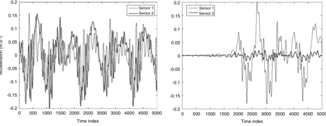
Fig. 1illustrates two hypothetical dynamic tests. Both tests in-troduced two sensors, each measuring a total of 5000 acceleration values. There are several ways to transform classical data into sym-bolic data. Let us consider, for instance, a signalXcontaining 5000 acceleration values measured by one singlesensor. This signal can be represented by

•

ann-class histogram:X

= {

1

(

0

.

0025

),

2

(

0

.

0721

),

3

(

0

.

8546

),

4

(

0

.

0626

), . . . ,

n(0

.

0082

)

}

;

•

a min/max interval:X

= [−

0

.

025

;

0

.

025

]

;

•

an interquartile interval:X

= [−

0

.

012

;

0

.

015

]

.

In this paper, two types of symbolic data are used in the SDA process: a 20-class histogram and interquartile intervals. Such statistical descriptions form a sort of filtering process since they reduce the amount of data to a smaller set. In turn, we can expect that nonlinear features, if existing, are not eliminated from this process. In order to obtain the first type of data (histogram valued), it is necessary to perform a projection of each measured value to the Y-axis of coordinates. Fig. 2 shows how to construct a histogram for eachsensorfrom each dynamictest. The divisions of a histogram are denominated classes. It must be noted that the same representation can be applied to modal parameters, i.e. natural frequencies and mode shapes. In other words, both of these quantities can be represented by intervals or histograms as described for the signals. Another important remark is that the process of transforming classical data to symbolic data is carried out almost instantly, which does not prohibit or make difficult the use of this methodology for a large ensemble of dynamic tests.

3. Principles of symbolic clustering methods

Data clustering is a common technique for statistical data analysis, which is used in many fields, including machine learning, data mining, pattern recognition, image analysis and bioinformatics [7]. A clustering procedure can be defined as a way of classifying a number of objects into different groups. More precisely, it can be described as the partitioning of a data set into subsets (clusters), so that the data in each subset share some common properties. In other words, for an appropriate clustering, it is necessary to minimize the within-cluster variation in order to obtain the most homogeneous clusters possible and, as a natural consequence, to maximize the between-cluster variation in order to obtain the most dissimilar clusters. In order to define these clusters and determine the proximity (or similarity) among the concepts, it is necessary to define suitable dissimilarity measures, which will be described in the next section.

3.1. Dissimilarity measures and within-cluster variations

The formation of clusters

(C

1

_{, . . . ,}

_Cr

₎

_{is governed by}

dissim-ilarity measures. These measures can supply numerical values in order to show the distance between two objects. In a common sense, the lower these values are the more similar the objects are, and thus they are gathered in the same cluster. Conversely, the objects allocated into different clusters are the ones which have greater distances between them. Cole [8] asserts that a small distance between two objects indicates ‘‘high’’ similarity. Thus, a distance measure can be used to quantify similarities as well as dissimilarities. Dissimilarity measures can take a variety of forms and some applications might require specific ones [9,10]. An im-portant step for any clustering method is to select a convenient dissimilarity measure. These measures will influence the shape of the clusters. For example, a given objectAmay be close to a given objectBaccording to one distance but distant according to another distance. In this work, for the interval-valued data, the Hausdorff distance is used, since it is faster to evaluate and it shows a better performance when compared to the other sym-bolic data distances presented in the literature. Let us consider two testsTi andTjwhich have their interquartile values represented

by

[

Ti,inf,Ti,sup

]

pand

[

Tj,inf,Tj,sup

]

pwithp

=

1

, . . . ,

nsensors,

respec-tively. The distance measure

φ(T

i

,

Tj

)

can be calculated as shown in

Eq.(1):

φ(T

i

,

Tj

)

=

nsensors

X

p=1

(

Max

[|

Ti,inf

−

Tj,inf

|

p

,

|

Ti,sup

−

Tj,sup

|

p

]

)

2

!

1/2

(1)

wherensensorsrepresents the number of sensors considered.

As previously mentioned, in order to get homogeneous clusters, it is necessary to minimize their within-cluster variationsI. The within-cluster variation of a clusterCkcontaining tests denoted by

Tican be calculated as

I(Ck

)

=

1

nnk

nk

X

i=1

nk

X

j>i=1

φ

2

(T

i

,

Tj

)

(2)

wherenis the total number of tests,nkis the number of tests within

clusterCk_and

_φ(T

i

,

Tj

)

are the elements of the dissimilarity matrix

and can be calculated according to Eq.(1), for instance.

For a given partitionPr

=

(C

1

, . . . ,

Cr

)

, the total within-cluster

variation W can be evaluated as the sum of all within-cluster variations [5]:

W(Pr

)

=

1

r r

X

k=1

I(Ck

₎

₍₃₎

whereris the number of clusters considered in the analysis. Similarly, the between-cluster variation can be defined by

B(Pr

)

=

W

(G)

−

W(Pr

)

(4)

whereGrepresents the global set of tests.

3.2. Clustering methods

The clustering simulations were carried out by using the soft-ware SODAS (Symbolic Official Data Analysis System), developed under the project ASSO (Analysis System of Symbolic Official Data). There are several clustering methods present in the literature. In this paper, three methods will be analyzed:

•

Hierarchy-divisive clustering, which is based on successive top-down divisions;

•

Hierarchy-agglomerative clustering, based on a bottom-up agglomeration process;

(4)

0.2

0.15

0.1

0.05

0

-0.05

-0.1

-0.15

-0.2

Time index Time index

Sensor 1 Sensor 2

0.2

0.15

0.1

0.05

0

-0.05

-0.1

-0.15

-0.2

0 500 1000 1500 2000 2500 3000 3500 4000 4500 5000 0 500 1000 1500 2000 2500 3000 3500 4000 4500 5000

Fig. 1. Example of two hypothetical dynamic tests.

0.025

0.02

0.015

0.01

0.005

0

-0.005

-0.01

-0.015

-0.02

-0.025

0 500 1000 1500 2000 2500 3000 3500 4000 4500 5000

Time index

1200

1000

800

600

400

200

0

Number of occurrences

-0.025 -0.02 -0.015 -0.01 -0.005 0 0.005 0.01 0.015 0.02 0.025 Classes

Fig. 2. Transforming classical data to symbolic data. 3.2.1. Hierarchy-divisive clustering

Divisive clustering is a top-down clustering process that starts with the entire data set as one cluster C and then proceeds downward through as many levels as necessary to produce the hierarchyY

=

(C

1

_,

_C2

_{, . . . ,}

_Cr

₎

_{. Theoretically, it is possible to}

have a number of clustersrmax where each cluster consists of a single test. In practice, however, the clustering process stops at an earlier stage. Typically, a maximum value forris specified, so that

r

<

rmax. Let us assume a single clusterCcontaining the entire set of tests denoted by

(T

1,T2, . . . ,Tn

)

and let us proceed by dividing

this cluster into two clusters (C1_and_C2_{). This procedure is carried}

out by determining which tests satisfy or not some logical criterion

q(.)(True or False). For instance, a criterion can be:q1—Is Sensor 4

≤

0

.

05 ms−2_{? If ‘‘True’’ (for the tests which satisfy the criterion),}

then they fall into the clusterC1_{; if ‘‘False’’, then those tests fall}

intoC2_{. In this example, ‘‘Sensor 4’’ and the value ‘‘0}

_.

_{05 m s}−2_’’

represent the variable and the cut-valuec which minimize the total within-cluster variationW of clustersC1 _and _C2_{. In other}

words, ‘‘Sensor 4’’ represents theexplicativevariable. Similarly, the explicative value and the cut-value can be expressed by means of the natural frequencies and the mode shapes, as well.

Fig. 3 shows a simplified scheme for the first partitioning procedure. The clustering process consists of two iterative procedures based on the number of sensors (nsensors) and on the number of cut-values corresponding to each sensor (ni

cv

,

i

=

1

, . . . ,

nsensors). Further details can be found in [5]. For each set (sensor, cut-value), both within-cluster and between-cluster

Fig. 3. Hierarchy-divisive algorithm.

variations are evaluated. This procedure is continued until the absolute minimal value for the sumWof within-cluster variations is obtained. Finally, the partitioning process will go on by taking into account the clusters corresponding to the minimalW value. The clustering process continues by partitioning the clusters C1

andC2_.

3.2.2. Hierarchy-agglomerative clustering

(5)

H(1,2)

H(2,3)

Distance between clusters

T1 T7 T8 T2 T10 T11 T3 T5 T4 T6 T9

Tests

1

2 ₃

Fig. 4. Example of a hierarchy-agglomerative clustering.

the hierarchy-divisive clustering is applied in reverse. Instead of starting with the complete set of tests and partitioning the cluster

Cinto two sub-clusters at each stage (C1_and_C2_{), the process starts}

withrclusters containing one single test and proceeds by merging two sub-clusters (C1_and_C2_{, say) into one new cluster}_C_{. The}

sub-clusters are merged according to similar criteria for minimizing the within-cluster variation and, consequently, for maximizing the between-cluster variation. More details can be found in [6]. This clustering method provides a measure of proximity between clusters when using the ‘‘difference in height’’ between them.Fig. 4

illustrates a hierarchy-agglomerative clustering procedure. In this example, clusters 1, 2 and 3 are highlighted. The heightsH(1

,

2

)

and H(2

,

3

)

represent the distances among them. As H(1

,

2

)

is greater thanH(2

,

3

)

, clusters 2 and 3 are closer than clusters 1 and 2.

3.2.3. Dynamic clouds

This clustering method is based on a generalization of the classical dynamical clusters method [6]. This method consists in minimizing a general optimized criterion that measures the adequacy between the partition and the representation of the clusters, denotedprototype. A prototype is a symbolic description model representing a cluster or, in other words, the ‘‘average’’ concept of a cluster. It is used as a reference to calculate the distances between the concepts and to define each cluster.

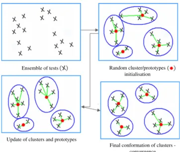
The algorithm initiates with a set ofkrandom prototypes and iteratively applies an allocation phase to place each concept in the cluster where the proximity between concept and prototype is minimal. In this process, a representation phase is performed where the prototypes are updated according to the allocation phase results. This is realized by computing and storing the total sum of the distances between concepts and the prototype in one cluster. The new cluster prototype is the one minimizing this sum. This two-phase procedure is repeated until convergence, that is, when the adequacy criterion reaches a stationary value (or at least when reaching a maximum number of iterations). In general, the dynamic cluster algorithm converges in a few iterations. In order to improve the quality of the clustering, the algorithm is executed with different initial partitions, and the best configuration is chosen among all the results.Fig. 5shows a simplified scheme of this clustering method.

4. Determination of the optimal number of clusters

Many different stopping rules have been published in the scientific literature. The most detailed and complete comparative

Ensemble of tests

Update of clusters and prototypes

Random cluster/prototypes initialisation

Final conformation of clusters -convergence

Fig. 5. Scheme representing the dynamic clouds algorithm.

study has been carried out by Milligan and Cooper [11]. They performed a Monte Carlo evaluation of 30 indices for the determination of the optimal number of clusters and they investigated the extent to which these indices were able to detect the correct number of clusters in a series of simulated data sets containing a known structure. In this section, the three best indices are presented: theCHindex, theC∗_{index and the}_Γ _{index [}₆_].

The general methodology for the evaluation of these three indices is based on calculating each one of them for a partition

Pm

=

(C

1

, . . . ,

Cm

)

containing a different number of clusters. The

number of clustersmis arbitrarily chosen and is greater thanr(the number of clusters previously considered in the analysis). Since

m

=

1 represents the partitionP1which only contains the initial cluster, the indices are not considered in this case.

TheCHindex is given by

CH(Pj

)

=

B(Pj

)

W

(P

j

)

×

(n

−

j)

(j

−

1

)

,

j

=

2

, . . . ,

m (5)

whereB(Pj

)

is the between-cluster variation,W

(P

j

)

is the total

within-cluster variation,nis the total number of tests andjis the number of clusters in the partitionPj. WhenCHhas itsmaximal absolute value, then the optimal partition (i.e. the optimal number of clusters) is obtained.

TheC∗_{index can be calculated as}

C∗

(P

j

)

=

1

n j

X

k=1

nk

(S

k

₋

_Sk min

)

(S

k

max

−

Smink

)

,

j

=

2

, . . . ,

m

;

C∗

∈ [

0

,

1

]

(6)

wherenis the total number of tests,nkis the number of tests of a

clusterCk_,_Sk_{represents the sum of distances among the}_k_tests

within a clusterCk_,_Sk

min is the sum of thek smallest distances

among all tests,Smaxk is the sum of theklargest distances among all

tests. The optimal partition is given whenC∗_{reaches its absolute} value.

TheΓindex is given by:

Γ

(P

j

)

=

Γ+

(P

j

)

−

Γ−

(P

j

)

Γ+

(P

j

)

+

Γ−

(P

j

)

,

j

=

2

, . . . ,

m

;

Γ

≤

1 (7)

whereΓ+

(P

j

)

represents the number of within-cluster distances

smaller than the between-cluster distances and Γ−

(P

j

)

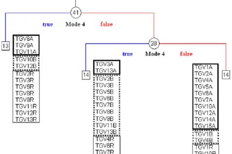
is the

(6)

Fig. 6. Classification of tests. Table 4

Definition of a new test and the prototypes described by sensors.

Test Sensor 1(m s−2₎ _{. . .} _Sensor_p₍_{m s}−2₎

T6 [0.03, 0.05] . . . [0.41, 0.62]

P∗

1 [0.06, 0.09] . . . [0.45, 0.87]

P∗

2 [0.04, 0.10] . . . [0.63, 0.89]

Table 5

Definition of a new test and the prototypes described by frequencies.

Test Frequency 1 (Hz) . . . Frequencynf(Hz)

T6 [5.77, 5.79] . . . [12.44, 12.63]

P∗

1 [4.89, 5.08] . . . [11.55, 12.78]

P∗

2 [5.84, 6.10] . . . [12.61, 13.09]

5. Classifying new tests

In this section, an original approach for classifying new tests is proposed. The main idea is to classify new dynamic tests according to the clusters defined by the methods previously described.

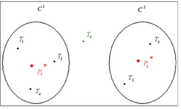
Let us consider a partition P2

=

(C

1

,

C2

)

containing two clusters, whereC1

₌

_(T1,

_T2,_T4)_and_C2

₌

_(T3,

_T5)_{. Let us also}

consider a new testT6and the prototypesP∗

1andP2∗representing

the clustersC1_and_C2_{, respectively (}_{Fig. 6}_).

The classification of the new test T6 will be performed by evaluating the distances between this test and the prototypesP∗

1

andP∗

2 of each cluster.Table 4can be assembled by considering

that each test is described by p sensors, where each sensor is represented by an interquartile interval. Similarly, Table 5

shows each test described bynf frequencies also represented by

interquartile intervals. The distance between the testT6and the prototypeP∗

1, denoted

φ(T6,

P1∗

)

, is evaluated by using Eq. (1).

Similarly, for the prototypeP∗

2, the distance is defined by

φ(T6,

P2∗

)

.

Finally, in order to make a conclusion about the relationship of the new test to clusterC1_{or to cluster}_C2_{, the following decision}

rules are employed:







φ(T6,

P₁∗

) < φ(T6,

P₂∗

)

⇒

T6

∈

C1

φ(T6,

P∗

1

) > φ(T6,

P2∗

)

⇒

T6

∈

C 2

φ(T

6,P∗

1

)

∼

=

φ(T

6,P2∗

)

⇒

T6

6∈

(C

1

∪

C2

).

For the last decision rule, a 5% error between the distances

φ(T

6,P∗

1

)

and

φ(T

6,P2∗

)

is applied.

6. Experimental results

6.1. Presentation of the case study

The studied bridge is an embedded steel bridge located on the South-East high-speed track in France at the kilometric point 075

+

317; it crosses the secondary road 939 between the towns of Sens and Soucy in Yonne county. A dynamic monitoring of this

railway bridge was performed to characterize and to quantify the effect of a strengthening procedure (Fig. 7). This strengthening pro-cedure consists in tightening special bearings in order to shift the first natural frequency (around 5 Hz) from the excitation frequency due to train crossings (around 4–5 Hz). The risk of resonance is thus increased, especially when ballast recharging occurs.

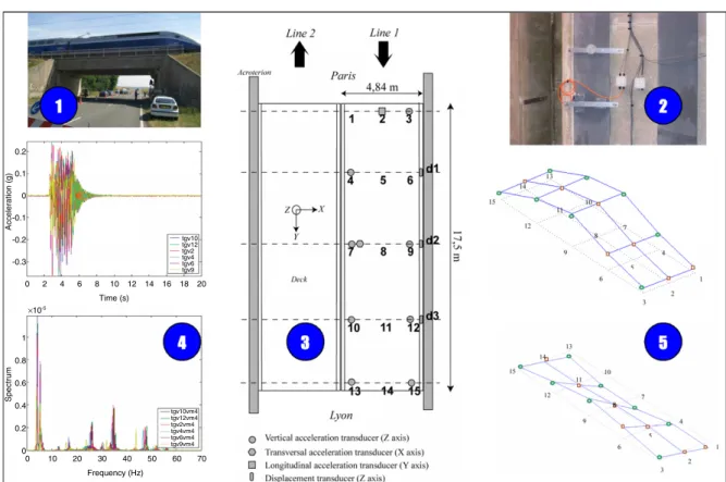
To be effective and relevant, dynamic testing must be precise about the selection of the test conditions (in particular of the source of excitation①), the choice of the data to acquire on a given frequency band②_{, the definition of the number and the localization} of the sensors③, the acquisition and the data processing④and the determination of the modal properties⑤_._{Fig. 8}_{illustrates these five} essential levels on the railway bridge PK 075

+

317.

The instrumentation comprises three vertical displacement sensors, eight vertical accelerometers and two horizontal ac-celerometers (longitudinal and transversal) under the bridge deck, two temperature gauges, and two Q sensors, which measure the axle loads at the entrance and at the clearance of the bridge. The sampling frequency was fixed at 4096 Hz. The signal analysis due to train crossings highlights a good repeatability [3]. In the follow-ing sections, only the acceleration measurements will be used for classification.

Three sets of dynamic tests were performed: before strength-ening (15 tests represented by the letter A), during (13 tests repre-sented by the letter R) and after (13 tests reprerepre-sented by the letter B). The idea is to make use of the symbolic data analysis in associa-tion with the clustering methods outlined in this paper in order to discriminate these three different stages. In other words, the goal is to break down the whole set of 41 tests into specific groups (before, during and after). In order to perform this task, the experimental data (signals), the natural frequencies and the mode shapes of the structure are used.

Modal parameters are extracted from the response measure-ments by the vectorial random decrement method [12]. This method requires fixing the model size (i.e. the number of modes present in the response). This disadvantage can be turned into an advantage by noting that automatically varying the model size can lead to getting an evaluation of the stability of the modal pa-rameters and therefore to assessing the good quality of the modal identification by generating histograms of the estimates. Fig. 9

gives a comparison between the first four modes before and af-ter strengthening. It comes that both modes 2 and 3 are the most sensitive to structural modification.

6.2. Classical frequency analysis

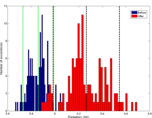
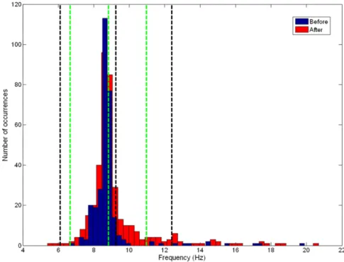
Before detailing the results obtained by using SDA methods, it is important to present a simple study consisting in analyzing the identified natural frequencies. Figs. 10–13show the histograms obtained for the first four natural frequencies, comparing the ‘‘before’’ and ‘‘after’’ states of the bridge. The dashed vertical lines represent the mean values and the limits of a 95% confidence interval of the identified frequencies.

Despite the fact that the difference between these two states is reasonably clear for the first frequency, this cannot be stated for the others. By simply analyzing the histograms, it is really difficult to distinguish these two states, since the values are superposed. It is therefore essential to use subsequent analyses in order to get a better discrimination.

6.3. Symbolic data analysis based on raw data (accelerations)

(7)

Fig. 7. Strengthening system and procedure.

Frequency (Hz) 0.2

0.1

0

-0.1

-0.2

-0.3

Acceleration (g)

0 2 4 6 8 10 12 14 16 18 20 Time (s)

1

0.8

0.6

0.4

0.2

0

Spectrum

0 10 20 30 40 50 60 70

Fig. 8. Schematic view of the instrumentation and data acquisition process. tests belonging to the ‘‘during’’ state which were classified into

wrong clusters. For example, the first cluster contains almost all the tests corresponding to the ‘‘before’’ state, but it contains two tests ‘‘TGV10R’’ and ‘‘TGV11R’’ which should correspond to the second cluster. It is essential to note that the tests corresponding to the ‘‘before’’ and ‘‘after’’ are identified into two distinct groups, except for the cluster ‘‘during’’, which presents erratic results. This observation shows that the strengthening effect is sensitive enough to be detected with this technique. Additionally, it is also possible to observe the two most explicative variables for this classification are Sensor 10 for the first level and Sensor 7 for the second division. For this method, 80% (12

/

15) of the ‘‘before’’ state were correctly classified as well as 70% (9

/

13) of the tests corresponding to the ‘‘during’’ state and 85% (11

/

13) for the ‘‘after’’ state. Finally,Table 6shows the ‘‘quality’’ indices evaluated for the clustering results obtained by this method. Despite bothCHand

Γindices giving correct results for an optimal partition with three clusters, theC∗_{index indicates an optimal number of four clusters.}

This could be explained by the fact that the noise inherent to the

Table 6

‘‘Quality’’ indices applied to the signals using the hierarchy-divisive method.

Clusters CH C∗ _Γ

5 18.35918 0.20701 0.64997

4 21.48122 0.16343 0.68355

3 29.99287 0.17755 0.71845

2 23.55649 0.18895 0.66721

1 – – –

data may strongly affect the results, especially for this case when raw measurements are used in this sort of analysis.

(8)

1

0

1

0

-1

1

0

-1

1

0

-1

0 17.5 35 52.5

Fig. 9. Comparison between interpolated mode shapes (before and after strengthening).

Fig. 10. Comparison between ‘‘before’’ and ‘‘after’’ states for the 1st frequency. Table 7

‘‘Quality’’ indices applied to the signals using the dynamic clouds method.

5 15.63371 0.15573 0.61479

4 19.80251 0.13385 0.57993

3 32.17181 0.14527 0.65877

2 24.62069 0.18503 0.64316

1 – – –

bothCHandΓ indices give correct results for an optimal partition with three clusters, but theC∗_{index indicates an optimal number}

of four clusters.

Finally,Fig. 16shows the results for the hierarchy-agglomerative method using the signals transformed into interquartile intervals. The clusters are indicated by 1, 2 and 3 in order to highlight each group of tests. For this method, a larger quantity of tests was not correctly classified. This could be explained by the criteria used for

gathering the closest tests and assembling the clusters. In other words, this clustering method may not be sensitive enough to iden-tify and discriminate structural modifications. Consequently, 60% (9

/

13) for the ‘‘after’’ state. Finally,Table 8shows the ‘‘quality’’ in-dices evaluated for this method. For this case, only theCHindex indicates an optimal partition with three clusters. BothC∗_and_Γ

indices indicate an optimal number of four clusters. These results are directly influenced by the fact that percentages of correct clas-sifications were lower compared to the previous methods.

6.4. Symbolic data analysis based on modal parameters

(9)

Fig. 11. Comparison between ‘‘before’’ and ‘‘after’’ states for the 2nd frequency.

Fig. 12. Comparison between ‘‘before’’ and ‘‘after’’ states for the 3rd frequency. Table 8

‘‘Quality’’ indices applied to the signals using the hierarchy-agglomerative method.

5 17.44663 0.22457 0.69961

4 22.10789 0.19645 0.77210

3 35.58992 0.15889 0.71384

2 28.83197 0.15320 0.72025

1 – – –

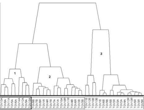
the hierarchy-divisive method applied to the natural frequencies transformed into interquartile intervals. It is possible to notice the existence of three clusters containing almost the sets of tests corresponding to each structural state. As for the raw data analysis, there are some tests belonging to the ‘‘during’’ state that are

classified in the cluster ‘‘after’’. The two most explicative variables for this clustering process are highlighted: Frequency #4 for the first division and Frequency #3 for the second one. It is interesting to note that Frequency #1 is not the explicative variable although the frequency shift is a priori the most sensitive. The proportions of correct classification were 87% (13

/

15) for the ‘‘before’’ state, 85% (11

/

13) for the ‘‘during’’ state and 92% (12

/

13) for the ‘‘after’’ state. Additionally,Table 10presents the results obtained for the ‘‘quality’’ indices using the dynamic clouds method. In this case, the three indicesCH,C∗_and_Γ_{point towards the expected results,}

i.e. optimal clustering with three clusters.

(10)

Fig. 13. Comparison between ‘‘before’’ and ‘‘after’’ states for the 4th frequency.

Fig. 14. Hierarchy-divisive method applied to the signals (raw data). Table 9

First natural frequencies identified at each strengthening stage. Frequencies Before

modification

During modification

After modification

i f(Hz) f(Hz) f(Hz)

1 5.84 6.27 6.44

2 8.61 8.74 8.78

3 13.09 13.20 13.31

4 16.95 17.21 17.34

Table 10

‘‘Quality’’ indices applied to the natural frequencies using the hierarchy-divisive method.

5 26.48091 0.12953 0.66331

4 27.87751 0.11588 0.79024

3 33.96248 0.10746 0.82946

2 22.13904 0.12377 0.72175

1 – – –

Table 11

‘‘Quality’’ indices applied to the natural frequencies using the dynamic clouds method.

5 29.69278 0.19945 0.61898

4 21.49616 0.06928 0.62116

3 39.21571 0.06404 0.76369

2 24.31680 0.07795 0.69231

1 – – –

Table 12

‘‘Quality’’ indices applied to the natural frequencies using the hierarchy-agglomerative method.

5 24.4417 0.42466 0.58997

4 27.1738 0.33948 0.63548

3 38.3003 0.14192 0.79225

2 32.0112 0.01797 0.63541

1 – – –

a couple of tests are also badly classified. In fact, 93% (14

/

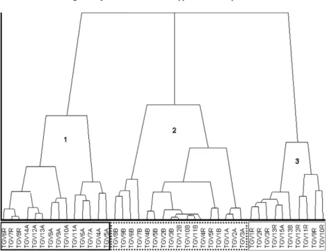
13) for the ‘‘after’’ state.Table 11presents the results obtained for the ‘‘quality’’ indices using the dynamic clouds method. Again, all three indices indicate three clusters as the optimal partition.

Finally,Fig. 19shows the results obtained for the hierarchy-agglomerative method using the natural frequencies transformed into interquartile intervals. The clusters are indicated by 1, 2 and 3 in order to highlight each group of tests. Moreover, 73% (11

/

13) for the ‘‘after’’ state. In addition,Table 12shows the ‘‘quality’’ indices evaluated for this method. For this case, bothCHandΓ indices indicate an optimal partition with three clusters. However, theC∗

index indicates an optimal number of two clusters. These results are directly influenced by the fact that percentages of correct classifications were lower compared to the previous methods.

(11)

Fig. 15. Dynamic clouds method applied to the signals (raw data).

Fig. 16. Hierarchy-agglomerative method applied to the signals (raw data).

where mode shapes were converted to interquartile intervals. As for the previous classifications, a couple of mode shapes were incorrectly classified in their respective clusters. The proportions of correct classification were 67% (10

/

13) for the ‘‘after’’ state. For this case, a larger occurrence of misclassifications is observed. Mode #4 is in this case the explicative variable.

Furthermore, the dynamic clouds method is applied to the same modal data (now converted to a 20-class histogram) and similar results are obtained (Fig. 21). For this method, 60% (9

/

13) for the ‘‘after’’ state.

Finally,Fig. 22presents the results obtained when a hierarchy-agglomerative clustering method is applied to the mode shapes transformed into interquartile intervals. Similarly to the analysis performed with the signals, it is possible to observe a large number of mode shapes that are badly clustered. This can be due to the

(12)

Fig. 18. Dynamic clouds method applied to the frequencies.

Fig. 19. Hierarchy-agglomerative method applied to the frequencies. a suitable discrimination criterion among the mode shapes. The

proportions of correct classification were 47% (7

/

13) for the ‘‘after’’ state.

Taking all of these results into consideration, it is possible to conclude that the SDA applied to the natural frequencies presented better classifications when compared to those obtained by using signals and mode shapes. In fact, the first two clustering methods i.e. hierarchy-divisive and dynamic clouds, produced more homogeneous groups and with better ratios of correct classification. Nevertheless, the results obtained by using the SDA applied to the signals were quite convincing. It should also be noted that the presence of noise might have circumvented the achievement of better classification results.

6.5. Classification of new tests

In this section, the proposed approach for the classification of new tests is introduced using alternatively raw data (signals) and natural frequencies. In this case, it is considered that:

•

five tests were randomly chosen among the 15 tests represent-ing the ‘‘before’’ state of the bridge: TGV1A, TGV5A, TGV6A, TGV9A and TGV14A;

•

five tests were randomly chosen among the 13 tests repre-senting the ‘‘after’’ state of the bridge: TGV1B, TGV4B, TGV9B, TGV11B and TGV12B;

•

five different tests (considering both ‘‘before’’ and ‘‘after’’ states of the bridge) were randomly chosen and assigned as ‘‘new’’ tests: TGV8A, TGV10A, TGV5B, TGV7B and TGV13B.

The methodology consists in applying the three clustering methods described in Section3to the first two sets of five tests in order to form two clusters, where each one should represent one state of the bridge. In other words, clusterC1_{should only contain}

the set of five ‘‘before’’ tests and clusterC2_{should only contain the}

(13)

Fig. 20. Hierarchy-divisive method applied to the mode shapes.

Fig. 21. Dynamic clouds method applied to the mode shapes.

(14)

Table 13

Classification of new tests/signals.

Tests φ(Ti,P1) φ(Ti,P2) Detected cluster True cluster

TGV8A 0.050 0.063 C1 _C1

TGV5B 0.098 0.071 C2 _C2

TGV10A 0.088 0.079 C2 _C1

TGV7B 0.064 0.038 C2 _C2

TGV13B 0.047 0.025 C2 _C2

Table 14

Classification of new tests/frequencies.

Tests φ(Ei,N1) φ(Ei,N2) Detected cluster True cluster

TGV8A 0.60 0.87 C1 _C1

TGV5B 0.70 0.66 C2 _C2

TGV10A 0.73 0.79 C1 _C1

TGV7B 0.87 0.48 C2 _C2

TGV13B 2.32 1.25 C2 _C2

check whether the classification will be robust or not. In view of the fact that all clustering methods obtained the same prototypes, the classification results are the same. InTable 13, the values inbold

represent the smallest distance between the new tests and the cluster’s prototypes. This will define the classification of each test. For this classification, all tests were correctly classified, except the test TGV10A, which should be classified within clusterC1_(before

modification) but was classified within clusterC2_{. This result may}

be due to noise present in the signals.

The same methodology is considered when using the nat-ural frequencies. Table 14 gives the values (in bold) repre-senting the smallest distance between the new tests and the cluster’s prototypes. For this classification, all tests were correctly classified.

7. Conclusions and remarks

In this paper a novel technique based on symbolic data analysis was introduced in order to classify different structural behaviors. For this purpose, raw information (acceleration measurements) as well as processed information (modal data) were used for feature extraction. Some SDA techniques were applied for data classification: hierarchy-divisive methods, dynamic clustering and pyramid schemes.

An experimental application containing three structural states of a railway bridge located in France was studied. The objective was to use the clustering methods applied to the data in order to discriminate the structure’s different conditions. The results obtained showed that the SDA methods are efficient in classifying and discriminating structural modifications either considering the vibration data or the modal parameters.

In fact, both the hierarchy-divisive and the dynamic clouds methods produced better results compared to those obtained by using the hierarchy-agglomerative method. This can be due to the intrinsic characteristics of each method (i.e. the choice of a discrimination criterion as well as the pertinence of a dissimilarity measure used). Indeed, more robust results are given by all

clustering methods when applied to modal data than when applied to measurement data. The presence of relevant noise levels into the latter one can clearly justify this observation.

Moreover, the results obtained by classical analyses showed to be not sensitive enough to point out the presence of structural modifications. By performing a simple examination of the frequency histograms it was impossible to distinguish all the different structural states of the bridge (except for the first frequency). It was therefore considered essential to use subsequent analyses in order to get better discrimination.

These preliminary results highlighted that it is indispensable to compare different clustering methods, since it is possible to have either good or bad clusters by using the same input data. For this purpose, three ‘‘quality’’ indices were introduced:CH,C∗_and_Γ_.

The main idea was to find the optimal number of clusters that should be obtained after a clustering process. Firstly applied to signals, one of those indices presented a wrong optimal partition. Again, this could be due to the noise present in the data. However, when applied to the natural frequencies, all the indices gave results in agreement with tests conditions.

Finally, an original approach for classifying new dynamic tests according to the clusters previously defined was presented. Once again, the results obtained with the natural frequencies were reasonably better compared to those using the signals. The different results highlighted the large capability of the SDA methods to provide on the one hand clusters of different structural conditions, and on the other hand to test new data versus these clusters. The presented SDA techniques are therefore sensitive enough to be used as a learning procedure and as a test procedure for classifying and detecting structural modifications.

References

[1] Doebling SW, Farrar CR, Prime MB, Shevitz DW. Damage identification and health monitoring on structural and mechanical systems form changes in their vibration characteristics: A literature review. Los Alamos National Laboratory, Report LA-13070-MS; 1996.

[2] Rytter A. Vibration based inspection of civil engineering structures. Ph.D. dissertation. Denmark: Department of Building Technology and Structural Engineering, Aalborg University; 1993.

[3] Cremona C. Dynamic monitoring applied to the detection of structural modifications. A high speed railway bridge study. Prog Struct Mat Eng 2004; 3:147–61.

[4] Hastie T, Tibshirani R, Friedman J. The elements of statistical learning: Data mining, inference, and prediction. second ed. Springer series in statistics, 2009. [5] Billard L, Diday E. Symbolic data analysis. Wiley; 2006.

[6] Diday E, Noirhomme-Fraiture M. Symbolic data analysis and the SODAS software. Wiley; 2008.

[7] Bock HH, Diday E. Analysis of symbolic data. Springer; 2001.

[8] Cole RM. Clustering with genetic algorithms. M.Sc. thesis. Australia: Depart-ment of Computer Science, University of Western Australia; 1998.

[9] Malerba D, Esposito F, Gioviale V, Tamma V. Comparing dissimilarity measures for symbolic data analysis. ETK-NTTS 2001, Hersonissos, Crete. Vol. 1. 2001. p. 473–81.

[10] Malerba D, Esposito F, Monopoli M. Comparing dissimilarity measures for probabilistic symbolic objects. Data mining III, series management information systems, Vol. 6. Southampton, UK: WIT Press; 2002. p. 31–40. [11] Milligan GW, Cooper MC. An examination of procedures for determining the

number of clusters in a data set. Psychometrika 1985;50:159–79.