Biodiversity informatics - entomological data processing, analysis and visualization

(1)

2019

UNIVERSIDADE DE LISBOA

FACULDADE DE CIÊNCIAS

DEPARTAMENTO DE BIOLOGIA ANIMAL

Biodiversity informatics – Entomological data processing,

analysis and visualization

Leonor Fernanda Venceslau Azeredo Pontes

Mestrado em Bioinformática e Biologia Computacional

Dissertação orientada por:

Doutora Alexandra Marçal Correia

(2)

i

Acknowledgements

First of all, a big thank you to my advisors, Dr. Luis Filipe Lopes and Dr. Alexandra Marçal Correia. They gave me the opportunity of working in a fascinating project and they were always available whenever I had doubts or needed help.

I would also like to thank all the colleagues and friends at the Zoology department of the Museu

Nacional de História Natural e da Ciência, including, but not limited to: Isabel Queirós Neves,

Leonor Brites Soares, Diogo Parrinha, Dr. Paula Souto, Dr. Alexandra Cartaxana, Dr. Cristiane Bastos-Silveira and Dr. Judite Alves. In different ways, they all contributed to help me with this work, either during the first months or later when I was working with a research fellowship at the Museum while finishing this project.

To Professor Luis Mendes, for help with finding the Tabanidae specimens of the collections of the Instituto de Investigação Científica Tropical and their records; the digitization process would have been much harder without his help. To Dr. Hélcio Gil, for the valuable information about Tabanidae species, and for verifying taxonomic identifications of the specimens to add more information to the Tabanidae dataset.

To everyone at the Instituto de Higiene e Medicina Tropical who welcomed me and provided insight during the process of digitization of the Tabanidae collection of the IICT.

I would like to thank my family for all the love and support without which it wouldn’t have been possible to complete this work. To Diogo Simões, for being there for me everytime I needed, listening and helping with every problem along the way. To my mother, my father, my brother, my sister and my grandparents. They all believed in me unconditionally and helped me believe in myself.

And finally, to everyone not mentioned here, but who directly or indirectly helped me during this work, thank you!

(3)

ii

Abstract

This work is based on data records associated with the insect Collections from the Museu

Nacional de História Natural e da Ciência (MNHNC) and Instituto de Investigação Científica Tropical (IICT), Universidade de Lisboa. In 2014 a dataset with 30 535 records was published in

the Global Biodiversity Information Facility (GBIF). Since then data has been improved and new records acquired. Currently, the collection catalogue includes 39 139 validated records, corresponding to 79 885 specimens, with much more to be added from collections donated by private collectors or unprocessed samples. The data for these specimens was cleaned, formatted and geocoded and published on the GBIF.

During this work, different APIs were tested to allow automated geocoding of sampling locations. Google Maps achieved the best results, with 57.6% of results within 1000 m of the correct location. A citizen science project was developed and tested to accelerate the digitization process, including two workflows with different objectives. One was focused on the transcription of specimen label data, which resulted in the data for 130 specimens being successfully transcribed. The other was focused on the taxonomic identification of specimens from photographs, directed to specialists in the respective group’s taxonomy, which resulted in 61 new identifications and the verification of identifications for the remaining 69 specimens.

The MNHNC and IICT collections contain collections of horseflies (Order Diptera, Family Tabanidae) which are of particular importance due to its size and completeness of associated data. Horseflies are widely distributed worldwide and are important vectors in transmission of diseases to humans and cattle. The IICT collection includes a sub-collection which was compiled and studied by J. A. Travassos Santos Dias, a prominent specialist in this group. The specimens in these collections were photographed, all the associated data were transcribed, taxonomic identifications were verified and records were geocoded, resulting in a dataset of 1666 specimens. These specimens were collected between 1899 and 2018, mainly in Portugal, but also in São Tomé and Príncipe, Guinea-Bissau, Mozambique, Spain and other countries. To better understand the distribution of this group, distribution maps were made for the most well-represented species in the collections.

Keywords

(4)

iii

Resumo alargado

Este trabalho foca-se na digitalização, tratamento e análise de dados de colecções de história natural fazendo uso de ferramentas da informática da biodiversidade. Foram usados dados das colecções de insectos do Museu Nacional de História Natural e da Ciência (MNHNC) e do Instituto de Investigação Científica Tropical (IICT), Universidade de Lisboa. Em 2014, um

dataset com 30 535 registos da colecção de insectos do MNHNC foi publicado no Global Biodiversity Information Facility (GBIF). Desde então, novos registos foram digitalizados e

foram adicionados novos dados, tais como novas identificações taxonómicas, entre outros. Actualmente, o catálogo da colecção de insectos do MNHNC inclui 39 139 registos validados, que correspondem a cerca de 98% do total, referentes a 79 885 espécimes. Para que este dataset actualizado pudesse ser publicado, foram aplicadas ferramentas de limpeza de dados para detecção e correcção de erros, bem como a georreferenciação de registos, de forma a que os dados possam ser localizados num mapa a partir das coordenadas. Relativamente à limpeza e homogeneização de dados, todos os campos foram limpos e formatados de acordo com as normas do modelo de metadados DarwinCore. Este processo incluiu a verificação de identificações taxonómicas para detectar sinonímias e erros ortográficos, alteração do formato de datas e horas, e aplicação de um vocabulário controlado para os restantes campos.

Paralelamente a este processo, foram testadas ferramentas para acelerar a digitalização em duas fases diferentes: transcrição e georreferenciação de dados a partir de etiquetas de espécimes. Foram testadas cinco ferramentas de georreferenciação que disponibilizam Application

Programming Interfaces (APIs), que podem ser usadas para georreferenciar registos

automaticamente a partir de nomes de localidades: Google Maps, MapQuest, GeoNames,

OpenStreetMap e GEOLocate. Destes, a ferramenta Google Maps foi a que produziu melhores

resultados, com 57.6% dos resultados a uma distância de 1000 m ou menos do local correcto. Foi também desenvolvido e testado um projecto de ciência cidadã na plataforma Zooniverse, que contemplou duas vertentes: uma de transcrição de dados a partir de fotografias de espécimes com etiquetas, direccionada ao público geral, e uma de identificação taxonómica de espécimes a partir de fotografias, direcionada a especialistas na taxonomia do respectivo grupo. A primeira vertente resultou na transcrição com sucesso dos dados de todos os 130 espécimes disponibilizados. A segunda resultou na identificação dos 61 espécimes que não tinham identificação prévia, e na verificação das identificações dos restantes 69 espécimes. Conclui-se, portanto, que os projectos de ciência cidadã serão uma boa maneira de acelerar o projecto de digitalização, desde que sejam implementados métodos de verificação e correcção de erros adequados.

Por forma a focar todos os passos do processo de digitalização de uma forma mais completa, foram selecionadas as colecções de tabanídeos (Diptera: Tabanidae) do IICT e do MNHNC. Este grupo é de especial interesse por incluir importantes vectores de transmissão de doenças a humanos e gado, e por ter uma distribuição ampla em todo o Mundo. A colecção de tabanídeos do IICT é particularmente importante por ter sido, na sua maioria, compilada e estudada por J. A. Travassos Santos Dias, um especialista neste grupo que publicou extensos trabalhos com base nos espécimes da colecção. Ambas as colecções incluem espécimes tipo de espécies descritas por Travassos Santos Dias e outros autores. Apesar da sua importância, a informação associada aos espécimes das colecções do IICT/MNHNC ainda não estava digitalizada. Neste trabalho, foram fotografados todos os espécimes e transcritos os seus dados, resultando num dataset com 1 666 exemplares. Foi feita a georreferenciação dos registos sempre que possível. Os espécimes da colecção foram recolhidos entre 1899 e 2018, maioritariamente em Portugal, mas também em São

(5)

iv Tomé e Príncipe, Guiné-Bissau, Moçambique, Espanha e outros países. Para uma melhor visualização da distribuição geográfica dos espécimes, foram criados mapas de distribuição, recorrendo a R, para as espécies mais bem representadas nas colecções. A publicação deste dataset na plataforma GBIF será uma mais-valia para o estudo da distribuição deste grupo, devido à sua ampla cobertura geográfica e temporal, bem como ao facto da maioria dos espécimes (85.1%) estarem identificados até à espécie ou subespécie.

Palavras-chave

Colecções de história natural; digitalização de dados; limpeza de dados; georreferenciação; ciência cidadã

(6)

1

List of Figures

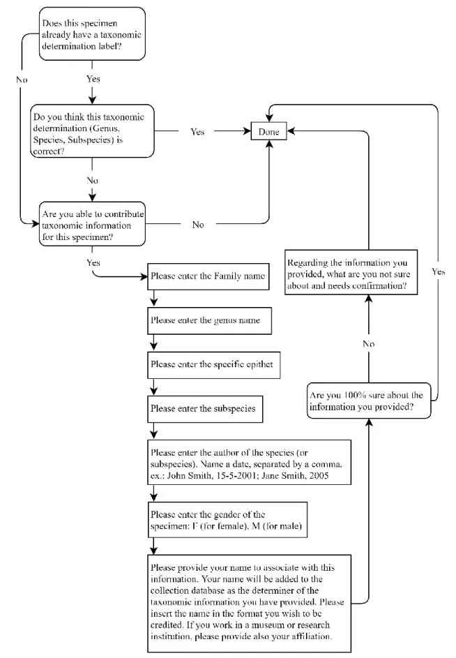
Figure 3.1 Steps employed in data cleaning and visualization for the MNHNC insect collection catalogue. ... 16 Figure 3.2 Histogram of specimens of the MNHNC insect collection by decade of collection. ... 18 Figure 3.3 Bar graph of specimens of the MNHNC insect collection by sampling country. The plot includes the countries where 100 or more specimens were sampled. ... 19 Figure 3.4 Percentage of specimens of the insect collection catalogue identified to each taxon rank, in the dataset published on GBIF in 2014 (A) and in the dataset published in 2019 (B). In (A), Class is omitted for clarity, accounting for 0.4% of specimens... 20 Figure 3.5 Bar graph of specimens of the MNHNC insect collection by Order. The plot includes the Orders represented by more than 100 specimens in the collection. ... 20 Figure 3.6 Bar graph of specimens of the MNHNC insect collection by Family. The plot includes the Families represented by more than 200 specimens in the collection. ... 21 Figure 4.1 Flowchart representing the tasks in the transcription workflow of the project developed on the Zooniverse platform. Rectangles represent tasks where the user is prompted for text input, squared rectangles represent multiple answer questions. ... 25 Figure 4.2 Flowchart representing the tasks in the taxonomic identification workflow of the project developed on the Zooniverse platform. Rectangles represent tasks where the user is prompted for text input, squared rectangles represent multiple answer questions. ... 26 Figure 4.3 Image of the first task that volunteers were asked to complete in the transcription workflow of the project developed on the Zooniverse platform. ... 27 Figure 4.4 Transcriptions made by volunteers per day, between December 2018 and April 2019. Each transcription corresponds to completing all the tasks by one volunteer. Each image is transcribed by more than one volunteer. ... 28 Figure 4.5 Contributions to the taxonomic workflow made by volunteers per day, between December 2018 and March 2019. Each contribution corresponds to either a transcription and confirmation of taxonomic identification labels in one specimen, or a new taxonomic identification of a specimen, done by a volunteer. Each image can be classified by more than one volunteer. ... 29 Figure 4.6 Answers by volunteers to the question “How easy or difficult did you find the task?” in the feedback survey for the Zooniverse project. The survey was filled out by 32 volunteers who contributed with a classification. ... 30 Figure 4.7 Answers by volunteers to the question “In your opinion, is this project suitable for the Zooniverse?” in the feedback survey for the Zooniverse project. The survey was filled out by 32 volunteers who contributed with a classification. ... 30 Figure 4.8 Answers by volunteers to the question “If we decide to launch this project publicly, do you think you will take part?” in the feedback survey for the Zooniverse project. The survey was filled out by 32 volunteers who contributed with a classification. ... 31

(8)

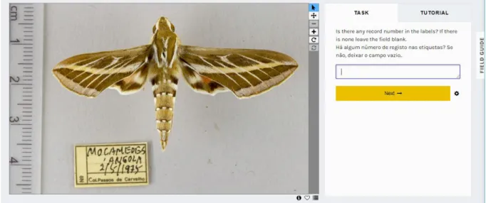
3 Figure 5.1 - Example of a photograph of a specimen of the Tabanid collection, with collection and classification labels... 35 Figure 5.2 Percentage of tabanid specimens in the IICT/MNHNC collections identified to each taxon rank. ... 36 Figure 5.3 Bar graph of tabanid specimens in the IICT/MNHNC collections by Genus, for Genera represented by 10 or more specimens in the collections. ... 37 Figure 5.4 Bar graph of tabanid specimens in the IICT/MNHNC collections by species. Species represented by 20 or more specimens in the collection are shown. ... 37 Figure 5.5 Bar graph of Tabanidae specimens in the IICT/MNHNC collections by sampling country. Countries represented by 10 or more specimens in the collections are shown. ... 43 Figure 5.6 Histogram of tabanid specimens in the IICT/MNHNC collections by sampling year aggregated per decade. ... 43 Figure 5.7 World map representing the countries where Tabanidae specimens of the IICT/MNHNC collections were collected. Circle size represents the number of specimens collected in each country. ... 44 Figure 5.8 Map of sampling locations of Tabanidae of the IICT/MNHNC collections in Portugal. Circle size represents the number of specimens sampled at each location. Inset shows the Azores islands. .. 45 Figure 5.9 Collection location for specimens of Tabanus monocallosus of the IICT/MNHNC collection collected in São Tomé and Príncipe, in the islands of (A) São Tomé and (B) Príncipe. Circle size corresponds to the uncertainty area for each sampling location, fill colour represents the number of specimens collected. ... 46 Figure 5.10 Countries where sampling of specimens of Tabanus eggeri has been registered on GBIF (blue) and where T. eggeri specimens of the IICT/MNHNC collections were sampled (yellow). Portugal, which has occurrences of T. eggeri registered on GBIF and is also represented in the MNHNC/IICT collections is shown in green. ... 47 Figure 5.11 Locations where specimens of Tabanus eggeri in the IICT/MNHNC collections were collected. Circle size represents the geocoding uncertainty of the sampling locality, for localities with uncertainty greater than 3000 m. Locations with geocoding uncertainty smaller than 3000 m are represented by lozenges. In both cases, fill color represents the number of specimens collected in each location (minimum = 1, maximum = 27). ... 48 Figure 5.12 Countries where sampling of specimens of Haematopota italica has been registered on GBIF (blue) and where H. italica specimens of the IICT/MNHNC collections were sampled (red). .. 49 Figure 5.13 Locations where specimens of Haematopota italica in the IICT/MNHNC collections were collected. Circle size represents the geocoding uncertainty of the sampling locality, for localities with uncertainty greater than 2500 m. Locations with geocoding uncertainty smaller than 2500 m are represented by lozenges with black trim. In both cases, fill color represents the number of specimens collected in each location (minimum = 1, maximum = 34). ... 50

(9)

4 Figure 5.14 Countries where Tabanus autumnalis specimens have been registered on GBIF (blue) and in the IICT/MNHNC collections (yellow). The only country where specimens of T. autumnalis of the IICT/MNHNC collections were sampled and where there are occurrences of this Species registered on GBIF is Spain, shown in green. ... 51 Figure 5.15 Locations where specimens of Tabanus autumnalis in the IICT/MNHNC collections were sampled. Circle size represents the geocoding uncertainty of the sampling locality, for localities with uncertainty greater than 2500 m. Locations with geocoding uncertainty smaller than 2500 m are represented by lozenges with black trim. In both cases, fill color represents the number of specimens collected in each location (minimum = 1, maximum = 3). ... 52 Figure 5.16 Sampling location for the specimen of Tabanus autumnalis in the IICT/MNHNC collections sampled in São Miguel island, Azores. ... 52 Figure 5.17 Countries where Tabanus sudeticus specimens have been registered on GBIF (blue) and in the IICT/MNHNC collections (yellow). The countries where specimens of T. sudeticus of the IICT/MNHNC collections were sampled and where there are occurrences of this Species registered on GBIF are Spain and France, shown in green. ... 53 Figure 5.18 Sampling locations of Tabanus sudeticus specimens from Portugal found in the IICT/MNHNC collections. Circle size represents the geocoding uncertainty of the sampling locality, for localities with uncertainty greater than 2500 m. Locations with geocoding uncertainty smaller than 2500 m are represented by lozenges with black trim. In both cases, fill color represents the number of specimens collected in each location (minimum = 1, maximum = 18). ... 54 Figure 5.19 Sampling locations of Tabanus sudeticus specimens in the IICT/MNHNC collections sampled in Portugal (32 specimens), Spain (10 specimens, all in the same location in Andalucia) and France (1 specimen). ... 55 Figure 5.20 Countries where sampling of specimens of Tabanus bromius have been registered on GBIF (blue) and where T. bromius specimens of the IICT/MNHNC collections were sampled (red). ... 56 Figure 5.21 Locations where specimens of Tabanus bromius in the IICT/MNHNC collections were collected, in the (A) North and (B) South of Portugal. Circle size represents the geocoding uncertainty of the sampling locality, for localities with uncertainty greater than 2500 m. Locations with geocoding uncertainty smaller than 2500 m are represented by lozenges with black trim. In both cases, fill color represents the number of specimens collected in each location (minimum = 1, maximum = 10). ... 57 Figure 5.22 Locations where specimens of Tabanus barbarus in the IICT/MNHNC collection were collected. Circle size represents the geocoding uncertainty of the sampling locality, for localities with uncertainty greater than 1000 m. Locations with geocoding uncertainty smaller than 1000 m are represented by lozenges with black outlines. In both cases, fill color represents the number of specimens collected in each location (minimum = 1, maximum = 7). ... 58 Figure 5.23 Countries where occurrences of Ancala fasciata have been registered on GBIF (blue) and in the IICT/MNHNC collections (red). ... 59 Figure 5.24 Locations where specimens of Ancala fasciata in the IICT/MNHNC collections were sampled. Circle size represents the uncertainty of the sampling locality. Circle color represents the number of specimens sampled in each location (minimum = 1, maximum = 22). ... 59

(10)

5 Figure 5.25 Locations where specimens of Tabanus mesquitelai in the IICT/MNHNC collections were sampled. Circle size represents the uncertainty of the sampling locality. Circle color represents the number of specimens sampled in each location (minimum = 4, maximum = 14). ... 60

(11)

6

List of Tables

Table 2.1 Results of geocoding 100 insect records with the 5 APIs tested. Coordinates and uncertainty radius for the reference location of each record were obtained by geocoding using the GEOLocate Web Application, confirmed by Google Maps where necessary. Distance to the reference location for each result was calculated using the 'Vincenty' (ellipsoid) great circle distance function. ... 11 Table 2.2 Results of geocoding 100 insect records with complex location descriptions, with the 5 APIs tested. Coordinates and uncertainty radius for the reference location of each record were obtained by geocoding using the GEOLocate Web Application, confirmed by Google Maps where necessary. Distance to the reference location for each result was calculated using the 'Vincenty' (ellipsoid) great circle distance function. ... 12 Table 5.1 Type specimens of the IICT tabanid collection. The number of holotypes, allotypes and paratypes in the collection is accounted for each species. Scientific name refers to the species described by the author. For the cases where the species was later considered a synonym of another the updated name is given under Current name. ... 39 Table 5.2 Type specimens of the MNHNC tabanid collections. The number of holotypes, allotypes and paratypes in the collections is accounted for each species. Scientific name refers to the species described by the author. For the cases where the species was later considered a synonym of another the updated name is given under Current name. ... 42

(12)

7

1. Introduction

Natural history collections (NHC) are a powerful source of information for research with many possible applications. They are essential for systematic studies, since type specimens used to describe species are stored there and constitute an important reference. Moreover, many new species are identified from specimens in these collections [1]. Often, specimens stored in museums represent species that would be difficult or impossible to collect or study in the present time, due to population reduction or extinction, costs of revisiting field sites or restrictive export policies [2]. These collections can be used for training taxonomic specialists [3, 4] and the information contained in these records can be used for population distribution analysis and modelling, for molecular biology and morphology studies [5–7], as well as to define strategies to deal with ecosystem changes due to issues such as climate change, deforestation, overfishing, infectious diseases, and invasive species [8–10]. According to Drew (2011), conservation biology benefits from natural history institutions in three main ways: collection-based research projects and taxonomic expertise, collections data digitization and public engagement. Because NHC usually contain specimens collected over several decades or even centuries, they hold data that can be used for studies across long periods of time [3]. By combining data from several collections, especially if it is available online and in a standardized format, studies can be conducted within wide geographic and temporal ranges, allowing large scale analyses of changes in biodiversity and species distribution. In 2002, the Convention on Biological Diversity, ratified by 196 Countries, set a target to significantly reduce the worldwide rate of biodiversity loss by 2010, which was incorporated in the United Nations Millennium Development Goals. Not only this target was missed, but also some of the factors contributing to biodiversity loss have increased in this period. The five main factors identified by member countries were habitat loss, the unsustainable use and overexploitation of resources, climate change, invasive alien species, and pollution. Some of the main obstacles pointed out to achieving a reduction on biodiversity loss were the lack of scientific information and lack of awareness among the public and decision makers regarding this issue [11]. Making biodiversity data freely accessible, not only to the scientific community but also to Governments and the general public, will be an important step to raise awareness and generate the necessary detailed information to drive conservation measures to counter biodiversity loss [12]. This illustrates the importance of making biodiversity data publicly accessible, in particular that of NHC, as they represent a rich source of information. As technology advances, NHC specimens and record data will have even more applications [9]. In fact, there have been concerted global efforts to digitize these collections and to make that information public [9, 13]. Thousands of biodiversity datasets, related to NHC, observation data, and others, have been published on digital repositories, where they can be freely accessed and retrieved for analysis. For instance, the Global Biodiversity Information Facility (GBIF, www.gbif.org) currently includes over 45 000 datasets, including data from NHC, field observations, among others; the Integrated Digitized Biocollections portal (iDigBio, www.idigbio.org/) contains over 1 600 NHC datasets. Despite this effort and the importance and usefulness of NHC data, only a small part is published and available online. The most recent estimates indicate that a total number of 1.2 to 3 x 109_{specimens are stored in museums}

worldwide [9, 14, 15]. There are currently 164 x 106_{records based on preserved specimens stored on}

GBIF, corresponding to 5.3% of the estimated total of 3 x 109_{. The percentage of digitized information}

for insect collection specimens is estimated to be lower than 2% [2].

One of the main obstacles to publishing biodiversity data has to do with the backlog of data yet to be digitized, particularly in NHC. In some cases, a significant part of the specimens hasn’t been screened and catalogued yet. Additionally, for many of the specimens already processed data have not been digitized due to the lack of resources, mainly staff. Therefore, major efforts are being made in natural history museums worldwide to digitize data on their collections [3], and to develop methods to automate

(13)

8 digitization, either for specimen-level data capture or in bulk – for example, using whole-drawer imaging methods [16–18]. Wheeler et al. (2012) proposed a set of guidelines to describe and redescribe 10 million animal and plant species within 50 years. One of the steps proposed is to digitize all NHC data, with a special focus on type specimens, including storing recorded data and photographs on biodiversity databases – ultimately creating a catalogue of all museum specimens worldwide. Taxonomy literature should also be digitized and freely accessible to complement this data. The ultimate goal of this work is to create a knowledge base of life on Earth, including morphology data, distribution, genomic sequences and automated classification tools based on morphology and sequence data [9].

In order to publish a dataset of NHC records, it is first necessary to digitize, normalize and validate the data, as most of the original records consist of index cards, labels or registry books and do not follow standard metadata models. The five main stages of the digitization of NHC are pre-digitization curation and staging, specimen image capture, specimen image processing, electronic data capture, and geocoding locality descriptions [19]. According to Guralnick et al. (2006), the three main challenges of creating such a dataset are: i) transcribing the data to a computer database, ii) geocoding the records, and iii) publishing it online [20]. Several tools have been developed and optimized to address these challenges, which are discussed throughout this work.

1.1. Objectives

The main objective of this work was to foster the digitization, verification/validation and online publishing of biodiversity data from two of the largest entomological collections in Portugal, held by the IICT and MNHNC, from the University of Lisbon, therefore increasing the collections accessibility and visibility to scientists and the civil society.

For this end several methods were tested and implemented with the objective of a faster and more accurate processing of large datasets, with specific objectives presented and developed in four different chapters:

1) Comparison of methods for automated geocoding;

2) Cleaning, enrichment and publication of the MNHNC insect collection data;

3) Implementation of a project on the Zooniverse platform to assess the possible contribution of citizen science to digitization of NHC data;

(14)

9

2. Evaluation of automated geocoding tools

2.1. Introduction

Geocoding occurrence records is an important step of the digitization and data enrichment process of NHC records. Geocoding, or georeferencing, consists of obtaining geographic coordinates from a location description, for example, the name of a city or an address [21]. For the vast majority of NHC specimens, the coordinates of the sampling location are not recorded in the field, but rather a textual description of the sampling locality. Accurate geocoding of sampling locations is very important, as it will affect the quality of the data and the accuracy of any distribution models derived from it [22]. Therefore, in order to conduct any kind of geographic analysis, such as species distributions, records must be geocoded. This is usually done during the digitization process. The most common practice for geocoding is to record the coordinates for the point that most closely matches the description of the sampling locality. Since in most cases it is impossible to pinpoint the exact location retrospectively, in addition to latitude and longitude, it is also necessary to estimate an uncertainty value, usually in the form of a radius, in meters, around the estimated sampling point [22, 23]. The uncertainty radius might define, for example, the approximate boundaries of the locality where the sampling took place. Geocoding is a difficult and time-consuming task, and for some records it is almost impossible to obtain coordinates, due to missing or incomplete information registered at the time of collection. Of the 164 million records of preserved specimens currently available in GBIF, only 87 million (53%) include coordinates. Regardless of the methods used for geocoding, the results always have to be individually verified. There can be errors, for example, if there are different locations with the same name, or if a certain location had its name changed or ceased to exist. For geocoding, as for transcription of record data, citizen science has been proposed as a way to make the process faster, especially if the volunteers are given records of specimens collected in countries or areas they are familiar with [24].

Since geocoding has many applications and is used in many fields of research, several tools have been developed to offer an Application Programming Interface (API) for automated/batch geocoding. Examples of these are Google Maps (https://www.google.com/maps), Mapquest

(https://www.mapquest.com), Geonames (https://www.geonames.org) and OpenStreetMap (https://www.openstreetmap.org). Because geocoding is such a significant part of the effort to digitize biodiversity data, GEOLocate (http://www.geo-locate.org) has been developed as a specific tool for this purpose. Its website includes a user interface that allows the user to select a point from a list of results and to define an uncertainty radius or polygon on a map. It also allows matching water bodies or highway/river crossings for aquatic specimens.

Of the geocoding services mentioned, only Google Maps has usage restrictions – it currently allows around 40 000 free geocoding requests per month, beyond which the service is paid. This might be a factor to consider for very large databases.

In 2004, Murphey et al. published a comparative review of the geocoding tools available for museum collections data and concluded that the fastest and most accurate method for geocoding collection records was manual geocoding [25]. This was mainly due to the time required to pre-process data and to validate results obtained with the existing automated tools. Since then, new tools for geocoding have been developed and optimized.

2.1.1. Objectives

The objective of this work was to test different geocoding APIs using R with records of the MNHNC insect collection catalogue, to assess which one presents better results in terms of total number of results and their accuracy.

(15)

10

2.2. Methods

Five geocoding services were selected for comparison: Google Maps, MapQuest, GeoNames, OpenStreetMap and GEOLocate.

A test dataset of 100 records from the catalogue of the MNHNC insect collection was selected, including sampling locations from 14 countries. Of the records selected, 50 were from Portugal, due to the high prevalence of specimens from this country in the collection; the records were selected to include simple locations, such as names of cities or villages. These records were individually geocoded, to be used as a standard (reference location) for comparison against the automated method results. A csv file was created with columns for the sampling country, state/province, island, county, municipality and locality, all in the DarwinCore format. For each record, all available data was included in this file. Geocoding was done according to the protocol by Chapman and Wieczorek (2006) [23]. Each location was geocoded using the GEOLocate Web Application (https://www.geo-locate.org/web/WebGeoref.aspx), and when necessary, coordinates were confirmed using the Google Maps website (https://www.google.com/maps). The results were saved in a csv file containing the latitude, longitude and uncertainty in meters for each location. All coordinates used were in the WGS84 standard.

An R [26] script was created to iterate through all the locations, concatenate all data available for each record in a string and call the API for each of the 5 services to obtain coordinates. In the cases where more than one result was returned by the API, only the first one in the list was considered. The results were saved in csv files, containing the latitude, longitude and uncertainty in meters in the case of GEOLocate, and only the latitude and longitude for the other four services. The script used is available in Annex A.

For a second test, a subset of records of specimens collected in Portugal and with complex location descriptions, such as between x and y or 5 km North of x was manually selected and geocoded using the same method as before. In order to ensure optimal results for each tool, location descriptions were translated into English prior to geocoding.

Two factors were considered in evaluating accuracy: 1) total number of results obtained and 2) distance to the reference location. For each result, the distance to the reference location was calculated using the geosphere R package, with the 'Vincenty' (ellipsoid) great circle distance function, corresponding to the function distVincentyEllipsoid [27].

For the second test using complex location descriptions, because Google Maps and GEOLocate yielded results with very similar average distances to the reference location, a test was performed in R to compare the distance values obtained. The distances to reference locations obtained with Google Maps and GEOLocate, for locations that yielded results in both tools, were saved in a dataframe. The function shapiro.test() was used to test normality of the differences between the values, resulting in a p-value < 2.2-16_{, meaning the hypothesis of normality is rejected. Therefore, a paired samples Wilcoxon test was}

performed to compare whether or not the two vectors of distances were significantly different, using the function wilcox.test(), with the null hypothesis that difference between the distances obtained with the two tools was equal to 0.

For each tool, four indicators were calculated:

1. Total number of results for which coordinates were returned;

2. Average distance to the reference location, considering all results returned;

(16)

11 4. Total number of results with a distance to the reference location smaller than the reference

uncertainty radius.

Two different measures of distance (number of results less than 1000 m from the reference location and number of results within the uncertainty radius) were considered due to the fact that the size of the sampling location can vary by several orders of magnitude; e.g. for large cities it can be several kilometres, for small villages it can be hundreds of meters. In either case, any result within the given area should be considered acceptable.

2.3. Results

A first test was conducted with a random set of 100 locations from the whole insect database. The results of this test are summarized in Table 2.1. Of the five programs tested, Google Maps yielded the most results (99) and was the most accurate with 57 results within 1000 m from the reference location and 79 within the reference uncertainty radius. GEOLocate provided results for 87 locations, of which 47 were within 1000 m of the correct location, and 57 were within the uncertainty radius. The other 3 services tested had less than 35 results within 1000 m from the reference location, and less than 50 results within the uncertainty radius. Regarding the average distance from the reference location, Google Maps and OpenStreetMap were the most accurate with comparable results, both around 5 500 m. The average distance for the results from GEOLocate was much higher (111 277 m), because 13 results were over 150 km off the reference location; of these, the maximum distance from the reference location was of 1 719 km.

Table 2.1 Results of geocoding 100 insect records with the 5 APIs tested. Coordinates and uncertainty radius for the reference location of each record were obtained by geocoding using the GEOLocate Web Application, confirmed by Google Maps where necessary. Distance to the reference location for each result was calculated using the 'Vincenty' (ellipsoid) great circle distance function.

GEOLocate GeoNames Google Maps MapQuest OpenStreetMap

Total number of results 87 56 99 39 61

Average distance from

reference location (m) 111 277 12 665 5 544 858 870 5 582

Number of results within 1000 m (% of total

results)

47 (54.0) 27 (48.2) 57 (57.6) 12 (30.8) 34 (55.7) Number of results within

uncertainty radius (% of total results)

57 (65.5) 38 (67.9) 79 (79.8) 17 (43.6) 47 (77)

For a second test, a subset of 100 records of the insect collection was selected, consisting only of locations in Portugal with especially complex descriptions. The results are summarized in Table 2.2. For the complex location descriptions, GeoNames returned no results, and OpenStreetMap returned only 2. As in the previous test, GEOLocate and Google Maps presented the best results, with 97 and 100 results respectively, and an average distance from the reference point over 100 000 m. GEOLocate generated 7 results less than 1 km from the reference location, and 20 were within the uncertainty radius. Google Maps produced 10 results within 1 km of the reference point, and 25 within the uncertainty radius. MapQuest returned a total of 54 results, with an average distance 3 750 248 m from the reference location. Only 3 of the results were less than 1 km off the reference location and within the uncertainty radius.

(17)

12

Table 2.2 Results of geocoding 100 insect records with complex location descriptions, with the 5 APIs tested. Coordinates and uncertainty radius for the reference location of each record were obtained by geocoding using the GEOLocate Web Application, confirmed by Google Maps where necessary. Distance to the reference location for each result was calculated using the 'Vincenty' (ellipsoid) great circle distance function.

GEOLocate GeoNames Google Maps MapQuest OpenStreetMap

Total number of results 97 0 100 54 2

Average distance from

reference location (m) 104 197 - 108 109 3 750 248 4 377

Number of results within

1000 m (% of total results) 7 (7.2) 0 10 (10) 3 (5.6) 1 (50)

Number of results within uncertainty radius (% of total

results)

20 (20.6) 0 25 (25) 3 (5.6) 1 (50)

In order to assess if accuracy of the results obtained with Google Maps and with GEOLocate for complex location descriptions was significantly different, a paired samples Wilcoxon test was performed on the vectors of distances to the reference locations obtained with each tool. This resulted in a p-value of 0.0002219, so the null hypothesis that the distances obtained by both tools were not significantly different was rejected at any reasonable significance level. Although the average distance obtained with GoogleMaps is higher (approximately 108 km against approximately 104 km for GEOLocate), this happens due to outliers, as is suggested by the fact that Google Maps produced more results within 1000 m and within the uncertainty radius than GEOLocate.

2.4. Discussion

In order to evaluate the tools tested, all factors considered should be taken into account. In terms of number of results, Google Maps and GEOLocate clearly stand out, with 99% / 87% of simple locations, returning results, and 100% / 97% for complex locations, respectively. Regarding complex location descriptions, results were expected to be less in number and less accurate than for simple ones. Interestingly, both tools, as well as MapQuest, returned more results for complex locations than for simple ones. This may be related to the fact that often, complex locality descriptions include two or more place names, sometimes with references to roads and rivers (e.g. “Rio Ponsul, E.N.332 near Idanha-a-Velha”, one of the locations used for testing); it is more likely for the service to find one of these locations than in cases where only one location name is provided as input. Therefore, for complex locations more results were returned, but with very little accuracy. For instance, for the previous example, GEOLocate returned the coordinates for the center of Idanha-a-Velha, since it is not able to interpret the road and river used as references for the sampling location. For the same description, Google Maps returned a different point of the river Ponsul, 27 km from the actual sampling location. For locations of the type x km from y, the geocoding services will likely return the coordinates for one locality, without considering the offset. Of the tools tested, GEOLocate is the only one that was developed to handle these cases. Because it was developed specifically for NHC data, it can identify displacements. However, this service is not available in Portuguese yet, so to use this functionality it is necessary to first translate all locality descriptions into English.

As for the accuracy of the results for simple locations Google Maps and GEOLocate again delivered the best results, both returning over 40% of results within 1000 m of the reference location and over 50% within the uncertainty radius. When considering the average distance from the reference location, Google Maps and OpenStreetMap had similar results, both around 5500 m. However, OpenStreetMap yielded much less results in total (61% vs. 99% for Google Maps). The results generated were, however,

(18)

13 more accurate than the results returned by GEOLocate, with 77% of the total 61 within the uncertainty radius, against 65.5% of a total of 87 for GEOLocate.

Overall, both in terms of total number of results and their accuracy, Google Maps seems to be the most suitable API for geocoding both simple and complex sampling locations. Although the results obtained for complex location descriptions seem to be similar for Google Maps and GEOLocate, a paired samples Wilcoxon test showed that they are significantly different. Furthermore, in the case of geocoding of sampling locations of NHC collections, the results always have to be verified manually, meaning that it is preferable to have a higher number of results close to the reference location (considered to be the correct one), than to have a lower average distance, but also a lower number of results close to the reference location, as was the case with GEOLocate.

For the case of biodiversity data and NHC, other factors besides the geocoding accuracy need to be taken into account. For instance, because GEOLocate was developed specifically to use with biodiversity data, it has a series of functionalities that are not available on Google Maps. It can detect displacements from a locality, and it provides an option to snap the coordinates to the nearest water body, which is useful for geocoding records of aquatic species. Another advantage of GEOLocate is the Collaborative Georeferencing Web Portal (http://www.geo-locate.org/web/webcomgeoref.aspx). This platform allows users to create datasets that are available to other users to be geocoded. In this way, different staff members or volunteers can collaborate to geocode the sampling locations of a collection. Another factor to take into account is usage limits. Although all tools tested are free to use to some extent, Google Maps has some restrictions. It only allows around 40 000 free geocoding requests per month, beyond which the service is paid. This could be a limitation for very large collections. However, considering that the number of locations to be geocoded does not exceed the limit of 40 000 per month, a possible approach would be to automatically geocode all records using Google Maps, and then validate the results and determine an uncertainty radius using the GEOLocate Collaborative Georeferencing Web Portal. This would be a way to take advantage of both the accuracy and automation provided by the Google Maps API, and the possibility of manual confirmation (required for all records) and defining the uncertainty radius, offered by the GEOLocate web portal.

(19)

14

3. Data cleaning and enrichment of the MNHNC insect collection catalogue

The primary goal of digitizing NHC data is to make it accessible to the scientific community, through online repositories or biodiversity databases. Costello et al. (2013) argued that all biodiversity data should be made available online with high quality, otherwise it cannot be used efficiently [28]. The increasing recognition of the importance of publishing datasets lead to the outset of data papers, i.e. papers describing datasets that can be cited to acknowledge authors who publish them [29]. Data papers were proposed as a way to increase the amount of primary biodiversity data available for analysis and citation. They consist of a description of a dataset that is accessible online in a specific database. This description includes information such as the taxonomic, spatial and temporal coverage of the dataset, by whom it was created and which tools were used [30]. It can also contain some preliminary analysis, depending on the data and the goals of its description.

Several repositories have been established over the years to store biodiversity data, some focusing on specific groups – e.g. Tropicos (http://www.tropicos.org) for plant specimens, AntWeb (https://www.antweb.org) for ant specimens, Avibase (https://avibase.bsc-eoc.org) for bird taxonomy and distribution - or locations – e.g. Georgian Biodiversity Database ( http://www.biodiversity-georgia.net) for animals, plants, and fungi observations in Georgia, Naturdata (https://naturdata.com) for biodiversity data in Portugal, and others [10]. Two of the larger, worldwide biodiversity repositories are the Global Biodiversity Information Facility (GBIF; https://www.gbif.org), and the Integrated Digitized Biocollections database (iDIgBio; https://www.idigbio.org). GBIF was created in 2001 to store global biodiversity records of preserved specimens, observations and material samples, among others, and currently contains over 1.3 x 109_{occurrence records. iDigBio was created as an infrastructure}

for the digitization and publishing of NHC records in the United States, and its database currently contains over 119 million specimen records.

In order for data to be shared, interoperable and easily used for analysis, stardardization procedures are necessary [10]. The GBIF uses the Darwin Core format, a metadata standard specific for biodiversity data derived from the Dublin Core metadata format for digital resources. Darwin Core was established in 2009 to define a standard to organize and format biodiversity data. It includes terms to describe an occurrence event, its location, geological context, taxonomy, among other details [31].

There are several ways to digitize the data from a NHC. The first step of this process mainly consists of transcribing information in labels, field notebooks, record books or cards. Sometimes, in the lack of human resources for these tasks, institutions turn to volunteers, who can either work at the museum or through citizen science digitization projects, which can be created in platforms such as Zooniverse (https://www.zooniverse.org) or SciStarter (https://scistarter.org). The second step is to compile all the information in the form of a database using a suitable metadata standard. After that data can be enriched, e.g. by geocoding sampling locations or adding taxonomic identifications.

After data are digitized they need to be cleaned and checked for inconsistencies and errors, especially very large databases. This is a laborious process that must be completed before data analysis and/or publishing on public repositories [19]. The most common errors in biodiversity data are geocoding errors and taxonomic identification errors [21]. When cleaning biodiversity data for publication and analysis, it is recommended that all species names are valid and in accordance to accepted taxonomic databases or checklists [32]. Another issue is format incongruence, for example, the collection dates for different records may be written in different ways (for instance, “2 December of 1989”, “2-12-1989” and ”1989-12-2” may all be used for the same date if recorded or transcribed by different people and a specific format has not been initially defined). Some tools have been developed to address these issues, such as

(20)

15 automated workflows for data cleaning and homogenization, R packages for taxonomic data verification and reconciliation services for use with Open Refine [33]. The use of these tools and other resources generally requires expert knowledge.

OpenRefine (http://openrefine.org) is a powerful tool for data cleaning that allows the use of General Refine Expression Language (GREL), a language specifically developed for cleaning and manipulating data, including making use of regular expressions. Reconciliation services can be added for specific cleaning steps; these allow for terms in a column of data to be searched across a database and matched to similar terms [34]. For example, a column containing the country where a specimen was collected may be reconciled against a database of countries, to check for misspellings or other errors.

The taxize R package was created to aid in the verification of taxonomic classifications of biodiversity data [35]. It uses several taxonomy databases, such as GBIF Backbone Taxonomy, Encyclopedia of Life, ITIS and NCBI Taxonomy, to resolve taxonomic names, returning for each a list of the closest matches in the selected databases. The function to resolve names uses fuzzy matching, allowing the detection of spelling errors, and retrieves the most up to date names in cases of synonymy. It can also return higher level taxonomic information and taxon authorship, among other details.

3.1.1. Objectives

In 2014, a dataset of the MNHNC insect collection of was published on GBIF, containing 30 535 records corresponding to approximately 66 000 specimens [36] and 26% geocoded records. This dataset did not include data from all the specimens held in the collection, as a large part still remains to be sorted, prepared and catalogued. Furthermore, since then the collection has grown significantly with the integration of two private collections and many more specimens were catalogued and their associated data digitized, which warranted the publication of an updated version of the dataset.

The MNHNC insect collection catalogue currently includes over 39 000 records, corresponding to over 79 000 specimens. In order to publish the complete dataset on GBIF, it was first necessary to clean and format the data. The objective of this work was to clean and enrich the collection database and increase the number of records, through several steps:

1. Formatting existing data according to the DarwinCore standard;

2. Geocoding as many sampling localities as possible for the remaining records; 3. Publishing the insect collection catalogue on GBIF.

Publication of an updated version of the dataset is a way to increase the accessibility of the MNHNC insect collection data, both in terms of the total number of records and the quality of data, which now includes a higher number and percentage of geocoded records and taxonomic determinations.

(21)

16

3.2. Methods

The dataset of the MNHNC insect collection contains 39 139 records of specimens and is stored in an Excel spreadsheet. Each record includes data related to the collection event, geographic location, taxonomic identification and location in the museum, among others.

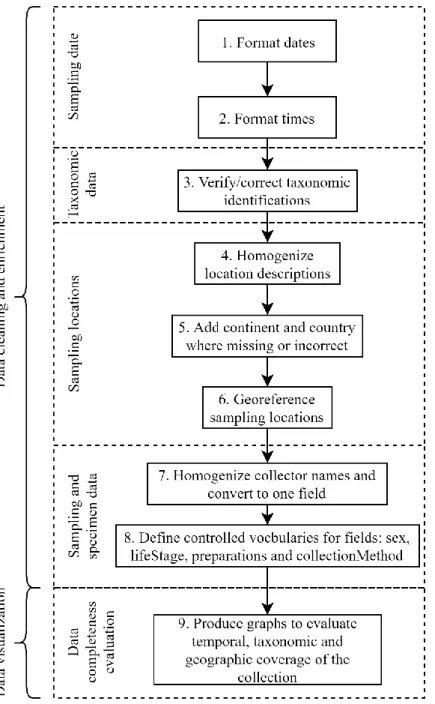
Figure 3.1 Steps employed in data cleaning and visualization for the MNHNC insect collection catalogue.

The methods used here (Figure 3.1) included a data cleaning process and then data completeness evaluation (i.e., information and taxonomic, temporal and geographic coverage of the collection) through visualization. The methods were applied as follows:

The first step of the data cleaning process was to format dates. The DarwinCore standard format best practice is defined to conform to the ISO 8601 international standard to represent date and time [37]. This format was used for the fields startDate, endDate and eventDate, and corresponds to “YYYY-MM-DD” for dates and “YYYY-MM-DD/YYYY-MM-“YYYY-MM-DD” for date intervals. The dataset included dates in various formats, such as “DD/MM/YY” and “(DD-DD)-MM-YYYY”. All of these formats were

(22)

17 identified and the Transform function of OpenRefine was used to change the dates to the correct format. To do this, regular expressions were constructed for each individual format using GREL. An example is shown below, to transform a string of format “(DD-DD)-MM-YYYY” to the format “YYYY-MM-DD/DD”.

if(isNotNull(value.match(/\([0-9]{2}-[0-9]{2}\)-[0-9]{2}-[0-9]{4}/)), slice(value,11,15) + "-" + slice(value,8,10) + "-" + slice(value,1,3) + "/" + slice(value,4,6), value)

For the field eventTime, the same method was used to format all entries according to the DarwinCore standard, which is “hh:mm”.

In order to confirm and correct taxonomic data, several steps were necessary. First, a list of canonical names was imported to OpenRefine and reconciled using the NCBI taxonomy standard service [38]. The reconciled names were verified individually to check for errors or incorrect matches, and the genera and/or specific epithets were updated where necessary. As a second verification step, the list of canonical names was imported into R [26], and the gnr_resolve function of the taxize package [35] was used to produce a list of corrected canonical names. For each canonical name, the corresponding Family and Order was obtained using the upstream function. The names that were different from the original were verified to check for errors. The resulting list was saved as a csv file and imported into Excel, where the VLOOKUP function was used to add the correct canonical name, Family and Order to matching records. For the geocoding process, the first step was to homogenize location descriptions. For this, the Cluster feature of OpenRefine was used. Key collision methods were used first for clustering, followed by the nearest neighbour method. For each method, all clusters corresponding to the same location described in different manners, with differences in punctuation, letter case, etc. were merged. The columns continent and country were reconciled against the Wikidata knowledge base to correct misspellings. After that, a csv file was created containing all individual locations that hadn’t been geocoded yet. For each individual location, columns for the country, state/province, island, county, municipality and locality were included. This file was imported into R using the read.csv function; for each location a string was created containing all existing information, and these were geocoded using the Google Maps API to obtain latitude and longitude. The resulting coordinates were then individually verified through the GEOLocate web application, to check if they corresponded to the correct location, and an uncertainty radius was attributed to each location. The csv file including location descriptions, coordinates and uncertainty radii was imported to Excel, where the VLOOKUP function was used to add coordinates and uncertainty to all the records sampled from each location.

The last cleaning step consisted in homogenizing the remaining fields and defining controlled vocabularies where possible. The collector field was represented by several columns, one for each collector name; the Cluster feature of OpenRefine was used to homogenize names known to be different representations but corresponding to the same collector throughout all columns, which were then concatenated using “|” as separator, to create the column recordedBy. For the fields sex, lifeStage, preparations and collectionMethod, controlled vocabularies were defined and used to replace all values. After cleaning and enriching the data, plots were produced using R to evaluate the completeness of the information and for a better visualization of the taxonomic, temporal and geographic coverage of the collection. All graphs were produced using the R graphics package [26], except the barplot with a gap produced to represent the countries where specimens were collected, for which the gap.barplot function of the plotrix package [39] was used.

(23)

18

3.3. Results

The dataset published on GBIF is available at https://www.gbif.org/dataset/79673413-746f-48f2-bd8a-7cf27807317e.The insect collection catalogue includes a total of 39 139 validated records, corresponding to a total of 79 885 specimens. Each record corresponds either to a single specimen or to a sample containing several specimens, collected at the same date and time, at the same location and by the same collector. The number of specimens for each record varies between 1 and 353.

A significant part of the collection was donated by private collectors. Only a small part of these donated collections was already catalogued. Of those that have been digitized and data integrated in the database, the Mendoça collection is the most well-represented in the collection catalogue, with 12 812 specimens recorded (16.0% of the total number of specimens). Other significant contributions are the collection donated by Teresa Pité, with 9897 specimens (12.4%), and the specimens collected in the EB network Biodiversity Stations (901 specimens, 1.1%) and by the Tagis – Butterfly Conservation Center (464 specimens, 0.6%).

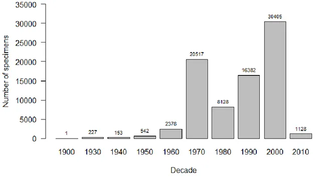
The specimens in the MNHNC collection were collected between 1905 and 2018. The number of specimens collected per decade is shown in Figure 3.2. The decades when most specimens were collected were 1970-1979 (20 517, 25.7% of total) and 2000-2009 (30 405, 38.1% of total).

Figure 3.2 Histogram of specimens of the MNHNC insect collection by decade of collection.

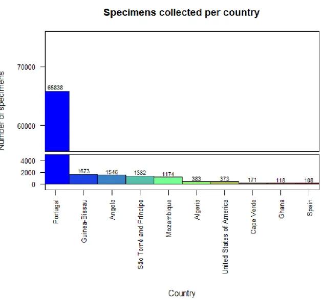
The number of specimens collected per country, for the countries represented by over 100 specimens in the collection, is shown in Figure 3.3. The large majority of the specimens were collected in Portugal (65 838, corresponding to 82.4% of all specimens). For other countries, the most represented ones are Guinea-Bissau, Angola, São Tomé and Príncipe and Mozambique (all ranging between 1000 and 2000 specimens). Of the 39 139 records, 27 746 (70.9% of total) are geocoded. Of these, 9 252 were geocoded during this work.

(24)

19

Figure 3.3 Bar graph of specimens of the MNHNC insect collection by sampling country. The plot includes the countries where 100 or more specimens were sampled.

Regarding the taxon rank to which specimens are identified (Figure 3.4 B), the majority are classified to the Species level (21 471, 26.9% of total) or to the Order level (49 824, 62.4% of total). Of the remaining specimens, 5313 (6.7%) are classified to the Family, 2757 (3.5%) to the Genus and 520 (0.7%) to the Subspecies.

The previous version of the MNHNC insect collection dataset was published on GBIF in 2014. The current version is more complete, includes more records and more detailed validated data. The version published in 2014 included a total of 30 535 records, corresponding to a total of 64 008 specimens. Of all records, 7916 (25.9%) were geocoded. In the new version of the dataset, the percentage of geocoded records increased to 70.9%. The percentage of specimens identified to each taxon rank in the dataset published in 2014 is shown in Figure 3.4 A. Thanks to the contribution of specialists, there was a significant increase in the percentage of specimens classified to the Species level (5.4% to 26.9%), along with a decrease in the percentage of specimens classified to the Order level (83.6% to 62.4%), meaning the taxonomic characterization of the collection is more complete in the current dataset.

(25)

20

Figure 3.5 illustrates the taxonomic coverage of the insect collection, represented as the number of specimens contained in the collection for the most well represented Orders (over 100 specimens). Diptera is the most represented Order in the collection, with 23 270 specimens (29.1% of total), followed by Coleoptera (16 886 specimens, 21.1% of total) and Hemiptera (14 327 specimens, 17.9% of total). Specimens belonging to the Class Entognatha, which includes the Orders Collembola, Diplura and Protura, are included in the insect collection, even though they do not belong to the Class Insecta. In fact the MNHNC collection includes specimens from the subphylum Hexapoda, which comprises both classes.

Figure 3.5 Bar graph of specimens of the MNHNC insect collection by Order. The plot includes the Orders represented by more than 100 specimens in the collection.

The number of specimens of each Family, for the Families represented by over 200 specimens in the collection, is shown in Figure 3.6. The most common Families in the collection are Drosophilidae (Order

A B

Figure 3.4 Percentage of specimens of the insect collection catalogue identified to each taxon rank, in the dataset published on GBIF in 2014 (A) and in the dataset published in 2019 (B). In (A), Class is omitted for clarity, accounting for 0.4% of specimens.

(26)

21 Diptera; 9985 specimens, 12.5% of total), Nymphalidae (Order Lepidoptera; 2166 specimens, 2.7%), Chrysomelidae (Order Coleoptera; 1533 specimens, 1.9%), Chironomidae (Order Diptera; 1453 specimens, 1.8%) and Pieridae (Order Lepidoptera; 1016 specimens, 1.3%).

Figure 3.6 Bar graph of specimens of the MNHNC insect collection by Family. The plot includes the Families represented by more than 200 specimens in the collection.

The MNHNC collection includes a total of 67 type specimens representing 42 species. Of these, 32 are holotypes, 5 are allotypes and 45 are paratypes.

(27)

22

3.4. Discussion

The main contribution of this work has been the overall quality improvement of the insect collection catalogue, as new data have been produced, such as many new geocoded records, improvement of existing data quality by data standardization and the publishing on GBIF of the improved dataset. In the current collection catalogue, all dates and times are standardized to the DarwinCore format. Fields such as collector name, sampling locality, life stage and preparation method have been standardized to a controlled vocabulary.

The new version of the dataset is more complete, both in terms of number of specimens (64 008 in 2014 vs. 79 885 in the current dataset) and in terms of geographic data available (25.9% of records geocoded in 2014 vs. 70.9% in the current dataset). During this work, taxonomic identifications were also verified and updated in cases of synonymy, meaning this data is more accurate. The use of specific tools for data cleaning, such as R and OpenRefine, allowed the data cleaning process to be done quickly and efficiently. After the dataset was complete, these tools were also used to visualize the data in terms of temporal, geographic and taxonomic coverage.

It is important to note that some of the donated collections already stored in the museum include more specimens, but a significant part of the data associated with them hasn’t been digitized or included in the catalogue yet, and so it wasn’t accounted for in the results presented here. Of these collections, the number of specimens yet to be digitized is estimated to be almost as much as the total number of specimens currently in the collection catalogue. The process of adding specimen data to the collection catalogue may be accomplished more quickly with the help of volunteers through a citizen science project, discussed in Section 4 of this work. There are also many specimens and samples in the museum that haven’t been screened, prepared or digitized yet. An important future work will be to continue these tasks as it is calculated that over 50% of the specimens in the MNHNC insect collection remain to be catalogued (L. F. Lopes personal communication). This will be an important contribution to biodiversity knowledge, making a significantly larger and more complete dataset available that can be used for research projects in different areas, such as species distribution modelling and studies of invasive species. As previously mentioned, NHC can represent species that are no longer possible to collect, for instance due to population reduction or extinction [2]. Therefore, it is, important to have these data, and preserved specimens, available for use when studying changes in biodiversity over time.

The MNHNC collection includes type specimens, which are of particular importance because they were used to describe a species, and therefore can be used as a comparison to identify other specimens. An important future work will be to exhaustively verify the data for these specimens in the dataset and document the type specimens in the collection.

(28)

23

4. Zooniverse project for data digitization

Citizen science, consisting of involving the general public in research, has been used for centuries in fields such as astronomy and meteorology. However, it has become more widespread in the last decades, with the development of online tools that facilitate the participation of volunteers. Online citizen science projects are most helpful for analysing or interpreting large amounts of data that require detection of patterns and anomalies unrecognized by computers [40]. They have been successfully used for purposes as diverse as designing self-assembling RNA molecules [41] and transcribing historical documents [42]. Currently, the most used tool for developing citizen science projects is Zooniverse (www.zooniverse.org), which has 1.7 million registered volunteers worldwide. It includes a free project builder platform which allows researchers to create projects quickly and at no cost [40].

One of the most time-consuming steps of NHC data digitization is the transcription of specimen data. Sampling information for most specimens is registered in labels, index cards and/or field notebooks, requiring transcription to a digital database. Several methods can be used to achieve this. One is having associated staff or volunteers transcribing each record individually from labels or paper records, which is time-consuming. An alternative is to use optical character recognition (OCR) software to transcribe data from photographs or scanned documents. This has proven useful for typewritten labels, but it is still not efficient for handwritten text [43, 44], which is the most common in NHC labels. Moreover, OCR can’t interpret or infer information, e.g. from abbreviations, and it doesn’t categorize the text into separate fields for collector, sampling location, sampling date, etc.

Citizen science projects have proven very useful for NHC specimen data transcription. They can be hosted on accessible online platforms where volunteers can transcribe data remotely from digitized representations of the labels or other paper records. Several institutions have developed platforms specifically for this purpose, such as DigiVol, developed by the Australian Museum and the Atlas of Living Australia [45], Les Herbonautes, of the French National Museum of Natural History [46], Notes from Nature, developed by the Natural History Museum in London, the Southeast Regional Network of Expertise and Collections organization, Calbug and the University of Colorado Museum [44], and the Smithsonian Transcription Center [47].

Besides being useful to reduce the time necessary to digitize NHC data, these platforms are also important tools for engaging scientific communication and education, since the volunteers learn more about the subjects of the projects as they participate. Citizen science projects involving data collection, such as species monitoring, increase the participant’s knowledge in the field [48]. For example, volunteers gathering data to monitor invasive plant species, showed increased awareness of invasive plants and their effects on ecosystems [49]. Data processing projects, such as transcription or image classification, are thought to raise public awareness to previously unknown fields of scientific research [48].

When provided with clear instructions or training, e.g. a tutorial on the structure of the records, volunteers can separate the different elements in the label (e.g. sampling date, location, the name of the collector, and taxonomic identification) in a way that cannot yet be done automatically. When the volunteers are fluent in the language the labels are written in, they can correct spelling errors and update location names that have changed since the sampling took place, given that information is easily available. Citizen science projects can also be used to enrich the information associated with the specimens, e.g. regarding damage to the specimen or morphological features, and even taxonomic determination data can be acquired from volunteers with expertise on the taxonomy of the target group [24].