Computing Changesets for RDF Views of Relational Data
Vânia M. P. Vidal!1, Narciso Arruda1, Matheus Cruz1, Marco A. Casanova2, CarlosBrito1, Valéria M. Pequeno3
1 Federal University of Ceará, Fortaleza, CE, Brazil
{vvidal, narciso, carlos}@lia.ufc.br, [email protected] 2 Department of Informatics – Pontifical Catholic University of Rio de Janeiro, RJ, Brazil
[email protected] INESC-ID, Porto Salvo, Portugal
Abstract. The Linked Data (LD) initiative fostered the publication of a large number of relational databases in the Linked Open Data (LOD) cloud. A gen-eral and flexible way of publishing relational data in RDF format is to create an RDF view of the underlying relational data (RDB-RDF view). An RDB-RDF view can be materialized to improve query performance and data availability. However, an RDB-RDF view must be continuously maintained to reflect dy-namic updates over the relational database. The contents of an RDB-RDF view, published on the LOD cloud, can also be fully or partially replicated by other LD applications to improve their efficiency. Thus, updates on an RDB-RDF view must be propagated to maintain other LD application views. This paper proposes a framework for the live synchronization of an RDB-RDF view. In the proposed framework, rules are responsible for computing and publishing the changeset required for the RDB-RDF view to stay synchronized with the rela-tional database. The computed changesets are then used for the incremental maintenance of the RDB_RDF views as well as application views. The paper also describes a strategy for automatically generating, based on a set of map-pings, the rules for computing the correct changesets for an RDB-RDF view. Finally, it suggests an architecture and describes an implementation and exper-iments to validate the proposed approach.
Keywords: RDF view ·View Maintenance · Linked Data · Relational database.
1
Introduction
There is a vast content of structured data available on the Web of Data as Linked Open Data (LOD). In fact, a large number of LOD datasets are RDF views defined on top of relational databases, called RDB-RDF views. The content of an RDB-RDF view can be materialized to improve query performance and data availability. How-ever, to be useful, a materialized RDB-RDF view must be continuously maintained to reflect dynamic source updates.
Furthermore, Linked Data applications, that consume data RDB-RDF view, can fully or partially replicate the contents of a materialized RDB-RDF view, by creating
RDF application views defined over the RDB-RDF view. The generation of RDF
application views improves the efficiency of applications that consume data from the LOD, and increases the flexibility of sharing information. However, the generation of RDF application views raises synchronization problems, since the original datasets can be continuously updated. Thus, updates on an RDB-RDF view must be propagat-ed to maintain the RDF application views.
A popular strategy used by large LOD datasets to maintain RDF application views is to compute and publish changesets, which indicate the difference between two states of the dataset. Applications can then download the changesets and synchonize their local replicas. For instance, DBpedia (http://wiki.dbpedia.org) and LinkedGe-oData (http://linkedgeodata.org/About) publish their changesets in a public folder.
This paper proposes a framework, based on rules, that provides live synchroniza-tion of RDB_RDF views. In the proposed framework (see Fig. 1), rules are responsi-ble for computing and publishing the changeset required for the RDB-RDF view to stay in synchronization with the relational database. The computed changesets are used by the synchronization tools for the incremental maintenance of RDB_RDF views and application views.
The use of rules is a very effective solution for computing changesets for RDB-RDF views [2,11]. However, creating rules that correctly compute changesets for RDB-RDF views can be a complex process, which calls for tools to automate the rule generation process. Another contribution of the paper is indeed a formal framework for automatically generating, based on a set of mappings, the rules for computing correct changesets for a wide class of RDB-RDF view. Our formalism allows us to precisely justify that the rules generated by the proposed approach correctly compute the changeset.
The remainder of this paper is organized as follows. Section 2 defines transfor-mation rules and correspondence assertions, the formalism used to specify a mapping between the relational schema and a target ontology. Section 3 introduces an abstract notation to define and materialize RDB-RDF views with the help of correspondence assertions. Section 4 describes a strategy, based on rules, for computing changesets for an RDB-RDF view. Section 5 summarizes related work. Section 6 covers an im-plementation and experiments. Section 7 presents the conclusions.
2
Mapping Relational Data to RDF
2.1 Basic Concepts and Notation
As usual, we denote a relation scheme as R[A1,....,An] and adopt mandatory (or not
null) attributes, keys, primary keys and foreign keys as relational constraints. In
par-ticular, we use F(R:L,S:K) to denote a foreign key, named F, where L and K are lists of attributes from R and S, respectively, with the same length. We also say that F
relates R and S.
A relational schema is a pair S=(R,Ω), where R is a set of relation schemes and Ω is a set of relational constraints such that: (i) Ω has a unique primary key for each relation scheme in R; (ii) Ω has a mandatory attribute constraint for each attribute
which is part of a key or primary key; (iii) if Ω has a foreign key of the form
F(R:L,S:K), then Ω also has a constraint indicating that K is the primary key of S. The
vocabulary of S is the set of relation names, attribute names, etc. used in S. Given a
relation scheme R[A1,....,An] and a tuple variable t over R, we use t.Ak to denote the
projection of t over Ak. We use selections over relation schemes, defined as usual. Let S=(R,Ω) be a relational schema and R and T be relation schemes of S. A list
ϕ = [F1,...,Fn-1] of foreign key names of S is a path from R to T iff there is a list
R1,...,Rn of relation schemes of S such that R1=R, Rn=T and Fi relates Ri and Ri+1. We say that tuples of R reference tuples of T through φ. A path φ is an association path iff
φ=[F1,F2], where the foreign keys are of the forms F1(R2:L2,R1:K1) and
F2(R2:M2,R3:K3).
We also recall a minimum set of concepts related to ontologies. A vocabulary V is a set of classes, object properties and datatype properties. An ontology is a pair
O=(V,Σ) such that V is a vocabulary and Σ is a finite set of formulae in V, the
con-straints of O. Among the concon-straints, we consider those that define the domain and range of a property, as well as cardinality constraints, defined in the usual way.
2.2 Transformation Rules
In this section, we briefly present a mapping formalism, based on rules, to transform instance data from a relational database to a target ontology vocabulary. Our formal-ism is much simpler than mapping languages such as R2RML [6], but it suffices to capture expressive mappings. Also, the formalism incorporates concrete domains to capture concrete functions, such as “string concatenation”, required for complex mappings, and concrete predicates, such as “less than”, to specify restrictions. Exam-ples of transformation rules will be presented in Table 4.
Let O=(V,Σ) be a target ontology and S=(R,Ω) be a relational schema, with vo-cabulary U. Let X be a set of scalar variables and T be a set of tuple variables, dis-joint from each-other and from V and U.
A literal is a range expression of the form R(r), where R is a relation name in U and r is a tuple variable in T, or a built-in predicate. A rule body B is a list of literals. When necessary, we use “B[x1,…,xk]” to indicate that the tuple or scalar variables
x1,…,xk occur in B. We also use “R(r), B[r, x1,…,xk]” to indicate that the rule body has a literal of the form R(r).
A transformation rule, or simply a rule, is an expression of one of the forms: • C(x) ← B[x], where C is a class in V and B[x] is a rule body
• P(x,y)← B[x,y], where P is a property and B[x,y] is a rule body.
We assume that the rules are not mutually recursive. Hence, they act as definitions of concepts in Vin terms of concepts in R. Indeed, we consider a transformation rule r as a short-hand notation the first-order sentence:
• ∀x1…∀xk ( C(x1) ⇔ B[x1…xk] ), if r is of the form C(x1) ← B[x1…xk], where
x1…xk are the variables that occur in B
• ∀x1…∀xk ( P(x1,x2) ⇔ B[x1…xk] ), if r is of the form P(x1,x2) ← B[x1…xk], where
x1…xk are the variables that occur in B.
Therefore, the mapping rules have a first-order semantics. In particular, we stress that the predicate function symbols have a fixed interpretation.
2.3 Correspondence Assertions
This section presents a more concise abstract syntax, based on correspondence asser-tions (CA) [12], for representing rules to transform data from a relational database to a target ontology vocabulary. The RDB-RDF views that we address are focused on schema-directed RDF publishing. As such, the correspondence assertions induce schema mappings defined by the class of projection-selection-equijoin queries, and support most types of data restructuring that are commonly found when transforming relational data to RDF. Moreover, the CAs suffice to capture all R2RML mapping patterns proposed in the literature which we are aware of [9].
Let S=(R,Ω) be a relational schema and O=(V,Σ) be an ontology. Assume that Σ has constraints defining the domain and range of each property. Briefly, there are three types of CAs (see Table 1):
• Class Correspondence Assertions (CCA), which map tuples of relations to instanc-es of classinstanc-es;
• Object Property Correspondence Assertions (OCA), which map relationships among tuples, through a path, to instances of object properties;
• Datatype Property Correspondence Assertions (DCA), which map values of attrib-utes to values of datatype properties.
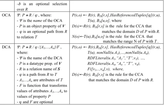
Table 1. Transformation Rules.
CA Notation Transformation Rule (TR)
CCA Ψ: C ≡ R[A1,...,An] δ, where:
- Ψ is the name of the CCA - R is a relation name of S, - A1,...,An are the attributes of the primary key of R, and
-δ is an optional selection over R
OCA Ψ: P ≡ R / ϕ , where: - Ψ is the name of the OCA - P is an object property of V - ϕ is an optional path from R to relation T
P(s,o) ← R(r), BD[r,s],HasReferencedTuples[ϕ](r,u),
T(u), BN[u,o], where
D(s)←R(r), BD[r,s] is the rule for the CCA that matches the domain D of P with R. N(o)←T(u),BN[u,o] is the rule for the CCA that matches the range N of P with T . DCA Ψ: P ≡ R / ϕ /{A1,...,An}/F ,
where:
- Ψ is the name of the DCA - P is a datatype prop. of V - R is a relation name of S - ϕ is a path from R to T - A1,...,An are attributes of T - F is function that transforms values of attributes A1,...,An to values of property P - ϕ and F are optional
P(s,o) ← R(r),BD[r,s], HasReferencedTuples[ϕ](r,u),
T(u), nonNull(u.A1),…,nonNull(u.An),
RDFLiteral(u.A1,“A1”,“T”,v1), …,
RDFLiteral(u.An,“An”,“T”, vn),
F([v1,..,vn],v), where,
D(s)←R(r), BD[r,s] is the rule for the CCA that matches the domain D of P with R.
Table 1 shows the formalism to express each type of CA and the transformation rules induced by the CA. The body of a rule induced by a CA Ψ is always an expres-sion of the form “R(r), B[r,x1,…,xk]”, where R is called the Pivot Relation of Ψ and r the pivot variable. Table 2 lists the definitions of the built-in predicates adopted.
A mapping between V and S is a set A of correspondence assertions such that: (i) If A has an OCA of the form P ≡ R/ϕ, where ϕ is a path from R to T, then A must
have a CCA that matches the domain of P with R and a CCA that matches the range of P with T.
(ii) If A has a DCA that matches a datatype property P in V with a relation name R of
S, then A must have a CCA that matches the domain of P with R.
To make the paper self-contained, we introduce an abstract notation to define
RDB-RDF views with the help of correspondence assertions.
Definition 1. An RDB-RDF view is a triple V = (OV, S, MV), where: • OV is the vocabulary of the view
• S is a source relational schema • MV is the mapping between V and S
Note that, by definition, since MV is the mapping between V and S, it satisfies con-ditions (i) and (ii) introduced in this section. The problem of generating the corre-spondence assertions is addressed in [11, 12] and is out of the scope of this work. In [12], we proposed an approach to automatically generate R2RML mappings, based on a set of correspondence assertions. The approach uses relational views as a middle layer, which facilitates the R2RML generation process and improves the maintainabil-ity and consistency of the mapping.
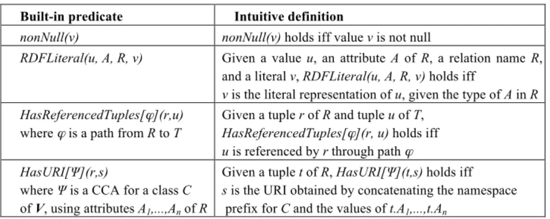
Table 2. Built-in predicates Built-in predicate Intuitive definition
nonNull(v) nonNull(v) holds iff value v is not null
RDFLiteral(u, A, R, v) Given a value u, an attribute A of R, a relation name R, and a literal v, RDFLiteral(u, A, R, v) holds iff
v is the literal representation of u, given the type of A in R HasReferencedTuples[ϕ](r,u)
where ϕ is a path from R to T
Given a tuple r of R and tuple u of T, HasReferencedTuples[ϕ](r, u) holds iff u is referenced by r through path ϕ HasURI[Ψ](r,s)
where Ψ is a CCA for a class C of V, using attributes A1,...,An of R
Given a tuple t of R, HasURI[Ψ](t,s) holds iff s is the URI obtained by concatenating the namespace prefix for C and the values of t.A1,...,t.An
2.4 Case Study: MusicBrainz_RDF View
MusicBrainz (http://musicbrainz.org/doc/about) is an open music encyclopedia that
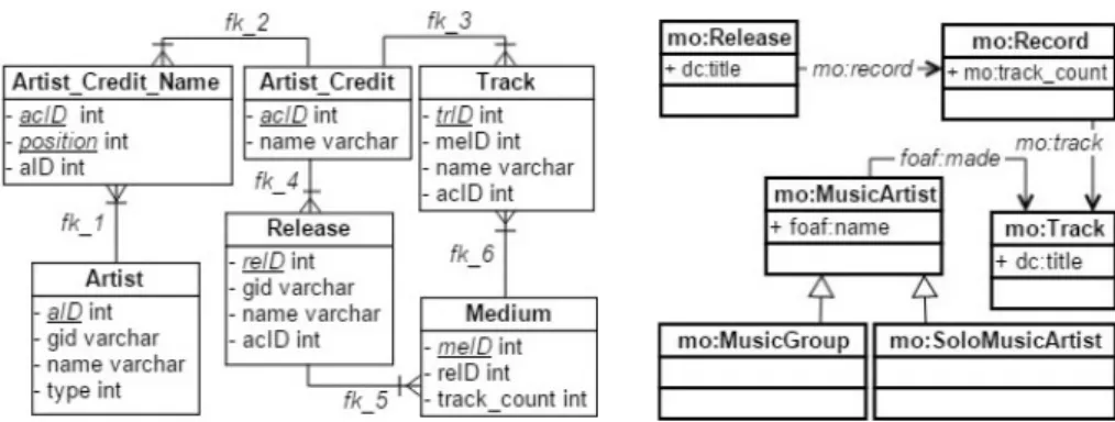
collects music metadata and makes it available to the public. The MusicBrainz Data-base is built on the PostgreSQL relational dataData-base engine and contains all of Mu-sicBrainz music metadata. This data includes information about artists, release groups, releases, recordings, works, and labels, as well as the many relationships be-tween them. Figure Fig. 2 depicts a fragment of the MusicBrainz relational database schema (for more information about the original scheme, see https://wiki.musicbrainz.org/MusicBrainz_Database/Schema. Each table has a distinct primary key, whose name ends with 'ID'. Artist, Medium, Release and Track represent the main concepts. Artist_Credit_Name represents an N:M relationship between Artist and Artist_Credit. The labels of the arcs, such as Fk_1, are the names of the foreign keys.
In our case study, we will use a RDB_RDF view, called MusicBrainz_RDF, which is defined over the relational schema in Fig. 2. Figure. 3 depicts the ontology used for publishing the MusicBrainz_RDF view. It reuses terms from three well-known vo-cabularies, FOAF (Friend of a Friend), MO (Music Ontology) and DC (Dublin Core). Table 3 shows a set of CAs that specifies a mapping between the relational schema in Figure 2, and the ontology in Figure 3, obtained with the help of the tool described in [12]. Table 4 shows the rules for CAs in Table 3 such that Artist is the pivot rela-tion (we omit the translarela-tions from attribute values to RDF literals for simplicity). The rules for the CAs in Table 4 specifies that each tuple r in Artist produces the follow-ing RDF triple:
• <http://musicbrainz.org/artist/r.gid> rdf:type mo:MusicArtist> (CCA1), where the URI http://musicbrainz.org/artist/t.gid is obtained as defined in Table 1. • <http://musicbrainz.org/artist/r.gid> foaf:name r.name. (DCA1)
• <http://musicbrainz.org/artist/t.gid> foaf:made
< http://musicbrainz.org/track/r*.trID, where r* is a tuple in Track such that r* is
The R2RML mappings, generated by the CAs in Table 3, are presented in [10].
Fig. 2. Fragment of MusicBrainz Schema Fig. 3. MusicBrainz_RDF View Ontology. Table 3. Correspondence Assertions.
CCA1 mo:MusicArtist ≡ Artist[gid]
CCA2 mo:SoloMusicArtist ≡ Artist[gid][type=1] CCA3 mo:MusicGroup ≡ Artist[gid][type=2] CCA4 mo:Record ≡ Medium[reID]
CCA5 mo:Track ≡ Track[trID] CCA6 mo:Release ≡ Release[gid]
OCA1 foaf:made ≡ Artist /[fk_1, fk_2, fk_3] OCA2 mo:track ≡ Medium / [fk_6]
OCA3 mo:record ≡ Release / [fk_5] DCA1 foaf:name ≡ Artist / name
DCA2 mo:track_count ≡ Medium / track_count DCA3 dc:title ≡ Track / name
DCA4 dc:title ≡ Release / name
Table 4. Transformation Rules for CCA1, OCA1 and DCA1. CCA1 mo:MusicArtist(s) ←artist(r), HasURI[CCA1](r, s)
OCA1 foaf:made(s,g) ←artist(r), HasURI[CCA1](r, s),
hasReferencedTuples[fk_1, fk_2, fk_3](r, f), hasURI[CCA5](f, g)
DCA1 foaf:name(s,v) ← artist(r), HasURI[CCA1](r, s), nonNull(r.name),
RDFLiteral(r.name,“name”, “artist”,v)
3
Materialization of RDB-RDF View
A materialization of an RDB_RDF view requires translating source data into the RDB_RDF view vocabulary as specified by the mapping rules. In the rest of this
pa-per, σS(t) denotes the state of S in time t, where S can be a source dataset, a relation or a RDB-RDF view.
In the following definitions, let V = (OV, S, MV) be an RDB-RDF view and t be a time value.
Definition 2. Let Ψ be a CA in MV, where R is the pivot relation of Ψ and T is the transformation rule induced by Ψ. Let r be a tuple in σR(t), and let T[r] be the trans-formation rule obtained by substituting the pivot tuple variable in the body of Tby tuple r. Ψ[r](t) is the set of triples that are produced by rule T[r] against σS(t). (See [10] for a detailed formal definition).
Definition 3 (RDF state of a tuple). Let r be a tuple in σR(t), where R is a relation in
S. The RDF state of tuple r w.r.t V at time t, denoted MV[r](t), is defined as: • MV[r](t) = {x / x is a triple in Ψ[r](t)}, if R is the pivot relation of a CA Ψ in MV • MV[r](t) = Ø, if R is not the pivot relation of any assertion Ψ in MV
Definition 4 (Materialization of V). The materialization or state of V at time t,
denot-ed MV(t) is defined as:
MV(t) = {x / x is a triple in MV[r](t), where r is a tuple in σR(t) and R is the pivot rela-tion of a CCA in MV}.
Referring to our case study, consider that the mappings defined by the CAs in Ta-ble 3. Suppose that current state of the relations in Fig. 2 is that shown in Fig. 4. TaTa-ble 5 shows the materialization or state of MUSICBRAINZ_RDF view for the current state of relations in Fig 4.
Fig. 4. State Example for Relations in Fig 2. Table 5. Materialization of MUSICBRAINZ_RDF MV(t0) = {
(mbz:ga1 rdf:type mo:MusicArtist); (mbz:ga1 foaf:name “Kungs”); (mbz:ga1 rdf:type mo:SoloMusicArtist); (mbz:ga2 rdf:type mo:MusicArtist); (mbz:ga2 foaf:name “Cookin’s on 3 B.”); (mbz:ga2 foaf:made mbz:t1);
(mbz:ga2 rdf:type mo:MusicGroup); (mbz:ga3 rdf:type mo:MusicArtist); (mbz:ga3 foaf:name “Kylie Auldist”);
(mbz:ga3 foaf:made mbz:t1);
(mbz:ga3 rdf:type mo:SoloMusicArtist); (mbz:m1 rdf:type mo:Record); (mbz:m1 mo:track_count 12); (mbz:m1 mo:track mbz:t1); (mbz:gr1 rdf:type mo:Release); (mbz:gr1 dc:title “Layers”); (mbz:gr1 mo:record mbz:m1); (mbz:t1 rdf:type mo:Track); (mbz:t1 dc:title “This Girl”)}
4
Computing Changesets for RDB-RDF Views
A changeset of an RDF dataset D from the state σD(t0) in time t0 to the state σD(t1) in time t1 is a pair <∆¯D(t0, t1), ∆+D(t0, t1)>, where:
σD(t1) = (σD(t0) − ∆¯D(t0, t1)) ∪ ∆+D(t0, t1). (1) In this section, we first formalize the problem of computing a changeset of an RDB-RDF view when updates occur in the source database. Then, we present a strat-egy, based on rules, for computing changeset for an RDB-RDF view.
4.1 Correct Changesets
Let V = (OV, S, MV) be an RDB-RDF view. Consider an update uS on a relation R of
S, and assume that uS is an insertion, a deletion or an update of a single tuple. Let t0 and t1 be the time immediately before and after the update uS, respectively.
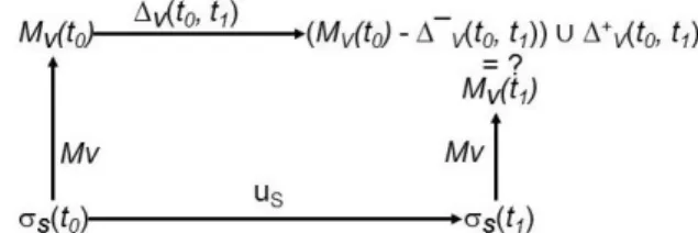
Fig. 5. The problem of computing RDB-RDF view changeset
Let σS(t0) and σS(t1) be the states of S respectively at t0 and t1, and let MV(t0) and
MV(t1) be the materialization of V respectively at t0 and t1.
A correct changeset for V is a changeset <∆¯V(t0, t1), ∆+V(t0, t1)> such that the ma-terialization of the RDB-RDF view V at time t1 satisfies (see the diagram in Fig. 5):
MV(t1) = (MV(t0) − ∆¯V(t0, t1)) ∪ ∆+V(t0, t1) (2)
4.2 A Strategy to Compute Correct Changesets
In this section, we present a strategy, based on rules, for computing correct changesets for an RDB-RDF view V = (OV, S, MV).
In our strategy, we first have to identify the relations in S that are relevant for V, that is, the relations whose updates might possibly affect the state of the view V, as in Definition 5 and Lemma 1 below.
Definition 5: Let R and R* be a relation in S. Let Ψ be a CA in MV. (i) R is relevant to Ψ iff R appears in the body rule of Ψ.
(ii) R is relevant for V iff R is relevant to some CA in MV.
In the rest of this section, let u be an update over S, and t0 and t1 be the time imme-diately before and after u, respectively.
Lemma 1: Let R be a relation in S. If R is not relevant to V, then MV(t0) = MV(t1). (Proof in [10]).
Thus, based on Lemma 1, we focus our attention only on the relations that are rele-vant for V. For each such relation R, we define triggers that are fired immediately before and immediately after an update on R, called before and after triggers, respec-tively, and which are such that:
BEFORE Trigger: computes the set ∆¯(t0, t1) using σS(t0) (database state BEFORE the update).
AFTER Trigger: computes the set ∆+(t0, t1) using σS(t1) (the database state AFTER the update).
From Definition 4, to materialize a RDB_RDF view, one has to compute the RDF state of the tuples in the pivot relations. The key idea of our strategy for computing the changesets is to re-materialize only the RDF_State of the tuples in the pivot rela-tions that might possibly be affected by the update. Thus, using ∆¯ and ∆+ one should be able to compute the new RDF state of the tuples that are relevant to the update. See Definitions 6 e 7, Lemma 2 and Theorem 1 in following.
Definition 6: Let Ψ be a CA in MV with path ϕ. Let R and R* be relations in S, where
R is relevant to R* w.r.t Ψ (Def. 5(iii)). A tuple r in σR(t) is relevant to a tuple r* in σR*(t) w.r.t Ψ iff r* references r through a not empty path ϕ*, where ϕ* is a prefix of ϕ.
For Definition 7 and Lemma 2, let u be an update on table R, and let t0 and t1 be the time immediately before and after u, respectively.
Definition 7: Let rnew and rold be the new and old state of the updated tuple in R. (i) ANEW= {r* / r* is a tuple in σR*(t0), where R is relevant to R* w.r.t a CA Ψ in MV
and ( r*=rnew or (rnew is relevant to r* w.r.t Ψ (Def. 6))}.
(ii) AOLD = {r* / r* is a tuple in σR*(t0), where R is relevant to R* w.r.t a CA Ψ in MV and ( r*=rold or (rold is relevant to r* w.r.t Ψ (Def. 6))}.
(iii) Let r* be a tuple in σR*(t0)∪σR*(t1). Then, r* is relevant to V w.r.t the update u iff
r* is in ANEW ∪ AOLD.
Lemma 2: Let r* be a tuple in σR*(t0)∪σR*(t1). If r* is not relevant to V w.r.t the up-date u (c.f Def. 8), then MV[r*](t0)=MV[r*](t1). (Proof in [10]).
Theorem 1: Let:
• u be an update on R
• t0 and t1 be the time immediately before and after u • rnew and rold be the new and old state of the updated tuple • ANEW and AOLD as in Definition 7(i) and 7(ii), respectively • ∆¯= {x / x is in MV[r](t0) where r is a tuple in ANEW ∪ AOLD } • ∆+= {x / x is in MV[r](t1) where r is a tuple in ANEW ∪ AOLD }
According to Lemma 2, an update may affect the RDF_State of a tuple in a pivot relation iff the tuple is relevant to V w.r.t the update (Def. 7(iii)). Fig. 6 shows the templates of the triggers associated with an update on a relation R. For example, con-sider u, the UPDATE on R were rold and rnew are the old and new state of the updated tuple, respectively. Before the update, Trigger (a) is fired, and the Procedure COMPUTE_ ∆¯[R] computes ∆¯ which contains the OLD RDF_State of the tuples that are relevant to V w.r.t update u (see Theorem 1). After the update, Trigger (b) is fired. Using the database state after the update, the Procedure COMPUTE_ ∆+[R] computes ∆+ which contains the new RDF_State of the tuples that are relevant to V w.r.t update u (see Theorem 1). It is important to notice, that the procedures COMPUTE_ ∆¯[R] and COMPUTE_ ∆+ [R] are automatically generated, at view definition time, based on the correspondence assertions of V. In [10] we show the algorithms which takes as input the set of correspondence assertions of V and compiles the procedures “COMPUTE_
∆¯[R]” and COMPUTE_ ∆+ [R].
Theorem 1 shows that the triggers in Figure 6 correctly compute the changesets for an update on a relation R. Triggers for insertions and deletions are similarly de-fined and are omitted here. A trigger for an insertion computes only ANEW, while a trigger for a deletion computes only AOLD (see Def. 7). Note that our strategy can be easily extended to more complex type of correspondence assertions, provided the sets
AOLD and ANEW are properly defined for more complex types of CA. BEFORE {UPDATE } 0N R THEN
∆¯ := COMPUTE_ ∆¯ [R] (rold, rnew ); ADD ∆¯ to changeset file of V.
(a)
AFTER {UPDATE} 0N R THEN ∆+ := COMPUTE_ ∆+ [R] (r
old, rnew ); ADD ∆+ to changeser file of V.
(b) Fig. 6. Triggers to compute changeset of V w.r.t. updates on R
4.3 Computing Changeset Example
To illustrate this strategy, consider that state of database in Fig. 4. Also consider u, the UPDATE on table Track were rold =<t1, m1, “This Girl”, ac2>, and rnew = <t1, m1, “This Girl (feat. Cookin' On 3 B.)”, ac1>. The changeset for the view
Mu-sicBrainz_RDF is computed in two phases as follow:
Phase 1: Executed by the BEFORE trigger (see Fig. 6(a)).
From Def. 6 e ACs in Table 3, we have:
- From OCA1: rold is relevant to tuples a2 and a3 in table Artist and rnew is relevant to tuples a1 and a2 in table Artist.
- From OCA2: rold and rnew are relevant to tuple m1 in Table Medium. From Def. 7, we have:
AOLD = {rold, a2, a3, m1>}.
ANEW = {rnew, a1, a2, m1>}. From Theorem 1, we have:
(mbz:ga2 rdf:type mo:MusicArtist); (mbz:ga2 foaf:name “Cookin’s on 3 B.”); (mbz:ga2 foaf:made mbz:t1);(mbz:ga2 rdf:type mo:MusicGroup);
(mbz:ga3 rdf:type mo:MusicArtist); (mbz:ga3 foaf:name “Kylie Auldist”); (mbz:ga3 foaf:made mbz:t1);(mbz:ga3 rdf:type mo:SoloMusicArtist); (mbz:m1 rdf:type mo:Record);
(mbz:m1 mo:track_count 12); (mbz:m1 mo:track mbz:t1);
(mbz:ga1 rdf:type mo:MusicArtist); (mbz:ga1 foaf:name “Kungs”); (mbz:ga1 rdf:type mo:SoloMusicArtist)}
Phase 2: Executed by the AFTER trigger (Fig. 6 (b)).
From Theorem 1, we have:
∆+ ={ (mbz:ga2 rdf:type mo:MusicArtist); (mbz:ga2 foaf:name “Cookin’s on 3 B.”); (mbz:ga2 foaf:made mbz:t1); (mbz:ga2 rdf:type mo:MusicGroup);
(mbz:ga3 rdf:type mo:MusicArtist); (mbz:ga3 foaf:name “Kylie Auldist”); (mbz:ga3 rdf:type mo:SoloMusicArtist);
(mbz:t1 rdf:type mo:Track);
(mbz:t1 dc:title “ThisGirl (feat. Cookin' On 3 B.)”); (mbz:m1 rdf:type mo:Record);
(mbz:m1 mo:track_count 12); (mbz:m1 mo:track mbz:t1);
(mbz:ga1 rdf:type mo:MusicArtist); (mbz:ga1 foaf:name “Kungs”); (mbz:ga1 foaf:made mbz:t1); (mbz:ga1 rdf:type mo:SoloMusicArtist)} Given VOLD, the old State of the MusicBrainz_RDF view in Table 5, in order to stay synchronized with the new state of database, the new state of the view can com-puted by: VNEW = (VOLD − ∆¯) ∪ ∆+.
5
Related Work
The Incremental View Maintenance problem has been extensively studied in the liter-ature for relational views [2], object-oriented views [8], semi-structured views [1], and XLM Views [3]. Despite their important contributions, none of these techniques can be directly applied to compute changesets for RDB-RDF views, since the com-plexity of the RDB-RDF mapping pose new challenges, when compared with other types of Views.
Comparatively less work addresses the problem of incremental maintenance of RDB-RDF views. Vidal et al. [11] proposed an incremental maintenance strategy, based on rules, for RDF views defined on top of relational data. Their approach was further modified and enhanced to compute changesets for RDB-RDF views. Although the approach in this paper uses similar formalism for specifying the view’s mappings, our strategy to compute changeset proposed in Section 4 differ considerably.
Endris at al [4] introduces an approach for interest-based RDF update propagation that can consistently maintain a full or partial replication of large LOD datasets. Fai-sal at al [5] presented an approach to deal with co-evolution which refers to mutual propagation of the changes between a replica and its origin dataset. Both approaches relies on the assumption that either the source dataset provides a tool to compute a
changeset at real-time or third party tools can be used for this purpose. Therefore, the contribution of this paper is complementary and rather relevant to satisfy their as-sumption.
Konstantinou et al [7] investigates the problem of incremental generation and stor-age of the RDF graph that is the result of exporting relational database contents. Their strategy required to annotate each generated triple with the mapping definition that generated it. In this case, when one of the source tuples change (i.e. a table appears to be modified), then the whole triples map definition will be executed for all tuples in the affected table. In contrast, using our rules we are able to identify which tuples are relevant to an update, and only the RDF_state of the relevant tuple are re-materialized. To the best of our knowledge, the computation of changeset for RDB-RDF views has not yet been addressed in any framework.
6
Implementation and Experiments
To test our strategy, we implemented the LinkedBrainz Live tool (LBL tool), which propagates the upadates over the MusicBrainz database (MBD database) to the LinkedMusicBrainz view (LMB View). The LMB View is intended to help Mu-sicBrainz (http://musicbrainz.org/doc/about) to publish its database as Linked Da-ta. Figure 1 depicts the general architecture of our framework, based on rules, for providing live synchronization of RDB_RDF views. The main components of the LBL tool are:
• Local MBD database: We installed a local replica of the MBD database available on January 24, 2017. The decompressed database dump has about 7 GB and was stored in PostgreSQL version 9.4.
• LMB View and Mappings: We created the R2RML mapping for translating
MBD data into the Music Ontology vocabulary (http://musicontology.com/),
which is used for publishing the LMB view. The LMB view was materialized using the D2RQ tool (http://www.d2rq.org/). It took 67 minutes to materialize the view with approximately 41.1 GB of NTriples. We also provided SPARQL endpoint for querying LMB View.
• Triggers: We created the triggers to implement the rules required to compute and publish the changesets, as discussed in Section 4.
• LBL update extractor: This component extracts updates from the replication file provided by MusicBrainz, every hour, which contains a sequential list of the up-date instructions processed by the MusicBrainz database. When there is a new rep-lication file, the updates should be extracted and then executed against the local of the MBD database.
• LBL Syncronization tool: This component enables the LMB View to stay synchro-nized with the MBD database. It simply downloads the changeset files sequential-ly, creates the appropriate INSERT/DELETE statement and executes it against the
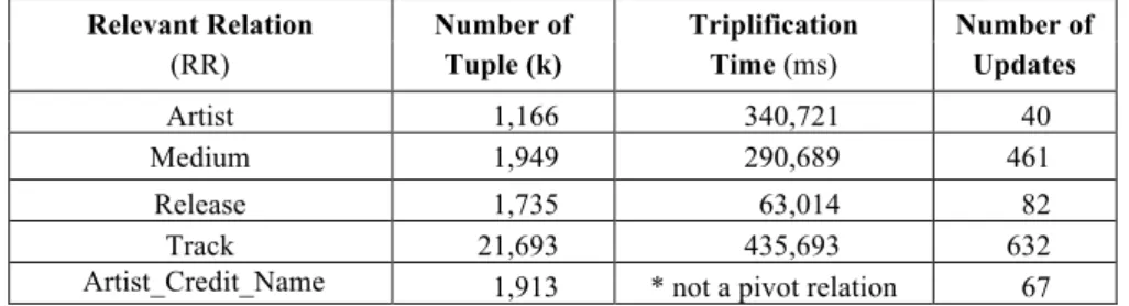
In our preliminary experiments, we measure the time to compute the changeset for replication file with sequential number 101758, which has 4,069 updates. The total time to compute the changeset for this replication file was 16 minutes. Table 6 and Table 7 summarize our experimental results, considering each relevant relation (RR) separately. Due to space limitation we show results only for updates over RR of case study in Section 2.4 (Artist, Medium, Release, track, and Artist_Credit_Name). • Table 6 shows: The total number of tuples in the RR, the total time (in
millisec-onds) spent to triplify the RR, and the total number of updates on the RR.
• Table 7 shows: The average number of tuples relevant to updates on the RR, and the average time (in milliseconds) to compute the changeset <∆¯, ∆+> for the RR. The experiments demonstrated that the runtime for computing the changeset is negligible, since the number of tuples that are relevant to an update is relatively small. We also analyzed the MusicBrainz replication file from one day and concluded that, in the experiments, just a small percentage of the tuples are relevant for the updates. Thus, we can conclude that, in the situation where the RDB_RDF view should be frequently updated, the incremental strategy far outperforms full re-materialization, and also the re-materialization of the affected tables [7].
Table 6. Relevant Relation of our Case Study (Fig. 2) Relevant Relation (RR) Number of Tuple (k) Triplification Time (ms) Number of Updates Artist 1,166 340,721 40 Medium 1,949 290,689 461 Release 1,735 63,014 82 Track 21,693 435,693 632
Artist_Credit_Name 1,913 * not a pivot relation 67 Table 7. Changeset Computation Performance for Relevant Relations Relevant Relation
(RR)
Avg Number of Relevant tuples
∆- (avg time)(ms) ∆+ (avg time)(ms)
i u i u Artist 1.47 66 119 10 13 Medium 4.15 76 36 7 8 Release 1.72 76 42 6 5 Track 4.23 121 495 49 321 Artist_Credit_Name 1 139 -- 16 --
7
Conclusions
In this paper, we presented a framework for providing live synchronization of an RDF view defined on top of relational database. In the proposed framework, rules are res-ponsible for computing and publishing the changeset required for the RDB-RDF view
to stay synchronized with the relational database. The computed changesets are used for the incremental maintenance of the RDB_RDF views as well as application views. We also presented a method for automatically generating, based on a set of corre-spondence assertions, the rules for computing the changesets for a wide class of RDB-RDF view. We showed that, based on view correspondence assertions, we can auto-matic and efficiently identify all relation that are relevant to a view. Using view corre-spondence assertions, we can also define how to identify the tuples that are relevant to a given source update. We provided a thorough formalization of our approach and indicated that the rules generated by the proposed approach correctly compute the changeset.
We also implemented the LinkedBrainz Live tool to validate the proposed frame-work. We are currently working on the development of a tool to automate the genera-tion of the rules for computing the changesets.
8
References
1. Abiteboul, S., McHugh, J., Rys, M., Vassalos, V., Wiener, J. L.: Incremental Maintenance for Materialized Views over Semistructured Data. In VLDB 1998, pp. 38–49 (1998) 2. Ceri, S. and Widom, J.: Deriving productions rules for incremental view maintenance. In
VLDB 1991, pp. 577–589 (1991)
3. Dimitrova, K., El-Sayed, M., Rundensteiner, E.A.: Order-sensitive View Maintenance of Materialized XQuery Views. In ER 2003, pp. 144–157 (2003)
4. Endris, K.M., Faisal, S., Orlandi, F., Auer, S., Scerri, S.: Interest-based RDF update prop-agation. In: 14th International Semantic Web Conference - ISWC2015 (2015)
5. Faisal, S., Endris, K.M., Shekarpour, S., Auer, S.: Co-evolution of RDF Datasets. In: 16th International Conference – ICWE 2016 (2016)
6. Hert, M., Reif, G., Gall, H.: A comparison of RDB-to-RDF mapping languages. In I-Semantics'11, ACM (2011)
7. Konstantinou, N., Spanos, D.E., Kouis, D., Mitrou, N.: An approach for the incremental export of relational databases into rdf graphs. International Journal on Artificial Intelli- gence Tools 24(2), 1540,013 (2015)
8. Kuno, H. A. and Rundensteiner, E. A.: Incremental Maintenance of Materialized Object-Oriented Views in MultiView: Strategies and Performance Evaluation. In IEEE TDKE, vol. 10, no. 5, pp. 768–792 (1998)
9. Sequeda, J., Priyatna, F., Villazón-Terrazas, B.: Relational Database to RDF Mapping Pat-terns. In: Workshop on Ontology Patterns (WOP2012), Boston, USA, 2012
10. Vidal, V.M.P., Arruda, N., Casanova, M.A., Brito, C., Pequeno, V.M.: Computing Chang-esets for RDF Views of Relational Data. Technical Report, Federal University of Ceara (2016). Available at http://tiny.cc/TechnicalReportUFC2017
11. Vidal, V.M.P., Casanova, M.A., Cardoso, D.S.: Incremental Maintenance of RDF Views of Relational Data. In ODBASE 2013, pp 572-587 (2013)
12. Vidal, V.M.P., Casanova, M.A., Eufrasio, L., Monteiro, J.M.: A semi-automatic approach for generating customized R2RML mappings. In SAC'14. ACM, pp.316-322. (2014)