F
ACULDADE DEE
NGENHARIA DAU
NIVERSIDADE DOP
ORTOA data mining approach to predict
probabilities of football matches
Tiago Filipe Mendes Neves
Mestrado Integrado em Engenharia Electrotécnica e de Computadores Supervisor: João Mendes Moreira
A data mining approach to predict probabilities of
football matches
Tiago Filipe Mendes Neves
Mestrado Integrado em Engenharia Electrotécnica e de Computadores
Abstract
One of the reasons for football being the most popular sport in the planet is its unpredictability. Every day, fans around the world argue over which team is going to win the next game or the next competition. Many of these fans also put their money where their mouths are, by betting large sums on their predictions.
Due to the large amount of factors that can influence the outcome of a football match, it is incredibly difficult to correctly predict its probabilities. With the increasing growth of the amount of money invested in sports betting markets it is important to verify how far the machine learning techniques can bring value to this area. To solve this problem we propose building data-driven solutions designed through a data mining process. The data mining process allows us to build models that can give us predictions according to the data that we feed them.
In this thesis we study how does machine learning algorithms, in the context of data mining, perform when predicting football matches. The problem was approached from several ways: from the classification point of view, analyzing the problem in terms of accuracy, and from the point of view of classification probabilities, analyzing if the calculated probabilities are able to beat the bookmakers.
Following the CRISP-DM methodology, we started by formulating the problem and under-standing the tools that were available. After we proceeded with the data acquisition and cleaning phase, gathering data from several sources and storing it in a database. The following step in-volved getting more familiar with the data, focusing on the exploratory data analysis. From the extracted knowledge we explored how features could be generated and analyzed how to select only the relevant. We then tested several base-learners such as decision trees, k-nearest neighbors and neural networks, followed by several ensemble techniques in order to improve the results. At last, we validated the results obtained in a full season and attempted some techniques in order to verify how the results could be improved.
Keywords: Sports predictions, data mining, machine learning, ensemble learning
Resumo
Uma das razões pela qual o futebol é considerado o desporto mais popular do planeta é a sua imprevisibilidade. Todos os dias, em todo o mundo, os adeptos debatem sobre que equipa vai ganhar o próximo jogo ou a próxima competição. Muitos destes adeptos acabam por apostar largas quantias nas suas previsões.
Devido a um grande número de factores que podem influenciar o resultado de um jogo de fute-bol, é incrivelmente difícil prever as probabilidades correctamente. Com o crescimento cada vez mais acentuado de dinheiro investido na área de apostas desportivas, torna-se importante perce-ber até onde os algoritmos de aprendizagem computacional podem trazer valor à área. Para re-solver este problema, propomo-nos a construir soluções baseadas em dados, através do processo de mineração de dados. O processo de mineração de dados permite-nos construir modelos que nos conseguem prever as probabilidades com base nos dados que lhe fornecemos.
Nesta tese estudamos qual é a performance dos algoritmos de aprendizagem computacional, no contexto de mineração de dados, para prever jogos de futebol. O problema foi abordado de duas formas diferentes: analisando do ponto de vista de um problema de classificação, isto é, analisar o problema em termos de exatidão da previsão do favorito, e do ponto de vista de probabilidades de classificação, analisando se as probabilidades dos modelos são capazes de ter lucro contra as casas de apostas.
Seguimos a metodologia de CRISP-DM, onde começamos por formular o problema e perceber as ferramentas disponíveis. Após isso, procedemos à fase de angariação e de limpeza de dados, juntando várias fontes e criando uma base de dados. O passo seguinte envolveu a familiarização com os dados, focando-se no processo de exploração e análise dos dados. Do conhecimento ex-traído foi explorado como é que se poderia gerar features e posteriormente selecionar apenas as relevantes. Testamos depois vários base-learners, nomeadamente árvores de decisão, k-vizinhos mais próximos e redes neuronais. Posteriormente avaliamos vários métodos de ensemble na tenta-tiva de melhorar os modelos. Por fim, validou-se os resultados na temporada mais recente presente nos dados e tentaram-se técnicas com vista à melhoria dos resultados.
Agradecimentos
Gostaria de agradecer em primeiro lugar ao meu orientador de tese, prof. Dr João Mendes Moreira, por me ter dado esta oportunidade de explorar este tópico pelo qual sou apaixonado, e por sempre me orientar na direção certa. Um breve agradecimento a todos os professores que me educaram ao longo dos anos.
Um agradecimento a todos os meus amigos, em especial para o que eu conheci no primeiro dia do meu 1o ano, para o que conseguiu entrar na tropa apesar de ser um grande trapalhão, para o que consegue arranjar tempo para estudar medicina e ser empreendedor de caracóis, para o que foi merecidamente banido no League of Legends e para o que tem um estilo de vida contrário ao meu mas com o qual formei uma excelente equipa nos últimos 5 anos.
Quero agradecer ao meu irmão pelo conhecimento e conselhos que me fornece e à minha avó por ter sido a minha mãe quando a minha mãe não lhe era possível ser.
Por fim, quero agradecer à minha mãe, que fez do seu objectivo de vida a educação dos seus filhos. Objectivo que agora é um sucesso.
Tiago Neves
Contents
1 Introduction 1
1.1 Context . . . 1
1.2 Goals . . . 2
1.3 Methodology . . . 2
1.3.1 Phase one: business understanding . . . 2
1.3.2 Phase two: data understanding . . . 3
1.3.3 Phase three: data preparation . . . 3
1.3.4 Phase four: modeling . . . 3
1.3.5 Phase five: evaluation . . . 3
1.3.6 Phase six: deploy . . . 4
1.4 Thesis structure . . . 4
2 Betting mathematics 5 2.1 Interchanging probabilities and odds . . . 5
2.2 Law of large numbers . . . 5
2.3 Bookmakers and betting exchanges . . . 6
2.4 The odds . . . 6
2.4.1 How are initial odds calculated . . . 6
2.4.2 How are odds balanced . . . 7
2.5 Value betting . . . 7
3 Data mining concepts and techniques 9 3.1 Data pre-processing . . . 9 3.1.1 Curse of dimensionality . . . 9 3.2 Feature generation . . . 11 3.3 Feature selection . . . 11 3.3.1 Filter methods . . . 11 3.3.2 Wrappers . . . 12
3.3.3 Built-in methods: random forest . . . 13
3.4 Machine Learning . . . 13
3.4.1 Data mining tasks . . . 14
3.4.2 Classification . . . 14 3.5 Algorithms . . . 15 3.5.1 Decision trees . . . 15 3.5.2 k-nearest neighbor . . . 16 3.5.3 Neural networks . . . 17 3.6 Evaluation metrics . . . 19 3.6.1 Accuracy . . . 19 vii
viii CONTENTS
3.6.2 Profit (Rentability) . . . 19
3.6.3 Return on investment (ROI) . . . 19
3.6.4 Difference between real profit and expected profit . . . 20
3.6.5 Ranked probability score . . . 20
4 Ensemble learning 21 4.1 The generalization problem . . . 21
4.2 Bias and Variance . . . 21
4.2.1 Bias . . . 21
4.2.2 Variance . . . 22
4.2.3 Bias-Variance trade-off . . . 23
4.3 Scenario: Decision trees parameter optimization . . . 23
4.4 Regularization . . . 24
4.5 Ensemble . . . 25
4.5.1 Bagging and Subsampling . . . 25
4.5.2 Boosting . . . 26
4.6 Ensembling decision trees . . . 27
4.6.1 Bagging and AdaBoost . . . 27
4.6.2 Random forest . . . 27
4.6.3 Gradient boosting . . . 27
4.7 Ensembling neural networks . . . 28
4.7.1 Bagging and boosting . . . 28
4.7.2 Negative correlation learning . . . 28
5 Data mining in the sports context 29 6 The approach to the problem and results 33 6.1 Business understanding . . . 33
6.1.1 Determine the business objectives . . . 33
6.1.2 Determine the data mining goals . . . 34
6.1.3 Assess the situation . . . 34
6.1.4 Evaluation metrics . . . 35
6.2 Data understanding . . . 36
6.2.1 Collect the initial data . . . 36
6.2.2 The used data . . . 36
6.2.3 Explore the data . . . 37
6.3 Data preparation . . . 39 6.3.1 Train/test/validation split . . . 39 6.3.2 Generation of features . . . 39 6.3.3 Selection of features . . . 41 6.4 Modeling . . . 44 6.4.1 Tree-based models . . . 44 6.4.2 Distance-based models . . . 49 6.4.3 Neural networks . . . 50
6.5 A survey of the state-of-the-art algorithms . . . 56
6.6 Result optimization . . . 58
6.6.1 Intra-league testing . . . 58
6.6.2 Intra-season training . . . 59
CONTENTS ix
7 Conclusions 61
7.1 Future work . . . 62
A The expected goals metric 63
B Exploratory data analysis 65
B.1 The correlation matrix . . . 65
B.2 Goals . . . 67
B.3 Shot-based variables . . . 70
C football-data.co.uk data 73
D fivethirtyeight.com data 75
E Comparing state-of-the-art neural network ensemble methods in football predictions 77
List of Figures
1.1 Predicted growth of the gambling market in the European Union. . . 1
2.1 An example of how betting with a positive expected value yields profit in the long term. . . 8
3.1 Visualization of the increased dimensionality. . . 10
3.2 Visualization of the Hughes Phenomenon. . . 10
3.3 A visualization of the different ranges of correlation with the target label. . . 12
3.4 A visualization of an example of the feature importance in the random forest. . . 13
3.5 A example decision tree classifying if a person should or not play badminton. . . 15
3.6 A example of a k-nearest neighbor classification. . . 16
3.7 Basic architecture of the perceptron. . . 17
3.8 A visualization of a neural network. . . 18
4.1 Representation of the bias-variance problem as an analogy to the precision-accuracy. 22 4.2 Representation of how bias, variance and overall error moves according to the model complexity. . . 23
4.3 Movement of the Bias-Variance trade-off according to the model complexity. . . 24
4.4 Production of subsamples in bagging. . . 25
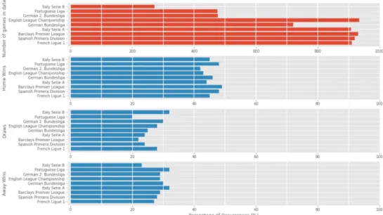
6.1 Analysis of the distribution of the final results of football matches according to the league. . . 38
6.2 Accuracy of the random forest classifier model with 1000 estimators according to the number of instances used for training. . . 38
6.3 Percentage of correct predictions by the bookmakers across the different leagues. 41 6.4 Performance of the top k features in feature importance tested on a random forest classifier with 1000 estimators. . . 44
6.5 Optimal hyperparameter (max_depth) search in the decision tree classifier. . . 45
6.6 Optimal hyperparameter (k) search in the k-nearest neighbor. . . 49
6.7 Optimal hyperparameter (network architecture) search for neural networks. . . . 51
6.8 Average results of the best performing models in the test set. . . 56
6.9 Average results of the best performing models in the validation set. . . 57
6.10 Average results of the tests in separated leagues. . . 58
6.11 Average results of the validation tests in a smaller validation set. . . 59
6.12 Probability distribution of the models home team predictions. . . 60
A.1 Visualization of the expected goals from the different areas of the pitch. . . 63
A.2 Visualization of the expected goals from Bruno Fernandes shots in the 18-19 season. 64
xii LIST OF FIGURES
B.1 Correlation matrix from all variables. . . 65
B.2 Correlation matrix from all variables, filtered to only show correlations above 0.4. 66 B.3 Histogram of the number of goals scored by a team in a match. . . 67
B.4 Histogram of the number of goals scored by both teams in a match. . . 68
B.5 Histogram of the number of goals scored by both teams in a match, separated by league. . . 69
B.6 Histogram of the number of shots by a team in a match. . . 70
B.7 Histogram of the number of shots on target by a team in a match. . . 70
B.8 Histogram of the difference of shots in a match. . . 71
B.9 Histogram of the difference of shots on target in a match. . . 71
B.10 Histogram of the number of corners by a team in a match. . . 72
B.11 Histogram of the number of expected goals by a team in a match. . . 72
C.1 A sample of the football-data.co.uk data. . . 73
List of Tables
5.1 A brief summary of the literature review. . . 31
6.1 Subsets generated from the data set. . . 39
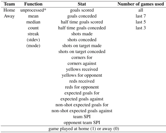
6.2 A collection of the features generated. . . 40
6.3 Baseline model performance. . . 41
6.4 Results of the different feature sets on a random forest classifier with 1000 esti-mators. . . 42
6.5 Results of the different feature sets on a k-nearest neighbor classifier with k = 5. . 42
6.6 Results of the different correlation filtered feature sets on random forest classifier with 1000 estimators. . . 43
6.7 Average results of 100 runs of the decision tree classifier with sklearn’s default parameters. . . 44
6.8 Average results of 100 runs of the decision tree classifier predictions on the test set. 46 6.9 Average results of 50 runs of decision tree ensembles (bagging and AdaBoost) in the test set, using 50 estimators. . . 46
6.10 Average results of 10 runs of decision tree bagging ensemble in the test set, using 1000 estimators. . . 47
6.11 Average results of 50 runs of random forest classifier in the test set, using 50 estimators. . . 47
6.12 Average results of 10 runs of random forest classifier in the test set, using 1000 estimators. . . 48
6.13 Average results of 50 runs of both gradient boosting techniques in the test set, using 50 estimators. . . 48
6.14 Results of a single run of the k-nearest neighbors in the test set. . . 49
6.15 Average results of 50 runs of the bagging with k-nearest neighbors classifiers in the test set, using 50 estimators. . . 50
6.16 Average results of 50 runs of the neural networks in the test set. . . 51
6.17 Average results of 50 runs of the neural networks ensemble techniques in the test set (without early stopping). . . 53
6.18 Average results of 50 runs of the neural networks ensemble techniques in the test set using early stopping. . . 54
6.19 Average results of 50 runs of the negative correlation learning algorithm, with lambda = 0.2, in the test set. . . 55
Abbreviations
BN Bayesian Network
CRISP-DM CRoss Industry Standard Process for Data Mining
k-NN k-Nearest Neighbor
NN Neural Network
PCA Principal Component Analysis
ROI Return on investment
sklearn scikit-learn
SPI Soccer Power Index
Chapter 1
Introduction
1.1
Context
Gambling was always an interesting concept to human beings. If we ask a person if they would trade e1 for e0.95 they would immediately reject the proposal. Being guaranteed to lose money is something that is not usually accepted without being rewarded. In betting, the reward comes from the existing probability of winning money. Even though in the long term more money is lost than won, the human brain is blinded by the prospect of a big win.
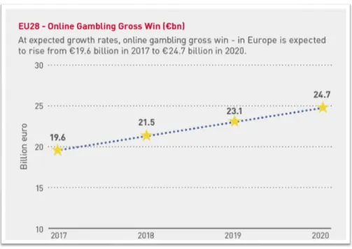
For many reasons, including sports being one of the main forms of entertainment in the world, online gambling is growing, as can be seen in the figure1.1. And with growing markets, opportu-nities to explore it arise.
Figure 1.1: Predicted growth of the gambling market in the European Union. SourceEGBA(2018)
2 Introduction
There is a niche part of gambling that is of interest to us: football betting. Unlike other forms of gambling, in football betting, the probabilities are not easily calculated or predefined. When we make a bet in roulette or in blackjack we can know the probabilities a priori, being easily calculable with probabilistic theory. This is not possible in football.
In a complex game such as football, it is also very complex to predict the games. Each game requires specialists opinion and complex models in order to set the initial probabilities. And then there is also an ability for the market to self regulate in a way that the bookmakers make the same profit regardless of the outcome.
With so many factors to take into account when calculating these probabilities, there is the possibility that errors or misjudgments occur. These can be taken advantage of by bettors: if the bookmaker is paying a price that is higher than what the real probability, by the law of large numbers, the bettors will make money in the long term.
1.2
Goals
The goal of the thesis is to evaluate how machine learning models perform in football match predictions, both in accuracy and probability-based approaches, with a special focus on evaluating if models can have the ability to make a profit. The question that we are trying to answer is: how do the predicted probabilities done by machine learning algorithms compare to the bookmakers’ predicted probabilities.
There is a need to verify where the state of the art machine learning algorithms stand: are they unable to make correct predictions, getting constantly outsmarted by the market, or are they able to see patterns in data which the human eye can not see and extract profit out of that information.
1.3
Methodology
The methodology that was used in the development of this thesis was based on the CRISP-DM (CRoss Industry Standard Process for Data Mining), with some added details from agile method-ologies, as for example, a backlog and prioritization of tasks with the most value associated. The phases of the CRISP-DM methodology follow next.
1.3.1 Phase one: business understanding
As considered by many, including the authorShearer(2000), this is the most important phase of the data mining project. Here we need to understand the objectives from the business perspective, define the data mining problem to solve and then develop a plan in order to achieve the objectives. Business understanding involves key steps such as determining business objectives, assessing the situation, determining the data mining goals and producing the project plan.
1.3 Methodology 3
1.3.2 Phase two: data understanding
This phase (Shearer,2000) starts with an initial data collection, followed by getting familiar with the data, identify data quality problems, discover initial insights into the data and/or detect inter-esting subsets.
It is crucial that the analyst understands the data that he has at its disposal: it guarantees that the following processes have a solid foundation since all the following processes are dependent on what we are able to extract from data. Making sure that the data is fully understood also makes sure that the best obtainable solution is achievable: if some part of the data is misinterpreted or ignored it might lead to models with sub-par performance.
1.3.3 Phase three: data preparation
It covers the construction of the final data set, that will later be fed into the models. The five steps in data preparation (Shearer,2000) are the selection, cleaning, construction, integration, and formatting of data.
Since models learn from the data that they are fed with it is very important to make sure that the data that goes into training the models is within certain standards, such as being clean from defective samples and misread values.
Cleaning data is then essential and that means making sure that the various data sources are gathered together without creating more problems in the data, that missing values are correctly handled and the data is in the correct format.
The great majority of problems also require that the initial data is transformed into features that are relevant to the problem that we are trying to predict. In our scenario, we need to transform the data from the matches that the teams play into variables that quantify the strength of the team in individual areas of play in order to be able to compare them.
1.3.4 Phase four: modeling
This phase (Shearer,2000) is where modeling techniques are selected and applied, calibrating their parameters to optimal values.
This is the step where we build the models with the available data and then assess the model performance. This step might require that we go back to the previous phase in order to reshape the data to improve our models since they are heavily reliant on the data that we feed them.
1.3.5 Phase five: evaluation
Before deploying the models it is important to validate and review the way the model was built in order to assure that a faulty model that does not meet the business criteria is not deployed. In this phase (Shearer,2000), the key steps are the evaluation of results, the review process and the determination of the next steps.
4 Introduction
1.3.6 Phase six: deploy
The creation of the model does not end the data mining process. In this step is where we enter the production phase. It is needed to develop a way to present the knowledge that the models found, which is dependent on the final target and business goal.
1.4
Thesis structure
The remainder of this thesis is organized as follows:
• Chapter 2 introduces mathematical concepts related to betting.
• Chapter 3 is a brief overview of key data mining concepts, with a focus on the data prepara-tion phase.
• Chapter 4 reviews some machine learning algorithms, focusing on the classification algo-rithms that have the ability to generate probabilities.
• Chapter 5 goes in-depth into ensemble learning, explaining the problem that is solved with ensembles and introducing algorithms for decision trees and neural networks.
• Chapter 6 briefly reviews previous work in the area of sports and football match predictions. • Chapter 7 describes the methodology, presents the results and conclusions of the experiences
that were conducted in order to predict football matches.
• Chapter 8 summarizes the work done and reflects on the obtained results. At last, future research ideas are pointed out.
Chapter 2
Betting mathematics
The knowledge of some key components of the math behind the betting process is crucial in order to understand the problem.
In this chapter, we describe key formulas and concepts of betting mathematics. First, we define what is an odd and the law of large numbers. Then we go more in-depth with the betting options that exist. Following that, there is an explanation of how the odds are set. At last, the concept of value betting, which allows us to profit from betting, is described.
2.1
Interchanging probabilities and odds
decimal odds= 1
probability o f the outcome (2.1)
The importance of the equation2.1for betting is similar to Ohm’s Law for circuit analysis or Newton’s Laws of Motion for physics.
It allows us to interchange the fair price and probability of the outcome. We can, given an expected probability, calculate the expected price and based on it verify whether it is worth to bet or not.
2.2
Law of large numbers
The understanding of this concept is crucial in order to comprehend how to make a profit when betting. This law implies that the average value of a large number of events converges to the expected value.
This is crucial since the majority of bets end in binary situations: either you win or lose, which means that you do not have smooth, continuous changes in the balance. Changes are abrupt and discrete, which means that because of their random nature we need to test them in the long-term and not in short-term results.
6 Betting mathematics
2.3
Bookmakers and betting exchanges
There are two ways of betting:
• In bookmakers, that is, companies that allow us to bet against their odds. The bookmaker defines the odds and regulates them as they wish.
• In betting exchanges, we can buy and sell bets as if they were stocks, by defining the price and amounts that we want to sell/buy from the market. The exchange works as an interme-diate that matches the bets from the costumers with each other, which means that the clients bet against each other.
At first sight, they might leave the impression that they are essentially the same, but when it comes to taxing their clients they have very different approaches.
On the bookmakers they introduce their taxes in the odds offered to the clients. That means that if we sum the probabilities of every outcome of a certain event it will result in a probability over 100%. Their business relies on you constantly placing bets and by complying with their system you will lose money in the long term. The value that you are expected to lose per unit you bet varies from bookmaker to bookmaker and from market to market, but it ranges from 3% to more than 18%. This type of taxation is equivalent to paying VAT when buying a product.
In contrast, betting exchanges work differently. They work by taxing our profits. That makes it possible to have fair odds, that is, where the sum of probabilities for every outcome is 100%. In exchange, you pay a tax when you withdraw your funds. The analogy that can be made is the way that the state taxes companies profits.
2.4
The odds
The odds that are offered have their cycle of life. They have a starting point and the live their life following a set of rules that allows bookmakers to maximize their profit and they die when the event starts.
2.4.1 How are initial odds calculated
In betting exchanges the initial odds are simply set by the bettors themselves, having their own criteria to define what they think is the correct price. Then, the gathering of their opinions define the odds, essentially wisdom of the crowd.
For bookmakers, as they do not have this system that has this ability to set the odds, they need to have a team of specialists on predictions that set an initial price. After that, they release the calculated probabilities to the market, but they take a larger than usual margin for themselves, al-lowing them to not lose much when mistakes happen. Then they gradually decrease their margins, increasing the odds until bettors start to place bets on the outcomes. With models becoming more reliable, the starting margins are getting lower.
2.5 Value betting 7
2.4.2 How are odds balanced
The bookmaker’s goal is to make a profit. The main goal in each match is to maximize their profit. For this to happen, the odds move in a way so that the profit of the bookmakers will always be the same, regardless of the outcome. This allows the bookmakers to reduce variability in their results. That means that when there is a lot of money being placed in one of the outcomes, the odds of the back (outcome to happen) will be lowered and the odds of the lay (outcome not to happen) will be increased.
As the price of the back of the outcome is lowered and the price to lay the outcome is higher, the bettors will be more tempted to put money in the lay bet than before since now its value is higher. This will balance the distribution of profits across all outcomes and the bookmaker will have the same profit independently of the outcome. This is the way that bookmakers have to guarantee that they maximize their profits, regardless of the outcome.
2.5
Value betting
The way to make a profit in the betting market is simple. If we consistently bet in odds that represent a lower probability than the real probability of the outcome, we will have an expected value, defined in equations2.2and2.3, over 1. This means that it is expected to earn more than what was invested. By the law of large numbers, in the long-term, the return of a large number of bets will be approximately the same as the expected value.
expected value= probability(outcome)∗ odd(outcome) (2.2)
expected value= probability(outcome)
bookmakers probability(outcome) (2.3)
We call a bet on which the real probability of the outcome is higher than what the bookmakers pays us a value bet. The classic example of a value bet is betting heads on a 50/50% coin toss with odds of 2.10, where we get a 0.10 advantage on the fair odds of 2.00.
Generally, it is possible to find value in two situations:
• If we predict the odds to drop to a value that makes us have a profit by later betting against it.
• If the probability of the event happening is higher than the probability that the bookmaker pays us for.
8 Betting mathematics
Figure 2.1: An example of how betting with a positive expected value yields profit in the long term. In this example, a bet on a coin toss in the outcome of heads (50%) at the odds of 2.1 (approx. 47,5%). Since the real probability is higher than the probability that the bookmaker is
Chapter 3
Data mining concepts and techniques
Data mining (Britannica,2019) is the process of discovering useful patterns and relationships in large volumes of data. It is a field that combines tools from statistics, artificial intelligence and database management to analyze large data sets.
In the following chapter key steps of the data mining process are addressed. First, we start by talking about the importance of data pre-processing and the problems that we are trying to solve in this step. Then we talk approach two topics about features: the feature extraction and feature selection.
3.1
Data pre-processing
Data pre-processing techniques (Kuhn and Johnson,2013) generally refers to the addition, dele-tion, or transformation of training set data. This is a step that can make or break a model’s predic-tive ability.
Pre-processing the data is a crucial step. Data can be manipulated in order to improve our models by adding features with good predictive power or removing features that are negatively impacting the models.
The data pre-processing is dependent on the type of algorithm being used. For example, while tree-based algorithms have mechanisms that make them less sensitive to the data shape (for ex-ample, skewed data), others like the k-nearest neighbor have high sensitivity. Some algorithms also have an integrated feature generation, for example, multi-layer neural networks that have the ability to combine input features in a perceptron.
3.1.1 Curse of dimensionality
Due to the limited number of samples in the data sets, the number of features that can be used without degrading performance is limited. This happens because adding more features will cause an increase in the dimensional feature space, making it harder for the algorithms to separate the data.Hughes(1968) concluded that the accuracy of a classifier depends on the number of training
10 Data mining concepts and techniques
instances. Due to this study, the curse of dimensionality is also referred to as Hughes Phenomenon. The dimensionality increase can be visualized in figure3.1.
Figure 3.1: Visualization of the increased dimensionality. Note that the distance between two points is always equal or larger when we increase the dimensions.
SourceShetty(2019)
The Hughes Phenomenon, visualized in figure3.2, shows that, with the same sized data set, as the number of features increases, the classifier performance increases as well until an optimal number of features. After that, the performance will decrease due to the factors before stated. The optimal number of features is defined by the size of the data set and the features themselves.
Figure 3.2: Visualization of the Hughes Phenomenon. SourceShetty(2019)
In order to obtain the best performance possible from the models, we need to have the right features in the right amount. The following chapters will summarize some techniques that can be used for feature generation and feature selection.
3.2 Feature generation 11
3.2
Feature generation
Feature generation techniques (Kuhn and Johnson,2013) aim at generating a smaller set of features that seek to capture a majority of the information in the original variables. The goal is to in fewer variables represent the original data with reasonable fidelity.
One of the most commonly used data reduction technique is the Principal Component Analy-sis (PCA). The PCA (Kuhn and Johnson,2013) seeks to find linear combinations of the features, known as Principal Components, which capture the most possible variance. The goal is to have a set of Principal Components that capture the most variability possible while also being uncorre-lated.
Many other techniques for feature extraction rely on feature templates, from which several features can be generated using only measures of central tendency such as mean, median and mode. Variation measures can also be used, for example, standard deviation.
3.3
Feature selection
The main reason behind feature selection is that fewer features means decreased computational time and model complexity.
If any features are highly correlated, this implies that they possess the same information. Re-moving one should not compromise the performance of the model. Also, some models are sensi-tive to the data distribution, therefore removing/refactoring these features can improve the model performance and/or stability.
There are three types of approaches to feature selection (Kuhn and Johnson, 2013): filter methods, wrappers and built-in methods.
3.3.1 Filter methods
The main goal when selecting the features to be used in a model is to verify if they hold any information that can help the prediction. For example, if a feature in all the instances has a fixed value (0 variability) the feature holds no information. For tree-based algorithms, the attribute is useless since it will never be selected to be used in a split, however, distance-based algorithms can use the value in the distance calculation, introducing a bias in the prediction. Therefore, if a feature has no variability it should be removed, and features with low variability should be carefully selected.
Alongside with verifying if the feature has any variability, checking for the correlation with the target variable, example in figure 3.3, can also be used as a method to verify if the feature has relevant information. This method should be used with caution since having no correlation with the target variable does not mean that the feature holds no information. It means that on average the feature holds no information, but whenever combined with other features it might reveal interesting patterns.
12 Data mining concepts and techniques
Lastly, collinearity (Kuhn and Johnson,2013), the technical term for when a pair of features have a substantial correlation with each other, also has a negative impact on the models. As stated before, if any features are highly correlated, this implies that they possess the same information. Removing one should not compromise the performance of the model.
These selection techniques focus on leaving only the features with information that will help the model to make predictions. This way, not only is the model performance improved but also the computational time and complexity are reduced. In the latter case, a reduction in complexity might also lead to an increase in model interpretability.
Figure 3.3: A visualization of the different ranges of correlation with the target label.
3.3.2 Wrappers
The wrapper methods (Kuhn and Johnson,2013) evaluate multiple models with different feature space states and then finds the optimal combination that maximizes the model performance.
Some examples of wrapper methods are forward and backward selection. Search algorithms are also used in order to find the optimal feature set such as simulated annealing and genetic algorithms.
3.4 Machine Learning 13
3.3.3 Built-in methods: random forest
Another selection method is based on the ability of some algorithms to automatically select fea-tures, in this case, the random forest. There are other algorithms with this ability, such as the Lasso, however, the focus will be on tree-based selection.
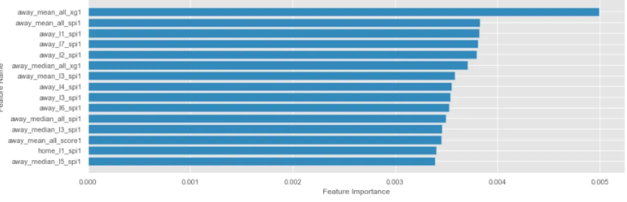
In order to select in the nodes the feature on which the node split will occur, tree-based al-gorithms need to calculate the feature importance. The feature importance calculation (Kuhn and Johnson,2013), visible in figure3.4, is based on how much the impurity is reduced across all trees in the forest when using a feature. This feature importance can be used as a selection technique for the models.
Figure 3.4: A visualization of an example of the feature importance in the random forest.
3.4
Machine Learning
The best simple definition of machine learning came in 1959 by Arthur Samuel. He described machine learning as “a field of study that gives computers the ability to learn without being ex-plicitly programmed”. Even though the exact quote exists in neither theSamuel(2000) paper nor the revised versionSamuel(1967), this is still the basis for many of the definitions of machine learning.
Machine learning is an auxiliary tool in the data mining context that allows for the creation of models using data. It gives us the possibility of creating models based on experience and observation, being able to create an inference mechanism that will then allow for generalization through induction. Its goal is to create a function y = f(x) that when given an instance x, makes a prediction y. The way that the function f(x) is inferred depends on the algorithm used.
In this chapter, we start by addressing the tasks that can be achieved using machine learning in the context of data mining. We then talk about the machine learning algorithms, focusing on the base learners that have the ability to predict probabilities. For last we do a brief overview of the evaluation metrics that can be used in the context of sports predictions.
14 Data mining concepts and techniques
3.4.1 Data mining tasks
The two high-level primary goals of data mining are prediction and description. Prediction in-volves predicting unknown values, and description focus on finding human interpretable patterns in data. These goals can be achieved using several methods (Fayyad et al.,1996):
• Classification
– Focus on learning a function that classifies a data instance into one of several prede-fined classes.
• Regression
– Focus on learning a function that maps a data instance to a real-valued prediction variable.
• Clustering
– Is a descriptive task where one seeks to identify a finite set of categories or clusters to describe the data.
• Summarization
– Consists of finding a model that describes significant dependencies between variables. • Change and deviation detection (also known as outlier/anomaly detection)
– Focus on discovering the most significant changes in the data from previously mea-sured or normative values.
3.4.2 Classification
Classification models (Kuhn and Johnson,2013) usually generate two types of predictions. Like regression models, classification models produce a continuous valued prediction, confidence level, which is usually in the form of a probability (i.e., the predicted values of class membership for any individual sample are between 0 and 1 and sum to 1). In addition to a continuous prediction, classification models generate a predicted class, which comes in the form of a discrete category.
If the models are well calibrated the resulting confidence levels from the models can be used as the predicted probabilities.
3.5 Algorithms 15
3.5
Algorithms
In this section we describe the algorithms used. These were the chosen algorithms because they showed good performance in previous academic work, unlike others like naive Bayes.
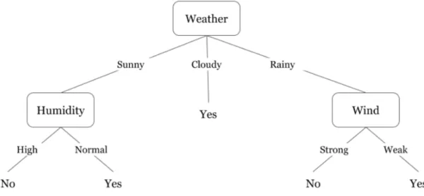
3.5.1 Decision trees
A decision tree (Kuhn and Johnson, 2013) falls within the category of tree-based models and consists of nested if-then statements, separating the data according to defined criteria. They can be highly interpretable, can handle many types of variables and missing data. However, they are unstable and may not produce optimal predictive performance.
Each node of the tree has a test that is made over a selected attribute and then divides into more nodes in a recursive process until the stopping criterion is met. In order to define the attribute used in order to split the node measures, such as the Gini index and cross entropy, can be used. Depending on the decision tree implementation many hyperparameters can be used. The most important is perhaps the maximum depth of the tree that when lowered allows for an increase in generalization power and thus reducing overfitting. In trade, the model complexity is reduced. A decision tree example can be seen in figure3.5.
Figure 3.5: A example decision tree classifying if a person should or not play badminton. SourceGupta(2019)
16 Data mining concepts and techniques
3.5.2 k-nearest neighbor
The k-Nearest neighbor is a distance-based algorithm: the predicted value for a new instance is calculated based on the k closest instances available in the data. That is, the algorithm searches for instances similar to the one that is trying to predict and uses the past results in order to make a new prediction.
The parameters that we need to set is how many neighbors we use (k) and how is the distance between two instances calculated. The distance can be calculated using Euclidean or Minkowski distance metrics. One factor (Kuhn and Johnson,2013) to take into account when using the k-NN is that the distance value between samples will be biased towards features with larger scales. This means that centering and normalizing or scaling the predictors will influence the performance of the algorithm.
The optimal k parameter is influenced by how many instances of data we have to train our model. A low ratio k/number of instances will lead to high difficulty in generalization since the influence of each of the instances is bigger and it leads to highly localized fitting. A high ratio will lead to instances that are not relevant to the prediction to be used and badly influence the results. The effect of the k value can be seen in figure3.6.
The addition of more data increases the efficiency of the algorithm due to the reduction of the k/number of instances ratio, however, this ratio needs to be tracked in problems where the amount of instances varies over time in order to readjust the model according to its needs.
Figure 3.6: A example of a k-nearest neighbor classification. It is visible the dependence of the prediction on the k value, since the prediction from k=1 is different from k=3.
3.5 Algorithms 17
3.5.3 Neural networks
Neural networks are aggregations of units called perceptron. A perceptron (Kuhn and Johnson,
2013) is a unit that calculates the linear combination of its inputs and then passes the result through an activation function. This can be seen in equation3.1, where y represents the predicted value and d the total number of inputs. The architecture of a perceptron can be seen in figure3.7.
Figure 3.7: Basic architecture of the perceptron. SourceAggarwal(2018) y= activation f unction( d
∑
j=1 wjxj) (3.1)The perceptron is able to produce classification models with great performance when data is linearly separable. However, many real problems do not have the luxury of being linearly separable. In order to be able to deal with non-linear problems, the perceptron needs to be able to approximate more complex functions. On its own, the perceptron does not have this ability.
To have this ability a network of perceptrons needs to be built. By aggregating perceptrons in a sequential network, the model is now able to approximate nonlinear functions. The shape of the network will limit the complexity of functions that can be approximated. In figure3.8we can see an example of a neural network.
The process throughout which the neural networks are usually trained is called back propaga-tion (Aggarwal,2018). It contains two main phases referred to as forward and backward phases. In the forward phase, the output values are calculated and compared to the actual value and then the gradient of the loss function is calculated according to the results. After that, in the back-ward phase, the gradients are used to update the weights. This phase is called the backback-ward phase because the gradients are learned from the output node to the input nodes.
While the ability of neural networks to be able to learn deep patterns in data may look like a positive point towards neural networks, sometimes this power can result in bad generalization results. To solve this problem several approaches can be used.
18 Data mining concepts and techniques
Figure 3.8: A visualization of a neural network with 28 inputs, 1 hidden layer of 15 nodes and 3 outputs.
The first approach is to introduce some form of regularization in the neural network. The reason for the lack of generalization ability comes from a large number of parameters, therefore, limiting the impact of these parameters will result in models with better generalization. One way to induce regularization is to use early stopping. When using early stopping the model will stop its training when the loss function fails to make sizable improvements over a certain period of time. This allows the patterns found in training to not become too deep, which is a source of generalization problems.
Another approach would be to use the dropout method (Aggarwal, 2018). In the dropout method, the network in each iteration of training selects a predefined set of nodes that will be trained during the iteration. This will incorporate regularization into the learning procedure. By dropping input and hidden units from the network, the dropout incorporates noise into the learning process, not allowing the model to learn deeper patterns.
Alongside with regularization techniques, a solution to the generalization problem is ensem-bling, and will be approached in the next chapter.
3.6 Evaluation metrics 19
3.6
Evaluation metrics
Every problem needs its own way of evaluating the obtained results. In the case of sports betting, the metrics that we are mostly interested in are related to measuring the efficiency of the bets that we make.
3.6.1 Accuracy
The accuracy (equation3.2) is a standard metric in classification problems.
accuracy= correct predictions
number o f predictions (3.2)
3.6.2 Profit (Rentability)
This evaluation metric is straight forward: we allow the model to make a one unit bet, and then, according to the outcome, add the profit/loss of the bet to our metric. Rentability is defined in equation3.3.
rentability=
∑
correct predictions
(odd− 1) − number o f incorrect predictions (3.3)
It gives us a broad perspective of how the models are performing. While the following metrics will give a result that is harder to interpret due to being influenced by more factors, this metric will give us the results that are more instinctively interpreted.
3.6.3 Return on investment (ROI)
The ROI metric, defined in equation3.4, is the ratio of profit to the total amount of money invested on the bets.
ROI= pro f it
investment (3.4)
This metric differs from the profit because it incorporates the amount of money invested. If we do unit bets it will allow us to differentiate between models with the same profit but make more or fewer bets. It is also easier to interpret from the business point of view: we know that if we bet 100 units in the model predictions we are expecting to win 100 * ROI units from those bets.
20 Data mining concepts and techniques
3.6.4 Difference between real profit and expected profit
Whenever we make a value bet we can calculate the amount that we are expecting to win in the long term by doing that bet. For example, if we bet in a 2.05 odd that should be a 2.00 odd we can expect to win 2.5 cents from that bet.
By comparing the profit that we are expected to obtain with the profit that actually has been made we can check if we are making a profit because the probabilities are correctly predicted or because we are simply getting lucky.
3.6.5 Ranked probability score
The ranked probability score (Weigel et al., 2006) is one where we can compare the calculated probabilities with the actual probabilities of the event happening.
The ranked probability score is defined in equation3.5, where M is the number of forecasts, γ the predicted probability and the Y the observed probability.
RPS=
M
∑
i=1
Chapter 4
Ensemble learning
There are several ways with which we can improve the performance of machine learning models. We are taking a look at the most common approach, ensemble learning.
In this chapter, we first take a look at and formulate the problem that we are trying to solve with ensemble learning. Then a quick example based on data from the our data set illustrates and confirms the formulation of the problem. After that, ensemble learning is defined and ensemble algorithms are presented for general use, for decision trees and for neural networks.
4.1
The generalization problem
With so much ability from the algorithms to learn the complex functions in many domains there comes the problem of overfitting the data whenever we are not careful enough with the design of the learning process. Overfitting (Aggarwal,2018) means that the algorithms provide excellent predictions on the training data, but performs badly when tested in previously unseen instances. In an extreme form of overfitting, it can be described as memorization of patterns in the data. Simply put, overfitted models do not generalize well to instances with which the models were not trained. This is especially evident in neural networks because of them being able to adapt to the training data.
The ability of a learner to provide useful predictions for instances it has never seen before is referred to as generalization (Aggarwal,2018).
4.2
Bias and Variance
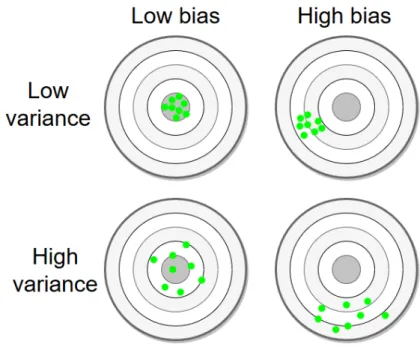
The generalization problem can be quantified by measures of the bias and variance errors. In figure
4.1we can visualize the effects on predictions.
4.2.1 Bias
Bias is related to the error caused by simplifying assumptions in the model that causes constant errors across different choices of training data. That is, if a model has high bias error it means that
22 Ensemble learning
Figure 4.1: Representation of the bias-variance problem as an analogy to the precision-accuracy. SourceFrank(2017)
it only recognized simple patterns in data and is a low complexity model, which causes the model to only make vague predictions. As stated byAggarwal(2018), this error cannot be removed even with an infinite source of data.
The bias error calculation for an instance is represented in equation4.1, where M is the number of predictions made, γ is the predicted value and y is the real value.
bias2= 1 M M
∑
i yi− γi (4.1) 4.2.2 VarianceVariance is the variability of model prediction for a given instance. A high variance means that a model learns deep patterns in the training data, creating high complexity models, that do not generalize well into the testing data. Slight changes in the training data induce big changes in the predictions. This error can be reduced by using bigger amounts of data.
An estimate of variance can be made by calculating the standard deviation of the predictions for each instance, as can be seen in equation4.2.
estimated variance= 1 M M
∑
i stdev(γi) (4.2)4.3 Scenario: Decision trees parameter optimization 23
4.2.3 Bias-Variance trade-off
Simple models result in a high bias and low variance, complex models in low bias and high vari-ance. The bias-variance trade-off allows us to find an intermediate point that allows us to minimize the sum of the bias and variance error.
Figure 4.2: Representation of how bias, variance and overall error moves according to the model complexity.
SourceAggarwal(2018)
As seen in figure4.2, there is an optimal model complexity that allows us to reduce the overall error, finding a compromise between the bias and variance error.
4.3
Scenario: Decision trees parameter optimization
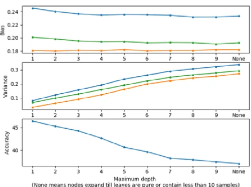
One of the ways to observe how bias and variance moves is to observe the predictions of a sim-ple model (decision tree), and compare how the bias and variance errors behave when we shift parameters.
This experiment consists of testing a simple decision tree regressor with default parameters, except the maximum depth. As stated in section3.5.1, the maximum depth is one of the parameters that we can use to tune the model complexity. The higher the maximum depth, the higher the model complexity.
The test was executed by training 50 different models each with a different data set generated by randomly selecting 50% of the instances in data. The used features are the goals scored and conceded in the last 7 games by the teams in the game we are trying to predict.
In figure4.3, we can confirm what was stated before: more complexity (models with higher maximum depth) leads to higher variance and lower bias.
24 Ensemble learning
Figure 4.3: Movement of the Bias-Variance trade-off according to the model complexity.
In a problem of this complexity, slight improvements on the bias error lead to heavy penaliza-tion in terms of variance error, with the variance error being dominant over the bias error. This can be verified in the accuracy of the models. Even though the bias error is being reduced the accuracy metric is unable to improve.
The result of this dominance of the variance error leads to the less complex models being able to predict with better accuracy. Isolating the maximum depth parameter allows us to observe that the optimal complexity of the decision tree model is with very low maximum depth.
4.4
Regularization
The reason for overfitting is that the model captures the noise in the train data. One of the ways to reduce overfitting is regularization. Regularization (Aggarwal,2018) is a form of penalizing the models for chasing complex models. This penalization is usually added in the loss function. It can be used in several machine learning algorithms.
Regularization parameters enable the model to be tuned to the optimal complexity of the mod-els by manipulating its complexity.
4.5 Ensemble 25
4.5
Ensemble
Another way of reducing the error of a classifier (Aggarwal,2018) is to find a way to reduce either the bias or the variance without affecting the other component.
The most used technique in order to reduce bias and variance is ensemble learning. Ensemble methods aggregate multiple models to obtain better performance than what could be obtained from any of the constituent models alone.
Ensemble learning has, depending on the algorithm used, several advantages: from reducing the bias and variance to the ability to be able to improve weak learners. However, it comes with the cost of several impacts on computational performance, due to the need for multiple models to be trained.
4.5.1 Bagging and Subsampling
The most used ensemble technique is bagging (Aggarwal,2018), also known as bootstrap aggre-gating, mainly due to its simplicity. The basic idea is to generate new training data sets from the single instance of the base data by sampling, which can be performed with or without replacement. An example can be seen in figure4.4.
Figure 4.4: Production of subsamples in bagging. Source:Shubham(2018)
Simply put, subsets of data are generated from the data set that contains a percentage of the instances. This creates variability which is the most important factor in the success of ensembles. Then, a predefined amount of models is trained on those data sets and predictions are made. The final prediction of the ensemble is a function of all the probabilities, usually average, possibly weighted, median values or voting.
26 Ensemble learning
Bagging and subsampling techniques are primarily directed towards reducing variance, how-ever, bias can also be slightly reduced.
4.5.2 Boosting
A boosting algorithm is an algorithm in which the primary goal is to reduce bias.
The most well known boosting algorithm is the AdaBoost (Freund and Schapire,1997). The name comes from "adaptative boosting" since it boosts a weak learner based on adjusting to the errors in its predictions.
The AdaBoost consists in iteratively improving a weak learner by changing the weights of data instances according to its predictions so that instances that are wrongly predicted have a bigger weight than correctly predicted instances, forcing the models to learn them.
The final prediction of a boosting model is a weighted average of the models from each itera-tion. The weight of each model usually decreases over the iterations.
This technique might also allow for a decrease in variance, when comparing with a single estimate. It also is able to substantially reduce bias error. The price to pay for that is that this kind of ensembles is that not only it does not help reducing overfitting but it also faces the problem of increasing overfitting, and that is a factor to take into account when choosing the ensemble to use.
4.6 Ensembling decision trees 27
4.6
Ensembling decision trees
4.6.1 Bagging and AdaBoostSince decision trees are usually unstable learners and have a high variability, they are able to make sizable improvements when ensembled. This is the case for both bagging and AdaBoost techniques. They are able to improve the results of the models in both bias and variance.
Even though both approaches work well, there are two algorithms that work with decision trees that are able to generate similar or better results.
4.6.2 Random forest
As defined byHo (1995), "the essence of the method (random forest) is to build multiple trees in randomly selected subspaces of the feature space". According to the author and proven by several experiences, when the trees are generated from different feature subspaces they tend to complement each other’s predictions, in a way that improves the classification accuracy, even when compared with bagging. The process of randomly selecting features for the model is called random subspace sampling.
The main difference from bagging is that not only are the instances subsampled, but also the features. This leads to increased variability from the trees that improves the ensemble model performance.
4.6.3 Gradient boosting
While in the AdaBoost algorithm the adaptation comes from giving more weight to the instances that are wrongly predicted, in the gradient boosting (Breiman,1997) the instances to which more weight is given is identified by gradients. The gradient boosting technique (Kuhn and Johnson,
2013) works on a defined loss function, and seeks to find an additive models that minimizes this loss function.
The gradient boosting technique does not work exclusive on decision trees like the random forest.
4.6.3.1 XGBoost
An improved version of the gradient boosting technique was later developed, the XGBoost. The most important advantages that the XGBoost holds over the gradient boosting (Chen and Guestrin,
28 Ensemble learning
4.7
Ensembling neural networks
In neural networks, ensemble methods are usually focused on variance reduction. This is because (Aggarwal,2018) neural networks are valued for their ability to build arbitrarily complex models, in which the bias is relatively low. This means that neural networks are able to generate high complexity models which leads to higher variance, manifested as overfitting. Therefore, when using neural networks we seek variance reduction in order to have better generalization prowess.
4.7.1 Bagging and boosting
While the bagging approach yields the expected results, high variance reduction and slight bias reduction, the boosting techniques fail to do so. Neural networks are already very strong learners and boosting techniques work better with weak learners in order to improve the models.
4.7.2 Negative correlation learning
Since ensemble models benefit from diversity between the base learners, it is useful to increase this diversity. In negative correlation learning (Liu and Yao,1999), the approach is to train individual networks in an ensemble and combining them in the same process. All the neural networks in the ensemble are trained simultaneously and interactively through a correlation penalty term in their error function.
The difference from regular neural network training is in the loss function. Subtracted to the regular loss function, that is a function of the predicted value and the real value, is a percentage of the loss function calculated between the value predicted by the model and the ensemble predicted value. This can be seen in equation4.3, where γ is a neural network prediction, ε the ensemble prediction and y is the real value. This incentives models to go in a different direction from the average value of the ensemble, creating diversity in the model’s opinions and improving the model classification performance.
Chapter 5
Data mining in the sports context
In this chapter, we take a look at the previous work done in the area of sports predictions. The search method was using Science Direct search engine to find the most relevant papers in the area, with a focus on the most recent work.
Academia has embraced the problem of predicting football matches very heavily. Some of the most notable work was done byConstantinou et al.(2012) with the usage of Bayesian networks in order to create an agent to predict probabilities in the English Premier League 2010/11 season, managing to obtain profit even though the test sample was very small. This model was then improved (Constantinou et al., 2013), reaching the conclusion that a less complex model can perform better, which suggests that selecting the right data is more important than just having a lot of data.
Bayesian networks seem to be the go-to prediction method in academia. Joseph et al.(2006) evaluated the predictions made by an expert-made Bayesian network for the London team Totten-ham Hotspurs in the seasons of 1995/96 and 1996/97 and compared them with some of the state of the art machine learning prediction algorithms, like MC4 decision trees, naive Bayes, data-driven Bayesian and a K-nearest neighbour learner. The conclusion was that expert-based Bayesian net-works were way more reliable at predicting the outcome of games, although this was probably due to the type of data available not fitting the algorithms used, with some of the attributes being the boolean variables to check if the most important Tottenham players were playing in the game. There was also a problem in the data dimensionality that leads to the results being biased towards the Bayesian network.
Owramipur et al.(2013) confirmed once again that Bayesian networks perform very well under the right conditions, as they were able to predict Barcelona games in the Spanish La Liga with 92% accuracy, which is not the best metric to evaluate the models for a team that is favourite to win every game, but shows its efficiency.
Rotshtein et al.(2005) used fuzzy based models with genetic and neural tuning to predict the results of games for the football championship of Finland, which achieved interesting results as it was done in data set with a low number of attributes. It predicted the spread (the difference between two teams score in a game) based only on previous results.
30 Data mining in the sports context
There is some relevant work done in predictions using neural networks.Mccabe and Trevathan
(2008) compares the behaviour of artificial neural networks predicting football and rugby matches, reaching the conclusion that the predictions are better in sports with a lesser percentage of draws. The better accuracy in sports with a lesser percentage of draws comes from the fact that the draw is never the most expected result. This means that, in general, classification models do not predict draws since the probability of a draw is always lower than any of the probabilities of the teams to win the game.
Neural networks are also useful in predicting the sports betting exchanges movements.Dzalbs and Kalganova(2018) used artificial neural networks and cartesian genetic programming in order to test automated betting strategies in a betting exchange using the Betfair API.
Another relevant work was done byHvattum and Arntzen(2010) by adapting the ELO rating system in order to make football predictions. The ELO rating system was developed byElo(1978) to quantify the strength of chess players. There are similar ELO inspired rating systems but no relevant studies were found on them. Rating systems might be useful because they might allow us to generate important features for models.
A full data mining methodology was done byBaboota and Kaur(2019). The unanimously considered a crucial aspect in the data mining process is the feature engineering which is entirely dependent on the data that is available. The machine learning algorithms used were naive Bayes, support vector machines, random forest and gradient boosting. The ensemble algorithms, random forest and gradient boosting, are the algorithms that better perform, suggesting that ensemble algorithms are the go-to techniques in order to have the best predictions.
It is suggested the usage of a performance metric proposed by Epstein (1969), the ranked probability score, that measure how well forecasts are expressed as probabilities according to the observed outcome. Another metric that is relevant is the “losses per unit bet” (Buhagiar et al.,
2018), where the performance of an algorithm is set by the results of the bets that the algorithm makes.
A summary of the literature review from the point of view of prediction methods can be seen in table5.1.
On the topic of sports betting, one of the most studied phenoms studied in academia was the favourite-longshot bias – the odds that the bookmakers show are better at predicting the probabil-ities for the favourite to win than predicting the lower probabilprobabil-ities.Buhagiar et al.(2018) studies and confirms the existence of the favorite-longshot bias. The reason given is that the longshots are riskier for bookmakers if incorrectly priced, leading to a bigger tax on these odds. While the favourite-longshot bias might not be enough in order to make a profit it might lead to better results when exploited.
Data mining in the sports context 31
Table 5.1: A brief summary of the literature review.
Reference Method Data set Seasons Best algorithm Accuracy
Constantinou et al.(2012) BN English PL 2010/2011 -
-Constantinou et al.(2013) BN English PL 1993 to 2010 -
-Joseph et al.(2006) BN vs Machine learning Tottenham games 1995 to 1997 K-NN 50,58%
Owramipur et al.(2013) BN Barcelona games 2008/2009 - 92%
Rotshtein et al.(2005) Fuzzy model Finnish PL 1994 to 2001 -
-Mccabe and Trevathan(2008) NN English PL 2002 to 2006 - 54,60%
Dzalbs and Kalganova(2018) NN BetFair odds 1 Jan to 17 May 2016 -
-Hvattum and Arntzen(2010) ELO-based 4 English divisions 1993 to 2008 -
Chapter 6
The approach to the problem and
results
As stated before, the used methodology was CRISP-DM. This chapter summarizes the methodol-ogy, results and conclusions of the developed experiences. The structure of this chapter follows the CRISP-DM methodology.
6.1
Business understanding
6.1.1 Determine the business objectivesFollowing the CRISP-DM methodology, the first step is the business understanding phase. In this phase, after research on the topic was made, the following business objectives were set:
• Calculate probabilities of football games.
• Verify calculated probabilities on different betting strategies. • Extract value from the predictions.
Alongside these objectives, the business success criteria were also defined: • Obtain a positive ROI.
34 The approach to the problem and results
6.1.2 Determine the data mining goals
From the business objectives derived the data mining goals and success criteria. • Data mining goal
– Obtain models that calculate probabilities of football games winners (1x2), maximiz-ing its accuracy in order to calibrate its probabilities.
• Data mining success criteria
– Models have a positive ROI from the point of view of the bettor.
6.1.3 Assess the situation
On the development of the project the following tools were used: • Python programing language
– pandas – sklearn
– keras (tensorflow interface) – matplotlib and networkx – beautifulsoup
It was also assessed which data was freely available for use. The free data sets that were available and relevant in this context were:
• football-data.co.uk (Football-Data.co.uk) – general statistics and odds from matches • fivethirtyeight.com (FiveThirtyEight) – complex football statistics such as expected goals
6.1 Business understanding 35
6.1.4 Evaluation metrics
In order to be able to evaluate the models, key metrics were defined. Some of these metrics are general and found in several other machine learning problems, others are business specific metrics to evaluate the betting performance of the models.
• General
– Accuracy (defined in3.6.1) – Percentage of correct predictions.
– Bias (defined in 4.2.1) – Difference between the mean of the model predictions and the correct value.
– Estimated variance (defined in4.2.2) – Variability of the model prediction for a given instance.
• Specific
– Profit (defined in3.6.2) – Rentability of the models.
– Return on Investment (ROI) (defined in3.6.3) – Profit/Investment.
All of these metrics depend on how we interpret the results from the models. In this case, two different strategies are used:
• Strategy 1
– Bet on the algorithm’s favorite.
– This strategy is more focused on the classification part of the problem. • Strategy 2
– Bet when the odd of the bookmaker is bigger than the odd calculated by the algorithm. – This strategy is more focused on the regression part of the problem.
The specific metrics also depend on how we manage our budget. Two different approaches are evaluated:
• Unit betting
– Each bet is 1 unit. • Bank Percentage betting