Rafael de Braga Castilho
Essays in Industrial Organization
Rio de Janeiro 2017
Essays in Industrial Organization
Tese para obtenção do grau de doutor apresentada à Escola de Pós-Grauação em Economia
Área de concentração: Organização Indus-trial
Orientador: Luis Henrique Bertolino Braido
Rio de Janeiro 2017
Castilho, Rafael de Braga
Essays in industrial organization / Rafael de Braga Castilho. – 2017. 49 f.
Tese (doutorado) - Fundação Getulio Vargas, Escola de Pós-Graduação em Economia.
Orientador: Luis Henrique Bertolino Braido. Inclui bibliografia.
1. Organização industrial. 2. Preços – Discriminação. 3. Fundo mútuo de renda fixa. 4. Comportamento do consumidor. I. Braido, Luis H. B. II. Fundação Getulio Vargas. Escola de Pós- Graduação em Economia. III. Título.
Agradeço ao meu orientador Luis Braido pela paciência e tempo gasto comigo, à Helena Perrone pela orientação durante a minha estada em Barcelona e participação na banca, ao Andre Trindade pelo auxílio no segundo artigo e participação na banca. Também agradeço aos demais membros da banca, aos funcionários (em especial Andrea e Aline), o auxílio financeiro da CAPES e do CNPq. Agradeço aos meus pais Leila e Pedro pelo apoio durante estes 6 anos de EPGE (além dos 24 antes), à Nathália por me acompanhar nos momentos bons e nas angústias nestes últimos anos e, last but not least, agradeço à 1025, Iguana, Magal’s, Voluntários, Bambina, dentre outros, pelas salidas de copas.
O que é bonito?
É o que persegue o infinito; Mas eu não sou
Eu não sou, não...
Eu gosto é do inacabado,
O imperfeito, o estragado, o que dançou O que dançou...
Eu quero mais erosão Menos granito.
Namorar o zero e o não, Escrever tudo o que desprezo E desprezar tudo o que acredito. Eu não quero a gravação, não, Eu quero o grito.
Que a gente vai, a gente vai E fica a obra,
Mas eu persigo o que falta Não o que sobra.
Eu quero tudo que dá e passa. Quero tudo que se despe, Se despede, e despedaça. O que é bonito...
Esta tese é composta de três artigos, cada um correspondendo a um capítulo. No primeiro capítulo, eu analiso em que medida a correlação negativa entre a aplicação mínima inicial e a taxa de administração dos fundos de investimentos podem ser explicadas pelos custos ou se refletem a tentativa dos bancos de praticarem discriminação de preços de segundo grau. Usando um modelo estrutural eu recupero o custo marginal dos fundos e calculo quanto da variação da taxa é devido a diferenças de custo. No segundo capítulo eu apresento um modelo de comportamento dos consumidores e da firma com custos de troca para investigar como os preços variam com diferentes níveis de custos de troca. No terceiro capítulo eu apresento um modelo de comportamento da firma em um mercado oligopolístico com tarifas em duas partes e agentes heterogêneos. Um procedimento de estimatimação é apresentado e os dados sintéticos gerados são usados para recuperar os parâmetros estruturais.
This thesis is composed of three articles, each one corresponding to a chapter. In the first chapter I analyze the extent to which the negative correlation between funds minimum initial application and fees can be explained by costs or rather reflect banks attempt to practice second-degree price discrimination. Using a structural model of consumer and pricing behavior I recover funds marginal cost and therefore compute how much of the fee variation are due to cost differences. In the second chapter I present a model of consumer and pricing behavior with switching costs to investigate how prices vary with different switching costs levels. In the third chapter I present a model of firm behavior in a oligopolistic market with two-part tariffs and heterogeneous agents. An estimation procedure is presented and a synthetic generated data is then used to recover the structural parameters.
1.1 Histogram Administration Fee . . . 4
1.2 Histogram Minimum Initial Application . . . 4
1.3 Adm Fee and Min Init Appl . . . 5
1.4 Market Share of the largest 6 banks. . . 6
1.5 Total Net Asset . . . 6
1.6 Number of Funds . . . 7
1.7 Minimum, maximum, mean and counterfactual administration fee for each bank . 16 1.8 Minimum, Maximum and Mean of the Minimum Initial Application for each bank 17 2.1 Prices with different switching cost levels . . . 30
2.2 Market shares with different switching cost levels . . . 30
2.3 Profits with different switching cost levels . . . 31
1.1 Descriptive Statistics . . . 7
1.2 Demand parameters estimate . . . 13
1.3 Supply parameter estimates . . . 14
1.4 Counterfactual Results . . . 17
2.1 Switching costs . . . 28
2.2 Results. . . 29
2.3 Results. . . 36
1 Minimum Initial Application and Price Discrimination in the Fund Market 1
1.1 Introduction . . . 1
1.2 Brazilian Fixed Income Fund Market and Price Discrimination . . . 3
1.3 Data . . . 5
1.4 Empirical Framework and Estimation. . . 8
1.4.1 Demand . . . 8
1.4.2 Supply . . . 9
1.4.3 Estimation . . . 10
1.4.4 Endogeneity. . . 11
1.5 Results. . . 12
1.6 Counterfactual and Welfare Analysis . . . 15
1.7 Conclusion. . . 19
1.8 Appendix: Computational Details. . . 19
2 Can Switching Costs Reduce Prices? 21 2.1 Introduction . . . 21 2.2 Model . . . 22 2.2.1 Consumer Problem . . . 23 2.2.2 Aggregate Demand . . . 25 2.2.3 Supply . . . 26 2.2.4 Equilibrium . . . 26 2.3 Simplified Model . . . 27 2.4 Model Predictions . . . 28 2.5 Estimation Algorithm . . . 31 2.6 Conclusion. . . 33 2.7 Appendix . . . 33
2.7.1 Synthetic Data-Generating Process . . . 33
2.7.2 Algorithm . . . 34
2.7.3 Estimation Steps . . . 34
2.7.4 Grid and Transition Matrix . . . 35
2.7.5 Numerical Example . . . 36
3 Estimating an oligopoly model with differentiated goods and two-part tariffs 37 3.1 Introduction . . . 37 3.2 Model . . . 38 3.2.1 Market Share . . . 40 3.2.2 Supply . . . 40 3.3 Estimation . . . 43 3.4 Numerical Example. . . 44 3.5 Conclusion. . . 46 3.6 Appendix . . . 46
Minimum Initial Application and Price
Discrimination in the Fund Market
1.1 Introduction
Price dispersion is present in several markets, including the investment fund market. Funds could hardly be considered homogeneous products, since its characteristics like return, risk and portfolio composition vary. Although the fee variation could solely reflect cost differences, it could also be due to markup differences.
In this paper I analyze the roles of cost differences and second-degree price discrimination in explaining the observed fee dispersion in the fund industry. To do this I use a model that allows to recover the marginal cost and therefore decompose the fee into the marginal cost and a markup term. A fee decrease mostly due to markup variation as minimum initial application increases suggests the presence of price discrimination.
With this purpose I estimate a structural model of consumer and pricing behavior that allows for consumer and fund heterogeneity. Consumers value funds characteristics and choose the fund that maximizes utility. Consumers are heterogeneous in their valuation of fund characteristics and therefore choose different funds. Banks are profit maximizing multi-product firms that compete in prices. The results can give a better idea of how the competition plays in this relevant market and thus suggest some guidelines on policy.
The existence of fee dispersion in the fund industry has already been studied by other papers, but never - at least to my knowledge - as reflecting bank attempt to price discriminate. Hortaçsu and Syverson (2004) estimate a structural model with consumer heterogeneity in search costs
and funds vertically differentiated. They estimate nonparametrically a c.d.f. of the search cost distribution which rationalizes the observed market shares. While Iannotta and Navone
(2012) controls for funds observable sources of heterogeneity and attribute to search costs the fee dispersion not explained.
Some papers study the price discrimination empirically. Cohen(2008) investigate the extent to which quantity discounts for paper towels are consistent with second degree price discrimi-nation. The presence of nonlinear pricing in the specialty coffee market is studied in McManus
(2007). Leslie (2004) presents a structural model with both second and third degree price dis-crimination using data for a Broadway play. He found an increase of 5% in firm profit relative to uniform pricing and no difference in consumer surplus. Busse and Rysman(2005) studied the market for advertising in Yellow Pages diretories and noticed that purchasers of the largest ads pay less per ad size relative to those of small ads, even though this being more competitive.
Data were provided by Brazilian Financial and Capital Markets Association (Anbima) and consist of monthly information for Brazilian funds. Anbima classifies funds in mutually exclusive categories such as short term, multimarket, pension, DI referenced, fixed income and shares, which allows for different portfolio composition. Among these categories, I only consider fixed income, which is the largest category, including over 1000 funds and 25% of the 2 trillion Brazilian Reais (BRL) net asset.
With the purpose of access how fees, minimum initial applications and consumer welfare would change in a scenario where banks could not charge multiple fees nor minimum initial application, I use the model estimates to simulate two counterfactual scenarios. In the first, each bank can charge a unique administration fee for its funds, given the minimum initial application observed in the data. In the second, given a minimum initial application, the bank chooses a unique administration fee.
Results indicate that an increase of 100 BRL in the minimum initial application decreases the marginal cost in 0.002408 BRL. Using the parameters estimates I recover the marginal costs and obtain the fund’s markups, which decreases with larger minimum initial applications and therefore suggest the presence of second-degree price discrimination.
For the counterfactuals the predicted administration fee decreases monotonically with the minimum initial application and to achieve the administration fees charged with the observed minimum initial application (first counterfactual), it would be necessary an initial application around 20000 BRL for all funds. The change in consumer surplus is negative in the first
coun-terfactual and is positive in the second councoun-terfactual only for initial applications above 30000 BRL.
The remainder of this paper is organized as follows. Section 1.2describes the Brazilian fund market. Section1.3presents the data used. Section3.2presents the model of consumer and firm behavior, the estimation procedure and discusses identification. Section 1.5 shows the results and discuss the possibility of price discrimination. Section2.4 presents the counterfactuals and the welfare analysis. Section3.5concludes. Appendix1.8presents the computational procedure in details.
1.2 Brazilian Fixed Income Fund Market and Price
Discrimina-tion
The CVM 409 instruction regulates fund market in Brazil,1 It provides a mutually exclusive
classification of funds in categories such as short term, multimarket, pension, DI referenced, fixed income, shares. Fixed income is the largest fund category regarding net asset and holds around 25% of the 2 trillion BRL existent in this market.
Funds also need to specify some of its characteristic. If it is open or closed, which investor segment it is interested and if it has performance, entry or exit fees.2
A fund is classified open if its shareholders can request withdrawal before the end of its term.3 Otherwise it is classified as closed and withdraws can only occur at the end of the term,
previously defined.
The administration fee is charged annually as a percentage of the amount invested. While the performance fee is calculated based on the return that exceeds a certain percentage of the benchmark. The performance fee is charged with a predefined periodicity.
Entry and exit fees are charged at the moment of application and withdraw, respectively. Figure1.1present the administration fee histogram.
1This can be found athttp://www.cvm.gov.br.
2Sitehttp://www.anbima.com.br/mostra.aspx/?op=z&id=112contains the characteristics and rules. 3Each fund has to specify maximum periods between the shareholder request, conversion and receipt of a withdrawn.
0 .2 .4 .6 .8 Density 0 2 4 6 8 10 Administration Fee
Histogram Administration Fee
Figure 1.1: Histogram Administration Fee
Generally, funds set minimum initial applications and therefore consumers can not invest any amount initially. Figure 1.2shows the minimum initial application histogram.
0 5.0e-05 1.0e-04 1.5e-04 2.0e-04 Density 0 50000 100000 150000 200000
Minimum Initial Application
Histogram Minimum Initial Application
Figure 1.2: Histogram Minimum Initial Application
Each point at Figure1.3is the administration fee and minimum initial application for a fund in a month. The correlation between these variables is -0.4382.
-5 0 5 10 Administration Fee 0 50000 100000 150000 200000
Minimum Initial Application Administration Fee Fitted values
Figure 1.3: Adm Fee and Min Init Appl
1.3 Data
I use two sources to construct the dataset. The information on funds was provided by the Brazilian Financial and Capital Markets Association (Anbima) and consists of monthly infor-mation on all existing funds in Brazil from January 2000 to June 2012. The data on consumer characteristics are from the National Household Sample Survey (PNAD).
Anbima classifies funds into categories whose last reclassification was in August 2006. To avoid consider funds that are now into another category the dataset used starts in 2007. Since funds start and end during this period, the dataset is an unbalanced panel.
In the considered period there was a total of 174 funds offered by 26 banks. Figure1.4shows the market share of the largest banks, which contain almost ninety percent of the total market share.
0 .1 .2 .3 .4 .5 .6 .7 .8 .9 1 Market Share 2007m1 2008m1 2009m1 2010m1 2011m1 2012m1 Date Itaú HSBC Caixa Bradesco
Banco do Brasil Santander
Figure 1.4: Market Share of the largest 6 banks
Since few funds have another fee then the administration fee, I will only consider those that has only the administration fee along being offered by the six largest banks.4 This leads to a
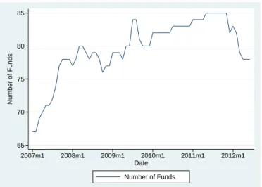
sample with 5255 observations and 104 funds. Figure1.5and Figure1.6present respectively the evolution of the net asset and number of funds.
5.000e+10 5.500e+10 6.000e+10 6.500e+10 Net Asset 2007m1 2008m1 2009m1 2010m1 2011m1 2012m1 Date Total Net Asset
Figure 1.5: Total Net Asset
65 70 75 80 85 Number of Funds 2007m1 2008m1 2009m1 2010m1 2011m1 2012m1 Date Number of Funds
Figure 1.6: Number of Funds
Table 1.1presents some descriptive statistics of the variables considered. The age of a fund (Age) is the number of months of existence divided by 12. Minimum initial application (Min Init Appl) and minimum additional application (Min Addit Appl) are in tens of thousands of BRL. Market share of the outside good (Mkt Share Out Good) is the market share of the funds not considered, ie, those with fees other than administration or that are not offered by the banks considered. Therefore the option to not consume one of the funds considered means its substitution to one from a non-considered bank or with fees other than the administration fee. I do not intend to explain the portfolio allocation between different kinds of investment and thus restrict the choices available to fixed income funds.
Table 1.1: Descriptive Statistics
Variable Mean Median Standard Deviation Minimum Maximum
Admin Fee 2,233 2 1,3147 0,4 11
Age 9,5944 10 5,6686 0 32,4167
Monthly Return 0,7077 0,7048 0,3935 -4,7534 17,3919
Min Init Appl 1,7695 0,5 2,7532 0 20
Min Addit Appl 0,0536 0,01 0,148 0 1
Number of Funds 78 78 4,2172 65 83
Mkt Share Out Good 14,29 15,19 4,67 7,08 26,12
Lastly, PNAD is a survey conducted by the Brazilian Institute of Geography and Statistics (IBGE) and I use the data on consumer income from 2007 to 2011. This data serves to generate
dispersion in consumers sensibility to funds characteristics, as will be explained in details next section.
1.4 Empirical Framework and Estimation
To access how much of the price variation is due to changes in the marginal cost, I estimate a structural model of consumer and pricing behavior that allows recovering the marginal cost for each fund. Consumers value funds characteristics and choose the one that maximize their utility, while banks are multi-product firms that compete in prices and maximize profits.
I also discuss the estimation procedure and how endogeneity emerges and is corrected in this framework.
1.4.1 Demand
The demand is similar to the random coefficients logit presented inBerry et al.(1995). Consumer 𝑖chooses fund 𝑗 (omitting the time subscript 𝑡 to simplify notation) and obtains utility
𝑢𝑖𝑗 = 𝑥𝑗𝛽𝑖− 𝛼𝑖𝑝𝑗 + 𝜉𝑗+ 𝜖𝑖𝑗 (1.1)
where 𝑥𝑗 is a k-dimensional vector of fund observed characteristics, 𝜉𝑗 is the unobserved (by the
econometrician) funds characteristics, which represents quantifiable characteristics that are not available in the data and unquantifiable characteristics like prestige and reputation Administra-tion fee is given by 𝑝𝑗 and 𝜖𝑖𝑗 is an idiosyncratic shock to consumer utility.5
The observed characteristics considered are the fund administration fee, minimum initial application, age and monthly return.
Parameters 𝛼𝑖 and 𝛽𝑖 capture the consumer 𝑖 taste for the price and observed characteristics.
These have the following functional form ⎛ ⎜ ⎝ 𝛼𝑖 𝛽𝑖 ⎞ ⎟ ⎠= ⎛ ⎜ ⎝ 𝛼 𝛽 ⎞ ⎟ ⎠+ Π𝑑𝑖+ Σ𝜈𝑖 (1.2)
where 𝑑𝑖 is a d-dimensional vector of individual demographic characteristics and 𝜈𝑖 is a
(k+1)-dimensional vector of individual shocks. The parameters 𝛼 and 𝛽 are consumers mean taste
5Where 𝜖 𝑖𝑗
𝑖𝑖𝑑
over the observed characteristics. While Π is a (k+1)×d matrix of parameters that captures the effects of demographics on consumer deviates from the mean taste and Σ is a diagonal matrix of parameters that captures the effects of individual shocks on tastes. Therefore with 𝑘 observed characteristics (other than price), there are 2(𝑘 + 1) + 𝑑(𝑘 + 1) parameters to be estimated
Hence the utility obtained from investing in a fund depends on its characteristics and con-sumer tastes. Furthermore, agents with different tastes may choose different funds.
The utility consumer 𝑖 receives from good 𝑗 can also be written as
𝑢𝑖𝑗 = 𝛿𝑗+ 𝜇𝑖𝑗 + 𝜖𝑖𝑗 (1.3)
where 𝛿𝑗 = 𝑥𝑗𝛽 − 𝛼𝑝𝑗+ 𝜖𝑖𝑗 is the mean utility of good 𝑗 and 𝜇𝑖𝑗 = [𝑝𝑗 𝑥′𝑗] · [Π𝑑𝑖+ Σ𝜈𝑖]is consumer
𝑖deviate from this mean.
Considering this is a discrete choice model, each consumer must choose one and only one fund. The outside good 𝑗 = 0 represents consumer option of not buying any of the 𝐽 funds and has normalized mean utility 𝛿0 = 0. This can be thought as the consumer ability to substitute
to other markets. Note that without the outside good, a homogeneous increase in the price of all funds does not change the market demand.
Fund 𝑗 market share is the integral over the set of consumer tastes that lead to its choice
𝑠𝑗(𝑝,𝑥,𝜉; 𝜃) =
∫︁
{𝑑𝑖,𝜈𝑖,𝜖𝑖|𝑢𝑖𝑗>𝑢𝑖𝑘 ,∀𝑘̸=𝑗}
𝑑𝐹𝑑(𝑑)𝑑𝐹𝜈(𝜈)𝑑𝐹𝜖(𝜖) (1.4)
where 𝜃 = (𝛼,𝛽,Π,Σ) and 𝐹𝑑, 𝐹𝜈 and 𝐹𝜖 are the CDF of consumer demographics, shocks and
idiosyncratic shocks respectively. Integrating in 𝜖, as shown inMcFadden(1974), gives 𝑠𝑗(𝑝,𝑥,𝜉; 𝜃) = ∫︁ 𝑑,𝜈 𝑒𝑥𝑗𝛽𝑖−𝛼𝑖𝑝𝑗+𝜉𝑗 1 +∑︀ 𝑘𝑒𝑥𝑘𝛽𝑖−𝛼𝑖𝑝𝑘+𝜉𝑘 𝑑𝐹𝑑(𝑑)𝑑𝐹𝜈(𝜈) (1.5) 1.4.2 Supply
F multi-product banks are offering each one some subset 𝒥𝑓 of the 𝐽 funds. Banks choose funds
administration fees in order to maximize profits considering other banks funds characteristics and administration fees. The profit function for bank 𝑓 is given by
Π𝑓 =
∑︁
𝑗∈𝒥𝑓
(𝑝𝑗− 𝑚𝑐𝑗)𝑀 𝑠𝑗(𝑝,𝑥,𝜉; 𝜃) (1.6)
where 𝑝𝑗 is the administration fee, 𝑚𝑐𝑗 the marginal cost and 𝑀 the market size. The marginal
cost has the following functional form
𝑚𝑐𝑗(𝑥𝑐𝑗,𝜔𝑗; 𝛾) = 𝑥𝑐𝑗𝛾 + 𝜔𝑗 (1.7)
where 𝑥𝑐
𝑗 and 𝜔𝑗 are the observed and unobserved cost characteristics respectively. The observed
characteristics that influence marginal cost are the minimum initial and additional application and the net asset. There are also dummies for each bank and a trend.
1.4.3 Estimation
I follow Berry et al. (1995) to estimate the demand parameters 𝛼, 𝛽, Π and Σ along with the supply parameter 𝛾. This consists in isolate the error terms 𝜉, 𝜔 and interact them with the proper set of instrumental variables to form the moment conditions and then use a GMM estimator.
Next I present the estimation procedure, while the computational details are in Appendix
1.8. For more details seeBerry et al.(1995) or Nevo(2000).
From demand subsection, the market share of fund 𝑗 is given by the integral in equation1.5. This integral does not have a closed form and therefore is integrated using simulation. With a guess of the parameters values Π, Σ, one vector of products mean utilities 𝛿 and 𝑛𝑠 pseudo random draws of consumer tastes, calculate
𝑠𝑗(𝛿,𝑝,𝑥; Π,Σ) = 1 𝑛𝑠 𝑛𝑠 ∑︁ 𝑖=1 𝑒𝛿𝑗+𝜇𝑖𝑗(Π,Σ) 1 +∑︀𝐽 𝑘=1𝑒𝛿𝑘+𝜇𝑖𝑘(Π,Σ) (1.8)
I iterate over the operator defined below to obtain the vector of mean values 𝛿 that equalizes the predicted and the observed market shares
where 𝑆 is the vector of observed market shares.6 The error term can be written as
𝜉𝑗 = 𝛿𝑗− 𝑥𝑗𝛽 + 𝛼𝑝𝑗 (1.10)
For the supply side, it is obtained the FOC of the profit function in equation1.6
𝑠𝑗(𝑝,𝑥,𝜉; 𝜃) + ∑︁ 𝑟∈𝒥𝑓 (𝑝𝑟− 𝑚𝑐𝑟) 𝜕𝑠𝑟(𝑝,𝑥,𝜉; 𝜃) 𝜕𝑝𝑗 = 0 ,∀𝑗 ∈ 𝒥 (1.11)
and in vector notation is
𝑠(𝑝,𝑥,𝜉; 𝜃) − ∆(𝑝,𝑥,𝜉; 𝜃)[𝑝 − 𝑚𝑐] = 0 (1.12)
with ∆𝑗𝑟(𝑝,𝑥,𝜉; 𝜃) = −
𝜕𝑠𝑟
𝜕𝑝𝑗 1𝑗𝑟, where 1𝑗𝑟 is an indicator function that assumes value 1 if 𝑗 and
𝑟 are sold by the same bank and 0 otherwise.
Replacing the marginal cost in the FOC and rearranging
𝜔 = 𝑝 − 𝑥𝑐𝛾 − ∆(𝑝,𝑥,𝜉; 𝜃)−1𝑠(𝑝,𝑥,𝜉; 𝜃) (1.13)
The identification condition also followsBerry et al.(1995) and entails that under appropriate instruments Z, at the true parameters values E(𝜉
𝜔|𝑍) = 0.
Therefore given the appropriate instruments I use a GMM procedure to estimate the param-eters, ie, search over the parameters 𝛼, 𝛽, Π and Σ that makes the sample moments as close as possible to zero. The computational details are provided in the Appendix1.8.
1.4.4 Endogeneity
The endogeneity appears since it is expected that some of the observable characteristics (𝑥,𝑝) are correlated with the unobservable 𝜉 as well as some elements of 𝑥𝑐 are correlated with 𝜔.
For demand I suppose that fund characteristics (other than administration fee) 𝑥 are exoge-nous to the unobserved product characteristics 𝜉. While for supply all cost characteristics 𝑥𝑐are
supposed to be exogenous. Therefore I am concerned about the correlation between price 𝑝 and unobservables 𝜉 and 𝜔.7
6InBerry et al.(1995) it is shown the existence and uniqueness of the 𝛿 vector and that the operador1.9is a contraction. Therefore any initial guess of 𝛿 will lead to the same fixed point.
As inBerry et al. (1995) I assume that supply and demand unobservables are mean indepen-dent of both observed product characteristics and cost shifters, i.e.
E(𝜉𝑗|𝑥, 𝑥𝑐) = E(𝜔𝑗|𝑥, 𝑥𝑐) = 0 , ∀𝑗
where 𝑥 = (𝑥1, . . . , 𝑥𝐽)and 𝑥𝑐= (𝑥𝑐1, . . . , 𝑥𝑐𝐽).
The instrument matrix for demand and cost shifters are 𝑧𝑑= (𝑧𝑑
1, . . . , 𝑧𝐽𝑑)′and 𝑧𝑐= (𝑧1𝑐, . . . , 𝑧𝐽𝑐)′,
respectively. Instruments for demand/cost for fund 𝑗 are a function of the exogenous observed demand/cost shifters
𝑧𝑗𝑑= 𝑧𝑑(𝑥1, . . . , 𝑥𝐽) and 𝑧𝑗𝑐= 𝑧𝑐(𝑥𝑐1, . . . , 𝑥𝑐𝐽)
with #(𝑧𝑑
𝑗) > #(𝑥𝑗) and #(𝑧𝑗𝑠) > #(𝑥𝑐𝑗) , ∀𝑗 to satisfy the necessary order condition for
identification.
Let 𝑧𝑗𝑘 be the 𝑘th exogenous characteristic of product 𝑗 and consider
𝑧𝑗𝑘 , ∑︁ 𝑟̸=𝑗,𝑟∈𝒥𝑓 𝑧𝑟𝑘 , ∑︁ 𝑟̸∈𝒥𝑓 𝑧𝑟𝑘
the first is the proper 𝑘th characteristic of product 𝑗, the second is the sum of this characteristic over the products produced by the same firm and third is the sum across other firms. Then, if there are 𝐾 − 1 exogenous observed characteristics for demand, there are 3(𝐾 − 1) instruments for the price. For supply it is used the cost shifters.
1.5 Results
Results from estimation of demand and supply parameters are shown in Table 1.2 and 1.3, repectively. First column of Table 1.2 presents the values of mean coefficients 𝛼 and 𝛽. Next columns display the coefficients that capture the heterogeneity in tastes, i.e., the shocks Σ , income and logarithm of income Π.
(2003), price coefficient is biased downward (in modulus) if higher prices are associated with desirable attributes, because the estimated price coefficient captures both price effect and desirable unobserved attributes effects. While opposite direction occurs if a price decrease is made jointly with an increase of advertising, for example. The increase in demand comes from both effects and price coefficient is biased upward (in modulus).
The mean coefficient on administration fee has the expected negative sign. Minimum initial application coefficient has a positive sign as well as age. Differently than expected, the mean effect of monthly return is negative.
The positive sign in the coefficients that captures the interaction between administration fee and income indicates that persons with more income are less price sensitive.
Table 1.2: Demand parameters estimate Demand Side Parameters
Variable Mean Shocks log(Income) Income
Constant -4.6270*** -0.0019 0.0465*** -0.0016
(0.0003) (0.0032) (0.0009) (0.0029)
Admin Fee -0.5443*** -0.0212*** 0.0002 0.0141***
(0.0003) (0.0028) (0.0009) (0.0016)
Min Init Appl 0.1126*** -0.0105*** 0.0099*** 0.0320***
(0.0002) (0.0027) (0.0006) (0.0012)
Age 0.1209*** 0.0012*** -0.0040*** -0.0008***
1.0e-03· (0.0627) (0.3556) (0.0726) (0.3377)
Monthly Return -0.0342*** 0.0403*** 0.0142*** -0.0913***
(0.0005) (0.0015) (0.0007) (0.0021)
Standard Errors are reported in parentheses *** Significant at 1% level
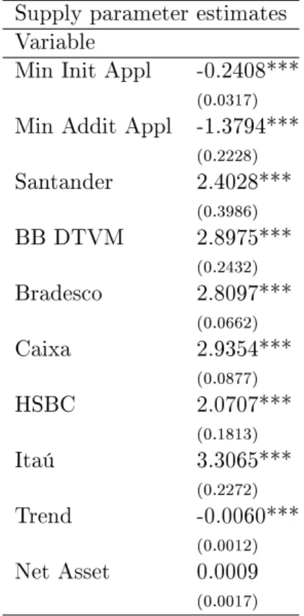
Cost parameters estimates indicate that larger minimum initial and additional applications decrease costs and that costs should decrease over time. For the minimum initial application, an increase of 10000 BRL would decrease the marginal cost in 0.2408 BRL. Unexpectedly the coefficient on the net asset is positive, however it is not significant.
Table 1.3: Supply parameter estimates Supply parameter estimates Variable
Min Init Appl -0.2408***
(0.0317)
Min Addit Appl -1.3794***
(0.2228) Santander 2.4028*** (0.3986) BB DTVM 2.8975*** (0.2432) Bradesco 2.8097*** (0.0662) Caixa 2.9354*** (0.0877) HSBC 2.0707*** (0.1813) Itaú 3.3065*** (0.2272) Trend -0.0060*** (0.0012) Net Asset 0.0009 (0.0017)
Standard Errors are reported in parentheses *** Significant at 1% level
Since larger minimum initial application decreases marginal costs, an administration fee neg-atively correlated with the minimum initial application does not necessarily indicate the presence of second-degree price discrimination.
To test for the presence of second-degree price discrimination, I calculated de markup for each fund using the estimates obtained for the marginal cost parameters.8 Then for each bank I
ob-served how it varies as minimum initial application increases. Since markups decrease with larger minimum initial applications, results suggest the presence of second-degree price discrimination.
8The markup for fund 𝑗 is given by 𝑝𝑗−𝑚𝑐𝑗
1.6 Counterfactual and Welfare Analysis
Banks offer multiple funds with negatively correlated administration fees and minimum initial applications. Results indicate that differences in marginal cost are not essential to explain differences in administration fees, which evidences a possible second-degree price discrimination by banks.
Since individuals with a lower income should invest a lower amount and therefore pay a higher price, one should be interested in evaluating how prices and therefore consumer welfare would vary if banks could not charge multiple administration fees.
For this purpose I perform two counterfactual exercises. In the first counterfactual, each bank can charge a unique administration fee for its funds, given minimum initial application observed in the data. In the second counterfactual, each bank choose a unique administration fee for its funds, given a hypothetical minimum initial application. I allow the values 100, 1000, 5000, 10000, 15000, 20000, 25000, 30000 and 35000 BRL for the minimum initial applications.
The bank can charge only one administration fee 𝑝, thus its profit function becomes
Π𝑓 = ∑︁ 𝑗∈𝒥𝑓 (𝑝 − 𝑚𝑐𝑗)𝑀 𝑠𝑗(𝑝,𝑥,𝜉; 𝜃) (1.14) with FOCs ∑︁ 𝑗∈𝒥𝑓 (︃ 𝑠𝑗(𝑝,𝑥,𝜉; 𝜃) + (𝑝 − 𝑚𝑐𝑗) 𝜕𝑠𝑗(𝑝,𝑥,𝜉; 𝜃) 𝜕𝑝 )︃ = 0 (1.15)
Which in vector notation are
(𝑠(𝑝,𝑥,𝜉; 𝜃) − ∆(𝑝,𝑥,𝜉; 𝜃). * [𝑝 − 𝑚𝑐])′* 1|𝒥
𝑓| = 0 (1.16)
where ∆𝑗(𝑝,𝑥,𝜉; 𝜃) =
𝜕𝑠𝑗(𝑝,𝑥,𝜉; 𝜃)
𝜕𝑝 and 1|𝒥𝑓| is a vector of ones with dimension equal to the
number of funds offered by bank 𝑓.
To compute the counterfactual predicted prices, I search for the price 𝑝 that solve these FOCs along with the parameters estimates from the structural model and the minimum initial
application specified.9
The upper part of Table1.4presents the predicted administration fees for each counterfactual. The last column shows the administration fees under the first scenario, which keeps the observed minimum initial application. Figure1.7shows the minimum, maximum, mean and counterfactual administration fee for each bank. As can be seen the predicted fee for each bank lies around its mean. 0 1 2 3 4 5 6 7 8 9 10 2007m1 2008m1 2009m1 2010m1 2011m1 2012m1 Date Min_Santander Mean_Santander Max_Santander Contraf_Santander 0 1 2 3 4 5 6 7 8 9 10 2007m1 2008m1 2009m1 2010m1 2011m1 2012m1 Date Min_BB Mean_BB Max_BB Contraf_BB 0 1 2 3 4 5 6 7 8 9 10 2007m1 2008m1 2009m1 2010m1 2011m1 2012m1 Date Min_Bradesco Mean_Bradesco Max_Bradesco Contraf_Bradesco 0 1 2 3 4 5 6 7 8 9 10 2007m1 2008m1 2009m1 2010m1 2011m1 2012m1 Date Min_Caixa Mean_Caixa Max_Caixa Contraf_Caixa 0 1 2 3 4 5 6 7 8 9 10 2007m1 2008m1 2009m1 2010m1 2011m1 2012m1 Date Min_HSBC Mean_HSBC Max_HSBC Contraf_HSBC 0 1 2 3 4 5 6 7 8 9 10 2007m1 2008m1 2009m1 2010m1 2011m1 2012m1 Date Min_Itaú Mean_Itaú Max_Itaú Contraf_Itaú
Figure 1.7: Minimum, maximum, mean and counterfactual administration fee for each bank Others columns show the predicted administration fee under the second counterfactual, which fixes the minimum initial application. These are given in tens of thousands of BRL and vary
from 100 BRL to 35000 BRL. Figure 1.8presents the observed minimum, maximum and mean
9The system cannot be solved analytically. Therefore I use the operator 𝑇 : R6 −→ R6 𝑇 (𝑝) = 𝑝 + 𝐷𝐼′(𝑆 + (𝜙(𝑝) − 𝑚𝑐). * 𝐸(𝑝))
where 𝑆 is the observed vector of market shares, 𝑚𝑐 is the predicted vector of marginal costs, 𝐸(𝑝) is the vector of market share derivatives with respect to price calculated in the vector of prices 𝑝, 𝜙(·) is a function that associates the price vector of each bank with the price each fund charges each period and DI is a matrix with dummies for each bank.
This operator was not proved to be a contraction, but I tried from different initial 𝑝 which lead to the same fixed point.
of minimum initial application for each bank. 0 5 10 15 20 2007m1 2008m1 2009m1 2010m1 2011m1 2012m1 Date Min_Santander Mean_Santander Max_Santander 0 5 10 15 20 2007m1 2008m1 2009m1 2010m1 2011m1 2012m1 Date Min_BB Mean_BB Max_BB 0 5 10 15 20 2007m1 2008m1 2009m1 2010m1 2011m1 2012m1 Date Min_Bradesco Mean_Bradesco Max_Bradesco 0 5 10 15 20 2007m1 2008m1 2009m1 2010m1 2011m1 2012m1 Date Min_Caixa Mean_Caixa Max_Caixa 0 5 10 15 20 2007m1 2008m1 2009m1 2010m1 2011m1 2012m1 Date Min_HSBC Mean_HSBC Max_HSBC 0 5 10 15 20 2007m1 2008m1 2009m1 2010m1 2011m1 2012m1 Date Min_Itaú Mean_Itaú Max_Itaú
Figure 1.8: Minimum, Maximum and Mean of the Minimum Initial Application for each bank For each bank the administration fee decreases monotonically with a larger initial application. Moreover, the initial application would have to be around 25000 BRL to reach the administration fee predicted with the observed initial application.
Table 1.4: Counterfactual Results
Bank Minimum Initial Application
0.01 0.1 0.5 1 1.5 2 2.5 3 3.5 -Santander 2.32 2.31 2.24 2.15 2.06 1.98 1.89 1.80 1.72 1.89 BB DTVM 2.06 2.04 1.97 1.89 1.80 1.72 1.63 1.54 1.45 1.55 Bradesco 2.44 2.43 2.36 2.27 2.18 2.10 2.01 1.92 1.84 2.11 Caixa 1.58 1.57 1.50 1.41 1.32 1.24 1.15 1.06 0.98 1.22 HSBC 2.06 2.05 1.98 1.89 1.80 1.72 1.63 1.54 1.46 1.52 Itaú 2.71 2.69 2.62 2.53 2.45 2.36 2.28 2.19 2.11 1.9
Change in Consumer Surplus
Mean -1.15 -1.11 -0.96 -0.76 -0.56 -0.36 -0.16 0.03 0.23 -0.12
Max -0.45 -0.42 -0.29 -0.13 0.04 0.20 0.37 0.54 0.71 0.30
Min -6.18 -6.10 -5.76 -5.33 -4.91 -4.48 -4.05 -3.63 -3.20 -0.86
I also compute the variation in consumer surplus for each counterfactual scenario. Consumer surplus is given by the following expression
𝐶𝑆𝑖 = ∫︁ 1 𝛼𝑖 log∑︁ 𝑗 𝑒[𝛿𝑗(𝛼,𝛽)+𝜇𝑖𝑗(𝛽𝑠,𝛽𝑑)] d𝐹 𝜈(𝜈)d𝐹𝑑(𝑑) + 𝐾 (1.17)
and therefore the change in consumer surplus is10
∆𝐶𝑆𝑖= ∫︁ 1 𝛼𝑖 {︂ log∑︁ 𝑗 𝑒[𝛿𝑗(𝛼,𝛽)+𝜇𝑖𝑗(𝛽𝑠,𝛽𝑑)]− log∑︁ 𝑗 𝑒[𝛿𝑗(𝛼,𝛽)+𝜇𝑖𝑗(𝛽𝑠,𝛽𝑑)] }︂ d𝐹𝜈(𝜈)d𝐹𝑑(𝑑) (1.18)
For this it is supposed that the coefficient 𝛼𝑖 is independent of income, which does not occur
in my specification. But as commented in Train (2003) one can use this specification when the change in consumer surplus is small relative to income.
I compute the change in consumer surplus for each consumer at each counterfactual scenario. The results are in the lower part of Table1.4. Given that consumer tastes vary, along with the mean change in consumer surplus I also present the maximum and minimum change in consumer surplus for each scenario.
For lower values of the minimum initial application, the administration fee becomes larger than observed and all consumers are in a worse situation. With a larger initial application, the loss in consumer surplus decrease but the mean variation only becomes positive from 30000 BRL. Using the observed minimum initial application, some consumers are better and others worse. However, the mean change is negative. The existence of consumers with positive and others with negative variation in utility seems reasonable as consumers that have a fund with large (low) initial application, have a low(large) administration fee which means that in the counterfactual its administration fee increase (decrease).
These results may give some advice for policy makers. Even though there is evidence that banks price discriminate, which leads consumers whose buy a lower amount (and possibly have a lower income) to pay higher fees. The attempt to prevent banks from price discriminate -imposing the same administration fee and (or) minimum initial application - almost makes a
10Actually, this integral does not has closed form and is calculated using simulation. With 𝑛𝑠 draws of individ-uals Δ𝐶𝑆𝑖= 1 𝑛𝑠 𝑛𝑠 ∑︁ 𝑖=1 1 𝛼𝑖 {︂ log∑︁ 𝑗 𝑒[𝛿𝑗(𝛼,𝛽)+𝜇𝑖𝑗(𝛽𝑠,𝛽𝑑)]− log∑︁ 𝑗 𝑒[𝛿𝑗(𝛼,𝛽)+𝜇𝑖𝑗(𝛽𝑠,𝛽𝑑)] }︂
decrease in consumer welfare. If the government wants to increase the welfare of those who buy lower amounts, it should seek through other ways.
1.7 Conclusion
This work estimated demand and supply for Brazilian fixed income funds using a structural model of consumer and pricing behavior. As expected, results indicate that administration fee decreases funds market share, higher income agents are less price sensitive, age and minimum initial application increase funds demand. Marginal cost increase over time and decrease with larger minimum initial and additional applications.
In the data administration fee and minimum initial application are negatively correlated. I use the estimates obtained to recover how much of the fee differences could not be cost explained and therefore are evidence of second-degree price discrimination. The results show that most of the fee differences are not cost explained and that markups decrease with larger minimum initial application, suggesting the presence of price discrimination.
I performed two counterfactual exercises to understand how fees would change if banks could not charge multiple fees nor minimum initial applications. The results indicate that consumers would be worse in almost situations. Therefore any regulation to mitigate banks price discrimi-nation should be viewed with prudence.
1.8 Appendix: Computational Details
The algorithm for estimation of random coefficients logit model with supply consists of an outer loop that guess different values of the parameters (Π,Σ) and an inner loop that search for the vector 𝛿 that equalizes the predicted and the observed vector of market shares.11
This consists of four steps:
1. Obtain 𝑛𝑠 draws of the individual taste vector (𝑑𝑖,𝜐𝑖)
2. Guess 𝜃2 and calculate:
11This kind of algorithm is often called a Nested Fixed Point (NFP) algorithm, following the terminology of Rust(1987).
(a) Predicted market share using 𝜃2 and 𝛿.
(b) The vector of mean values 𝛿 that equals the predicted and observed market shares using the fixed point contraction.
(c) The vector of 𝑚𝑐 from firms FOC. (d) Optimal 𝜃1 and 𝛾 using GMM.
(e) Objective function value. 3. Return to item 2.
Can Switching Costs Reduce Prices?
2.1 Introduction
In many markets consumers must incur a cost to start or stop consuming a good or service. This cost is called switching cost and can be monetary or not. For example, when opening a bank account it may be necessary to pay fees or just go to the bank and wait in line and fill roles, which possibly involve some disutility for the consumer.
Along with consumers, firms are also affected by the existence of switching costs. As described inKlemperer(1995), firms have an incentive to increase prices and exploit its current consumers, but also to reduce prices and increase the number of consumers next period. The incentive to increase prices is called harvesting incentive, while the one to decrease is called investing incentive. Therefore the net effect of switching costs on prices depends on which of these incentives prevails. In this paper I present a model of consumer and pricing behavior and use it to determine how prices, market share and profits change with different switching cost levels.
Consumers are forward-looking and choose the good that maximize its utility given their expectation on the future values of all products, which embeds that she must pay if decides to change in another period. The monopolist firm is also forward-looking and at each period chooses prices in order to maximize the present value of its profits. The firm is aware that consumer is forward-looking and also has an expectation on the future values of its products.
I solve the model numerically for different switching cost levels and the results suggest the dominance of the harvesting effect. However, prices do not monotonically increase with switching costs. Market shares and profits increase for small switching costs and decrease for larger ones, which contrasts the intuition that firms always benefits from increases in switching costs.
Additionally I show how one can estimate model’s parameters using only aggregate data. The paper adds to the literature that analyses the effect of switching costs on prices. Klem-perer(1995) presented a multi-period model with two firms and found that prices increase with switching costs, whatever their previous market share. Additionally, prices increase with the fraction of consumers that remains at each period and decrease with firms’ discount rate and new consumers entry rate.
Ho (2015) estimates the demand for consumers deposits in Chinese banks using a dynamic model of demand with switching costs. He performs counterfactual exercises with a dynamic monopoly model and finds increasing prices on switching costs and initial market shares. Viard
(2007) also found decreasing prices for lower switching costs.
Using a panel data on individual purchases of refrigerated orange juice and margarine Dube et al.(2009) estimate the switching costs. They use a model with multi-product firms and myopic consumers. Prices and profits decrease with switching costs
With a structural modelShcherbakov(2016) estimates a model of dynamic consumer behavior with switching costs in the market for paid-television services using data on cable and satellite systems across local US television markets.
The remainder of this paper is organized as follows. Section 3.2 presents the model of con-sumer and firm behaviour. Section 2.3 presents a simplified version of the model. Section 2.4
computes the model predictions for different switching cost values. Section 3.3 presents the estimation method. Section 3.5 concludes. Appendix 3.6 shows the synthetic data generating process, a numerical example and the steps of the computational procedure.
2.2 Model
The model consists of an infinitely lived multiproduct monopolist firm which sells its products for consumers with switching costs.
The firm set prices to maximize the expected present value of its profits. It has expectations about future values of its products and is aware of consumer’s problem.
Consumer chooses the product that maximizes the expected present value of her utility. Therefore in addition to her present utility, the consumer takes into account her expectation about products future utility (which also depends on firms pricing) and that she must pay a cost
for each period she changes the purchased product.
Next I formally present the consumer’s problem and obtain the aggregate demand, then firm’s problem is presented. Section3.3and Appendix3.6provide details of the estimation and computational method.
2.2.1 Consumer Problem
Consumer is infinitely lived and discounts the future at rate 𝛽. As a discrete choice model, at each period 𝑡 consumer choose one and only one product to purchase. If this product is not the same purchased last period, she must pay a switching cost 𝛾. There are 𝐽 + 1 products, wherein 𝐽 are produced by a monopolist firm and one is the outside good, which represents consumer possibility to not purchase any of firm’s products.
Each product has a utility 𝑑𝑗 that is constant over time, plus a shock 𝜂𝑗𝑡 and a price 𝑝𝑗𝑡
that varies over time. Consumer has a price disutility 𝛼 and an idiosyncratic shock 𝜖𝑖𝑗𝑡 that is
independently and identically distributed across models and time periods. The utility consumer 𝑖receives from purchasing product 𝑥𝑡∈ {0, 1, . . . , 𝐽 } at period 𝑡 is
𝑢𝑖𝑥𝑡𝑡= 𝑑𝑥𝑡 + 𝜂𝑥𝑡𝑡− 𝛼𝑝𝑥𝑡𝑡− 𝛾1[𝑥𝑡̸=𝑥𝑡−1]+ 𝜖𝑖𝑥𝑡𝑡 (2.1)
where 1[𝑥𝑡̸=𝑥𝑡−1]is an indicator function which assumes value 1 if 𝑥𝑡̸= 𝑥𝑡−1 and 0 otherwise. Let
˜
𝛿𝑗𝑡 := 𝑑𝑗 + 𝜂𝑗𝑡− 𝛼𝑝𝑗𝑡 the mean utility of product 𝑗 at period 𝑡, consumer utility can be written
as
𝑢𝑖𝑥𝑡𝑡= ˜𝛿𝑥𝑡𝑡− 𝛾1[𝑥𝑡̸=𝑥𝑡−1]+ 𝜖𝑖𝑥𝑡𝑡 (2.2)
the mean utility of the outside good is normalized to zero, i.e., ˜𝛿0𝑡= 0, ∀𝑡.
At period 𝑡 consumer has 𝐽 +1 options and chooses the product 𝑗 that maximizes the sum of expected discounted future utilities conditional on her information at 𝑡. She is aware of products utility 𝑑𝑗, shocks 𝜂𝑡, prices 𝑝𝑡, idiosyncratic shocks 𝜖𝑖𝑡 and the product purchased in the last
period 𝑥𝑡−1. But she does not have information on future values of shocks 𝜂, prices 𝑝 and
idiosyncratic shocks 𝜖.1 Additionally, define 𝛿𝑗𝑡 := ˜𝛿𝑗𝑡+ 𝛼𝑝𝑗𝑡 the product mean utility before the
price disutility.
1Notation: ˜𝛿
I assume the mean utility 𝛿 follows a Markov process, while the shocks 𝜖𝑖𝑗𝑡are independently
and identically distributed across models and time periods and follows an extreme value type one (EVT1) distribution.
The consumer state variables at period 𝑡 are (𝑥𝑡−1,𝑠𝑡−1,𝛿𝑡,𝜖𝑡). With the Markov assumption
the consumer problem can be written recursively and the time subscript 𝑡 omitted. Denote with a subscript −1 the previous period value of a variable and with a prime the next period value, the consumer value function is
𝑉 (𝑥−1,𝑠−1,𝛿,𝜖) := max 𝑥 {︁ 𝛿𝑥− 𝛼𝑝𝑥− 𝛾1[𝑥̸=𝑥−1]+ 𝜖𝑥+ 𝛽E(︀𝑉 (𝑥,𝑠,𝛿 ′,𝜖′)|𝛿)︀}︁ 𝑠.𝑡. 𝑠 = 𝜑(𝑠−1,𝛿,𝑝) 𝑝 = 𝑔(𝑠−1,𝛿) (2.3)
where 𝜑 is the market share function that comes from consumer problem and 𝑔 the firm policy function. These will be derived in the next subsections. The 𝑝𝑥 and 𝜖𝑥 are the price and
idyossincratic shock of product 𝑥, respectively.
Note that consumer choice will be one of the next period state variables and she will have to pay the switching cost 𝛾 if she changes the product. The consumer policy function is
ℎ(𝑥−1,𝑠−1,𝛿,𝜖) = arg max 𝑥 {︁ 𝛿𝑥− 𝛼𝑝𝑥− 𝛾1[𝑥̸=𝑥−1]+ 𝜖𝑥+ 𝛽E(︀𝑉 (𝑥,𝑠,𝛿 ′,𝜖′)|𝛿)︀}︁ 𝑠.𝑡. 𝑠 = 𝜑(𝑠−1,𝛿,𝑝) 𝑝 = 𝑔(𝑠−1,𝛿) (2.4)
Rust(1987) shows that when 𝜖 follows a EVT1 distribution, the integral of the value function over 𝜖 has closed form. The integrated value function for a consumer with product 𝑗 and mean utilities 𝛿 is defined as
𝐸𝑉 (𝑥−1,𝑠−1,𝛿) :=
∫︁
𝑉 (𝑥−1,𝑠−1,𝛿,𝜖) d𝐺(𝜖) (2.5)
𝐸𝑉 (𝑥−1,𝑠−1,𝛿) = log (︃ 𝑒𝛿𝑥−1−𝛼𝑝𝑥−1+𝛽E(𝐸𝑉 (𝑥−1,𝑠,𝛿′)|𝛿)+ 𝑒−𝛾 ∑︁ 𝑘̸=𝑥−1 𝑒𝛿𝑘−𝛼𝑝𝑘+𝛽E(𝐸𝑉 (𝑘,𝑠,𝛿′)|𝛿) )︃ 𝑠.𝑡. 𝑠 = 𝜑(𝑠−1,𝛿,𝑝) 𝑝 = 𝑔(𝑠−1,𝛿) (2.6)
where 𝐺(·) is the joint CDF of shocks 𝜖 and E is the conditional expectation in the information set 𝛿.
2.2.2 Aggregate Demand
One consumer that purchases some product will not pay the switching cost in the next period unless she changes to other product. FollowingMcFadden(1974) andRust(1987), the proportion of consumers that purchased 𝑘 in the previous period and then moves to product 𝑗 is
𝜔𝑗𝑘 :=
𝑒𝛿𝑗−𝛼𝑝𝑗−𝛾1[𝑗̸=𝑘]+𝛽E(𝐸𝑉 (𝑗,𝑠,𝛿′)|𝛿)
∑︀
𝑙𝑒
𝛿𝑙−𝛼𝑝𝑙−𝛾1[𝑙̸=𝑘]+𝛽E(𝐸𝑉 (𝑙,𝑠,𝛿′)|𝛿) (2.7)
The market shares are given by
𝜑(𝑠−1,𝛿,𝑝) := Ω · 𝑠−1 (2.8)
where Ω is the matrix whose 𝑗,𝑘 element is 𝜔𝑗𝑘.2 This means that product’s 𝑗 market share is
the sum among all 𝑘 existing products of the proportion of consumers that moves from product 𝑘to product 𝑗 weighted by product’s 𝑘 previous market share.
Therefore function 𝜑 provides current market share given previous market share 𝑠−1, mean
utilities 𝛿 and price 𝑝. Note this function comes from a consumer optimizing behavior which embeds that firms act according to 𝑔 and consumers know the function 𝜑.
2.2.3 Supply
There is an infinitely lived multi-product monopolist that produces 𝐽 products at each period. Firm profit at period 𝑡 is
𝜋(𝑠𝑡−1,𝛿𝑡,𝑝𝑡) = (𝑝𝑡− 𝑐𝑡) · 𝜑(𝑠𝑡−1,𝛿𝑡,𝑝𝑡)𝑀𝑡 (2.9)
where 𝑐𝑡is vector of products marginal costs at period 𝑡, 𝑀𝑡is the market size (which I normalize
to one) and 𝛿𝑡 is the vector of products mean utilities without the price disutility.
The firm is infinitely lived and at period 𝑡 chooses its products prices 𝑝𝑡in order to maximize
the sum of expected discounted future profits conditional on its information set. It is aware of previous market shares 𝑠𝑡−1, present mean utilities 𝛿𝑡 and has an expectation on its evolution.
I suppose 𝛿 follows a Markov process and therefore firm’s problem can be written recursively. Firm’s Bellman equation is
𝑊 (𝑠−1,𝛿) = max 𝑝 {︃ 𝑝 · 𝑠 + 𝛽 E (︁ 𝑊 (𝑠,𝛿′) ⃒ ⃒ ⃒𝛿 )︁ }︃ 𝑠.𝑡. 𝑠 = 𝜑(𝑠−1,𝛿,𝑝) (2.10)
the state variables are the previous market shares 𝑠−1 and the mean utilities 𝛿, while price 𝑝
is the control variable. The present market share 𝑠 is determined by equation 3.9, hence the expectation is taken only conditional on 𝛿.
The firm policy function is
𝑔(𝑠−1,𝛿) = arg max 𝑝 {︃ 𝑝 · 𝑠 + 𝛽 E(︁𝑊 (𝑠,𝛿′) ⃒ ⃒ ⃒𝛿 )︁ }︃ 𝑠.𝑡. 𝑠 = 𝜑(𝑠−1,𝛿,𝑝) (2.11)
and returns firm price 𝑝 given the state variables (𝑠−1,𝛿).
2.2.4 Equilibrium
The pair of functions (𝜑,𝑔) constitute an equilibrium of this game if there is no incentive to a one-period deviation. The pair (𝜑,𝑔) defined above satisfy this since:
1) Given the firm policy function 𝑔, for any value of the state variables (𝑥−1, 𝑠−1, 𝛿) the
optimizing consumer behavior in 2.4 results in the market share function 𝜑. Therefore it is consumers’ best response to 𝑔.
2) Given the market share function 𝜑, for any value of the state variables (𝑠−1,𝛿) the
opti-mizing firm behavior in2.11results in the policy function 𝑔. Therefore it is firm’s best response to 𝜑.
2.3 Simplified Model
In this section I present a simpler version of the model described above that I use to compute how prices, market shares and profits vary with switching costs. This simpler version is mainly motivated by the computational difficulty to obtain the functions 𝜑 and 𝑔. Extend the method to estimate the original model constitute the objective of future research.
Now consumers have expectations in the products mean utility after the price disutility ˜𝛿.3
Assuming that ˜𝛿 follows a Markov process, consumer Bellman equation becomes
𝑉 (𝑥−1,˜𝛿,𝜖) = max 𝑥 {︁ ˜𝛿𝑥− 𝛾1 [𝑥̸=𝑥−1]+ 𝜖𝑥+ 𝛽E(︀𝑉 (𝑥,˜𝛿 ′ ,𝜖)|˜𝛿)︀ }︁ (2.12)
and integrating in 𝜖 as previously done gives
𝐸𝑉 (𝑥−1,˜𝛿) = log (︃ 𝑒˜𝛿𝑥−1+𝛽E(𝐸𝑉 (𝑥−1,˜𝛿′)|˜𝛿)+ 𝑒−𝛾 ∑︁ 𝑘̸=𝑥−1 𝑒𝛿˜𝑘+𝛽E(𝐸𝑉 (𝑘,˜𝛿′)|˜𝛿) )︃ (2.13) The market share function is
𝜑(𝑠−1,˜𝛿) := Ω · 𝑠−1 (2.14)
where the 𝑗,𝑘 element of the matrix Ω is
𝜔𝑗𝑘 := 𝑒𝛿˜𝑗−𝛾1[𝑗̸=𝑘]+𝛽E(𝐸𝑉 (𝑗,˜𝛿′)|˜𝛿) ∑︀ 𝑙𝑒 ˜ 𝛿𝑙−𝛾1[𝑙̸=𝑘]+𝛽E(𝐸𝑉 (𝑙,˜𝛿′)|˜𝛿) (2.15) 3Remember that ˜𝛿 𝑗= 𝑑𝑗+ 𝜂𝑗− 𝛼𝑝𝑗, i.e., ˜𝛿 = 𝛿 − 𝛼𝑝.
The firm problem becomes 𝑊 (𝑠−1,𝛿) = max 𝑝 {︃ 𝑝 · 𝑠 + 𝛽 E(︁𝑊 (𝑠,𝛿′) ⃒ ⃒ ⃒𝛿 )︁ }︃ 𝑠.𝑡. 𝑠 = 𝜑(𝑠−1,˜𝛿) ˜ 𝛿 = 𝛿 − 𝛼𝑝 (2.16)
2.4 Model Predictions
Consumers must pay a switching cost 𝛾 if they change from the previous period product. Higher switching costs decrease consumer utility from changing the consumed product and therefore increase the likelihood to continue with the same product.
To firm’s pricing, an increase in the switching cost generates an unclear effect. For consumers that are inside, the firm has an incentive to increase prices. While for consumers at the outside good, firm would like to decrease prices and thus increase the chance of having they inside next period. If prices increase or decrease as switching costs increase, depends on which of these effects dominate.
In this section I assess how prices, market shares and profits would vary with different switch-ing cost levels. To do this I generate data on products prices and market shares for 𝑇 = 1000 periods. The price coefficient is set 𝛼 = 1.2 and switching cost 𝛾 = 4. There is a monopolist firm that produces two products with constant over time utilities 𝑑1 = 1.6 and 𝑑2 = 1.4. Appendix
2.7.1 give more details on the data generating process.
I use eleven switching cost levels ranging from 0% to 100% of the switching cost value used to generate the data. These are presented at Table2.1.
Table 2.1: Switching costs Percentage of original switching cost
0% 10% 20% 30% 40% 50% 60% 70% 80% 90% 100%
Value 0 0.4 0.8 1.2 1.6 2 2.4 2.8 3.2 3.6 4
With parameter values and the switching cost I compute the firm policy function and use it to construct a sequence of prices and market shares given one sequence of mean utilities 𝛿 draws.
I generate three hundred sequences of prices and market shares. Appendix 2.7.2 summarizes these steps.
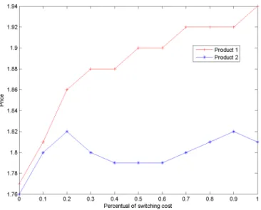
Table 2.2 shows the mean value of prices, market shares and revenues (which equals profit, since costs are normalized to zero) for each 𝛾 value.4 These are also shown in figure 2.1, figure
2.2and figure 2.3.
Table 2.2: Results
Percentage of original switching cost
0% 10% 20% 30% 40% 50% 60% 70% 80% 90% 100% Price Prod 1 1.77 1.81 1.86 1.88 1.88 1.90 1.90 1.92 1.92 1.92 1.94 Prod 2 1.76 1.80 1.82 1.80 1.79 1.79 1.79 1.80 1.81 1.82 1.81 Market Share Prod 1 0.29 0.29 0.29 0.29 0.30 0.30 0.30 0.29 0.28 0.25 0.17 Prod 2 0.24 0.24 0.24 0.26 0.26 0.26 0.26 0.25 0.24 0.22 0.15 Profit Prod 1 0.51 0.53 0.54 0.55 0.56 0.57 0.57 0.56 0.53 0.48 0.33 Prod 2 0.42 0.43 0.44 0.46 0.47 0.47 0.47 0.45 0.43 0.40 0.26
In each case there are 300 sequences of draws, with 300 periods each. The means are across the last 15 periods of all sequences.
Product 1 has a higher price than product 2 for all switching cost levels. This is expected since its constant over time utility 𝑑1 is higher than 𝑑2. Moreover, the price of product 1 is
increasing with switching costs, while the price of product 2 decreases for some switching cost levels. Market share increase for lower switching costs and decrease for larger ones. The same occurs with profits.
Therefore results suggest the dominance of the harvesting effect, although prices do not always increase with switching costs. The effect on market share suggests that larger switching costs can inhibit consumers to enter and then prefer to stay with the outside good. This decrease in profits indicate that firm does not always benefit from larger switching costs. This result comes from the hypothesis that consumers start in the outside good and probably would change if she starts consuming one of the firm’s products.
4Initial market share for both products are 0. The same results were found with initial market share 0.2, except for 𝛾 = 4 which found mean price, market share and profit for products 1 and 2 respectively, 1.94, 1.83, 0.20, 0.18, 0.39, 0.33.
Figure 2.1: Prices with different switching cost levels
Figure 2.3: Profits with different switching cost levels
2.5 Estimation Algorithm
Now I present the estimation algorithm to recover the parameters. These are the switching cost parameter 𝛾, products dummies (𝑑1, 𝑑2) and price sensibility 𝛼. The computational steps are
outlined in Appendix2.7.3.
Given a guess 𝛾 of the switching cost, guess a sequence ˜𝛿𝐽 𝑇 ∈ R𝐽 𝑇 of mean utilities. Suppose
˜
𝛿 is a process such that
˜
𝛿𝑗𝑡= 𝜇𝑗 + 𝜐𝑗𝑡 𝜐𝑗𝑡 ∼ 𝑁 (0, 𝜎𝑗2) , ∀𝑗,𝑡 (2.17)
then estimate 𝜇𝑗 and 𝜎𝑗2 using maximum likelihood to construct the grid of values that ˜𝛿𝑗𝑡 can
assume, denoted 𝑔𝑟𝑖𝑑(˜𝛿), and then the transition matrix.5 The Appendix 2.7.4 provides the
details of the grid and transition matrix computation.
Following Rust (1987) integrate consumer value function 2.12 in 𝜖 which leads to a closed form solution that simplify the estimation and compute
𝐸𝑉 (𝑥−1,˜𝛿) = log
(︃
exp𝛿˜𝑥−1+𝛽E(𝐸𝑉 (𝑥−1,˜𝛿′)|˜𝛿)+ exp−𝛾 ∑︁
𝑘̸=𝑥−1
exp𝛿˜𝑘+𝛽E(𝐸𝑉 (𝑘,˜𝛿′)|˜𝛿)
)︃
(2.18)
for all values of 𝑥 and ˜𝛿, where 𝑥 ∈ {0, 1, . . . , 𝐽} and ˜𝛿 ∈ 𝑔𝑟𝑖𝑑(˜𝛿).
Let 𝑆 = (𝑆11,𝑆21, . . . ,𝑆𝐽 1, . . . , 𝑆𝐽 𝑇) ∈ R𝐽 𝑇 be the vector of observed market shares with 𝑆𝑗𝑡
being the market share of product 𝑗 at period 𝑡. Obtain the vector of mean utilities ˜𝛿𝐽 𝑇 =
(˜𝛿11,˜𝛿21, . . . , ˜𝛿𝐽 𝑇) ∈ R𝐽 𝑇 such that predicted market shares equals observed market shares for all
products 𝑗 and time periods 𝑡, i.e.,
𝑆𝑗𝑡 = 𝜑𝑗𝑡(𝑆𝑡−1,˜𝛿𝑡) ∀𝑗,𝑡 (2.19)
where 𝜑𝑗𝑡(𝑆𝑡−1,˜𝛿𝑡) is the predicted market share of product 𝑗 at period 𝑡. Analogously toBerry
et al. (1995), given the initial ˜𝛿0 interact the system
𝑇 (˜𝛿𝐽 𝑇) = ˜𝛿𝐽 𝑇 + 𝑆 − 𝜑(𝑆,˜𝛿𝐽 𝑇) (2.20)
until obtain its fixed point, denoted ˜𝛿1.6
Once the fixed point is found, compare initial guess ˜𝛿 and ˜𝛿1. If these vectors are different
return to equation2.17and repeat all steps using ˜𝛿1. Update the mean utility vector and repeat
this process until the mean utilities are equal.
After this convergence is achieved, estimate ˆ𝑑1, ˆ𝑑2 and ˆ𝛼 using GMM
˜
𝛿𝑗𝑡 = 𝑑𝑗+ 𝜂𝑗𝑡− 𝛼𝑝𝑗𝑡 (2.21)
since prices at period 𝑡 are correlated with the shock 𝜂𝑡 correct for endogeneity using the
instru-mental variables presented in Appendix 2.7.1.
To solve firm’s problem recover 𝛿 using ˆ𝛼 and then construct 𝑔𝑟𝑖𝑑(𝛿) and 𝑔𝑟𝑖𝑑(𝑠). The details of the grid construction are provided in Appendix2.7.4. Since it is also supposed that 𝛿 follows a Markov process, it is possible to write the problem in the recursive form and obtain firm’s value and policy functions. For each 𝛿𝑛∈ 𝑔𝑟𝑖𝑑(𝛿) and 𝑠𝑚 ∈ 𝑔𝑟𝑖𝑑(𝑠)obtain
𝑊 (𝑠−1,𝑚,𝛿𝑛) = max 𝑝 {︃ 𝑝 · 𝑠 + 𝛽 E (︁ 𝑊 (𝑠,𝛿′) ⃒ ⃒ ⃒𝛿 )︁ }︃ 𝑠.𝑡. 𝑠 = 𝜑(𝑠−1,𝛿,𝑝) (2.22)
6I found fast convergence by iterating period by period. Which means, given ˜𝛿
𝑜𝑙𝑑𝑡, interact until find the mean utility that equalizes the predicted and observed market share for the period 𝑡 and then turn to 𝑡 + 1.
with the policy function 𝑔(𝑠−1,𝛿)compute the vector ˆ𝑝(𝛾) ∈ R𝐽 𝑇 of predicted prices given 𝑆 and
˜
𝛿𝐽 𝑇, therefore calculate ||𝑝 − ˆ𝑝(𝛾)||.
Then guess another 𝛾 and repeat all the procedure. The estimated switching cost ˆ𝛾 is such that
ˆ
𝛾 = arg min
𝛾 ||𝑝 − ˆ𝑝(𝛾)|| (2.23)
2.6 Conclusion
This paper analyzed how prices, market shares and profits behave in a market with switching costs. In the model consumers are infinitely lived and must pay a switching cost to change the purchased product, while the monopolist firm is also infinitely lived and choose prices to maximize profits.
Results do not support the predictions fromKlemperer(1995) that prices are increasing with switching costs. However, there is a dominance of the harvesting effect. Market shares and profits of both products increase for lower switching costs and decrease for larger ones.
2.7 Appendix
2.7.1 Synthetic Data-Generating Process
To estimate the model I generate a synthetic data which consists of 𝑇 = 1000 periods and 𝐽 = 2 products. Products have a constant over time utilities 𝑑1 = 1.6 and 𝑑1 = 1.4, the switching cost
is 𝛾 = 4 and the price coefficient 𝛼 = 1.2. The prices follow
𝑝1𝑡= 𝑝1+ 𝜂1𝑡+ 𝜐1𝑡
and
where 𝑝1 = 1.34 and 𝑝2 = 1.16. The shocks are distributed as 𝜂𝑗𝑡 𝑖𝑖𝑑∼ 1/4 · 𝑁 (0,1) and 𝜐𝑗𝑡 𝑖𝑖𝑑∼
1/4 · 𝑁 (0,1).
I simulate instrumental variables to correct for the endogeneity of prices in equation 2.21. Since these are correlated with the shocks 𝜂𝑗𝑡 as shown in the equations above.
Denote 𝑧𝑗𝑡 the vector of instruments for product 𝑗 at period 𝑡, these are 𝑑1, 𝑑2, 𝑝𝑗 + 𝜅𝑗𝑡,
(𝑝𝑗+ 𝜅𝑗𝑡)2 , (𝑝𝑗+ 𝜅𝑗𝑡)3 and 𝜐𝑗𝑡, where 𝜅𝑗𝑡 𝑖𝑖𝑑
∼ 1/4 · 𝑁 (0,1).
Previous market share in 𝑡 = 1 is 𝑠0 = (0.2,0.2)and equation3.9is used to generate the data
for the next periods {(𝑠1𝑡,𝑠2𝑡,𝑝1𝑡,𝑝2𝑡)}𝑇𝑡=1. 2.7.2 Algorithm
With 𝑑1, 𝑑2, 𝛼 and 𝛾 I evaluate how prices and market shares would change with different 𝛾. It
consists of the following steps: 1. Set one switching cost 𝛾𝑐.
2. Compute 𝐸𝑉 (𝑥−1,˜𝛿) , ∀𝑥−1∈ {0, 1, . . . , 𝐽 } and ∀˜𝛿 ∈ 𝑔𝑟𝑖𝑑(˜𝛿).
3. Solve firm’s problem to obtain its new policy function 𝑔𝑐(𝑠−1,𝛿).
4. Guess initial state variables (𝛿1,𝑠0), use 𝑔𝑐 and consumer market share function to obtain
the vector of prices and market share for period 1.
(a) Draw 𝛿2 and use 𝑠1 to obtain prices and market share for the period 2.
(b) Calculate the corresponding sequence of prices and market shares.
(c) Return to item 4 and given the same initial state variables repeat the process with another sequence of 𝛿 draws.
2.7.3 Estimation Steps
The estimation algorithm used was written in MATLAB and consists of the following steps: 1. Guess a switching cost 𝛾.
2. Obtain ˜𝛿 that equals the predicted and observed market share. (a) Initial guess of ˜𝛿0 , with 𝑔𝑟𝑖𝑑(˜𝛿0).
(b) Compute transition matrix for consumer, given ˜𝛿0 and 𝑔𝑟𝑖𝑑(˜𝛿0).
(c) Compute 𝐸𝑉 (𝑥−1,˜𝛿) , ∀𝑥 ∈ {0, 1, . . . , 𝐽} and ∀˜𝛿 ∈ 𝑔𝑟𝑖𝑑(˜𝛿0).
(d) Obtain the vector of mean utilities ˜𝛿 that equals the predicted and observed market shares.
(e) If ˜𝛿0 ̸= ˜𝛿: ˜𝛿 becomes ˜𝛿0, update 𝑔𝑟𝑖𝑑(˜𝛿0) and return to (𝑏). Else go to 3.
3. Estimate parameters ˆ𝑑1, ˆ𝑑2 and ˆ𝛼 using GMM.
4. Obtain 𝛿 = ˜𝛿0+ ˆ𝛼𝑝and construct 𝑔𝑟𝑖𝑑(𝛿).
5. Solve firm’s problem to obtain its policy function 𝑔(𝑠−1,𝛿).
6. Calculate the vector of predicted prices according to h, denoted by ˆ𝑝(𝛾). 7. Compute the objective function ||𝑝 − ˆ𝑝(𝛾)||.
8. Return to item 1.
9. Repeat 8 until find a global minimum of the objective function.
2.7.4 Grid and Transition Matrix
The products’ mean utility ˜𝛿𝑗𝑡 follows
˜
𝛿𝑗𝑡 = 𝜇𝑗+ 𝜀𝑗𝑡
where 𝜀𝑗𝑡 𝑖𝑖𝑑
∼ 𝑁 (0,𝜎2). Given a ˜𝛿 sequence, use maximum likelihood to estimate
ˆ 𝜇𝑗 = 1/𝑇 ·∑︀𝑡˜𝛿𝑗𝑡 and ˆ 𝜎𝑗 = (︁ 1/𝑇 ·∑︀ 𝑡(˜𝛿𝑗𝑡− ˆ𝜇𝑗)2 )︁1/2
the parameters of the normal distribution and then construct 𝑔𝑟𝑖𝑑(˜𝛿).
Mean utilities ˜𝛿𝑗 assume the values {˜𝛿𝑗1, ˜𝛿𝑗2, . . . , ˜𝛿𝑗𝐷} in the grid , with ˜𝛿𝑗𝑘 < ˜𝛿𝑗𝑘+1. Then
˜
˜
𝛿𝑗𝑘 = 𝐹−1(︀(2 · 𝑘 − 1)/2𝐷)︀
where 𝐹 (·) is the CDF of a normal distribution with mean ˆ𝜇𝑗 and standard deviation ˆ𝜎𝑗.
There-fore the transition probability of product 𝑗 from state 𝑘 to 𝑙 is
P(𝛿˜𝑗𝑘|˜𝛿𝑗𝑙) = 1/𝐷
2.7.5 Numerical Example
I use the estimation procedure from Section 3.3and the synthetic generated dataset to recover the switching cost 𝛾, products dummy (𝑑1, 𝑑2) and price sensibility 𝛼.
Table 2.3 reports the results. The parameters values used to generate the data are in the second column, while the estimated values and objective function value are in the third column. Estimated coefficients have the true sign and lie around the true value.
Table 2.3: Results
Variable True Estimate
Switching Cost (𝛾) 4 4
Price (𝛼) 1.2 1.14
Dummy Product 1 (𝑑1) 1.6 1.75
Dummy Product 2 (𝑑2) 1.4 1.21
Estimating an oligopoly model with
differentiated goods and two-part tariffs
3.1 Introduction
Many markets are characterized by a pricing scheme composed of two parts: an entry or access fee and a constant price charged at each period of consumption. In Economics this is known as a two-part tariff.1 It is used to price discriminate across heterogeneous consumers, allowing oligopolistic
firms to further extract the consumer surplus. Examples of this practice include investment funds and health clubs which sometimes charge an entry or membership fee in addition to the periodic administration fee.
We adapt the environment from Berry et al. (1995) in which heterogeneous firms act in a price-setting oligopolistic market with heterogeneous consumers. In the demand side, represented by a random coefficients logit model, consumers differ from each other in the length of time they intend to consume the service. They have different valuations for observed characteristics of the service and for its per-period cost (which depends on the regular price, the entry fee, and the number of periods of consumption.) In the supply side, oligopolistic firms choose entry fees and regular prices for an exogenously given set of services with different characteristics.
We derive firms’ market shares and optimal conditions taking into account the use of an entry fee to price discriminate across heterogeneous consumers. We then adjust the mathematical programming with equilibrium constraints (MPEC) method used and discussed in Dubé et al.
1The two-part tariff also comprises the case with continuous demand, in which the consumer pays a membership fee and a per-unit price (rather than a per-period fee). Although similar in spirit, we do not consider the details of this case here.