Sampling grids used to characterise the spatial variability of pH, Ca, Mg and V in Oxisols

(1)

www.ccarevista.ufc.br _{ISSN 1806-6690}

Sampling grids used to characterise the spatial variability of pH, Ca,

Mg and V% in Oxisols

1

Malhas amostrais utilizadas na caracterização da variabilidade espacial de pH, Ca,

Mg e V% em Latossolos

Maurício Roberto Cherubin2_{*, Antônio Luis Santi}3_{, Mateus Tonini Eitelwein}4_{, Clovis Orlando Da Ros}3_{e Mateus}

Bortoluzi Bisognin5

ABSTRACT - Knowledge of spatial variability is an important factor to be considered in planning a program of soil sampling and crop management under precision agriculture (PA). In this context, the aim of this work was to evaluate the efficiency of the dimensions of sampling grids used in the state of Rio Grande do Sul (RS), Brazil to characterise the spatial variability of the attributes pH_water, base saturation (V%), calcium (Ca) and magnesium (Mg) levels. The study was carried out on 30 agricultural sites located in the northern region of RS, having soils classified as Oxisols and managed using the tools of PA. The dimensions of the grids under study were: 100 x 100 m (10 areas), 142 x 142 m (10 areas) and 173 x 173 m (10 areas). Soil was collected at a depth of 0.00 to 0.10 m. The data for pH_water, V%, Ca and Mg were subjected to exploratory statistical analysis and to geostatistical analysis by means of semivariograms. The areas showed high Ca (>4.0 cmol_c dm-3_{) and Mg (>1.0 cmol}

c dm-3) levels and localised problems of soil acidity (pH_water <5.5 or V<65%), justifying the carrying out of liming at specific sites. For the geostatistical procedures, the sample grids used at the sites of the Oxisols managed under PA in RS are not efficient in capturing the scales of spatial variability of the attributes pH_water, V%, Ca and Mg, which could compromise the accuracy of corrective prescriptions for specific sites.

Key words: Soil acidity. Precision Agriculture. Soil sampling. Geostatistics.

RESUMO - O conhecimento da variabilidade espacial é um importante fator a ser considerado no planejamento de um programa de amostragem de solo e manejo das culturas na agricultura de precisão (AP). Nesse contexto, o objetivo do trabalho foi avaliar a eficiência das dimensões das malhas amostrais utilizadas no Rio Grande do Sul (RS) na caracterização da variabilidade espacial dos atributos pH_água, saturação por bases (V%), teores de cálcio (Ca) e magnésio (Mg). O estudo foi realizado em 30 áreas agrícolas localizadas na região Norte do RS que apresentam solos classificados como Latossolos Vermelhos e que são manejadas com ferramentas de AP. As dimensões das malhas amostrais estudadas foram: 100 x 100 m (10 áreas), 142 x 142 m (10 áreas) e 173 x 173 m (10 áreas). A profundidade de coleta de solo foi de 0,00-0,10 m. Os dados de pH_água, V%, Ca e Mg foram submetidos à análise estatística exploratória e à análise geoestatística por meio de semivariogramas. As áreas apresentaram elevados teores de Ca (> 4,0 cmol_c dm-3_{) e Mg (> 1,0 cmol}

c dm-3) e problemas localizados de acidez (pHágua < 5,5 ou V < 65%), justificando a realização de calagem em sítios específicos. Considerando os procedimentos geoestatísticos, as malhas amostrais utilizadas nas áreas de Latossolos Vermelhos manejados com AP no RS não são eficientes para captar as escalas da variabilidade espacial dos atributos de pH_água, V%, teores de Ca e Mg, podendo comprometer a acurácia das prescrições de corretivos em sítios específicos. Palavras-chave:Acidez do solo. Agricultura de precisão. Amostragem de solo. Geoestatística.

*Autor para correspondência

1_{Recebido para publicação em 26/03/2013; aprovado em 24/06/2014}

Parte da Dissertação de Mestrado do primeiro autor, apresentada ao Programa de Pós-Graduação em Agronomia: Agricultura e Ambiente da Universidade de Santa Maria, campus Frederico Westphalen, RS

2_{Programa de Pós-Graduação em Solos e Nutrição de Plantas, Escola Superior de Agricultura “Luiz de Queiroz”, Universidade de São}

Paulo-ESALQ/USP, Piracicaba-SP, Brasil, [email protected]

3_{Departamento de Ciências Agronômicas e Ambientais, Centro de Educação Superior Norte do Rio Grande do Sul, Universidade Federal de Santa}

Maria, Frederico Westphalen-RS, Brasil, [email protected], [email protected]

4_{Programa de Pós-Graduação em Engenharia de Sistemas Agrícolas, ESALQ/USP, Piracicaba-SP, Brasil, [email protected]} 5_{Graduando em Agronomia, Centro de Educação Superior Norte do Rio Grande do Sul, Universidade Federal de Santa Maria, Frederico}

(2)

INTRODUCTION

Oxisols are widely distributed across almost all regions of Brazil, and make up the predominant taxonomic class, occupying 31.61% of the surface of

the country (2.69 million km2_{) (ANJOS}_{et al}_{., 2012). In}

the state of Rio Grande do Sul (RS), Oxisols occur mainly in the north, a region located in the geomorphic province of the Plateau, formed by a succession of volcanic flows, followed by cooling on the surface of the earth’s crust and the formation

of predominantly basaltic rocks (STRECKet al., 2008).

These are weathered, deep, well-drained and acidic soils and display high homogeneity in the profile

(ANJOS et al., 2012; MONTANARI et al., 2008;

STRECKet al., 2008). However, despite being considered

homogeneous soils, they may comprise variations in their characteristics over both short and long distances.

Variability of the soil is a result of the interaction of complex pedogenic processes controlled by factors in its formation such as climate, topography, source material and vegetation, and intensified by land-use and management practices (MALLARINO; WITTRY, 2004). Understanding spatial variability in the soil is therefore a factor that should be considered when planning a program of soil sampling and of crop management (KERRY; OLIVER; FROGBROOK, 2010; MALLARINO; WITTRY, 2004;

MONTANARI et al., 2008; MONTANARIet al., 2012;

NANNI et al., 2011; SOUZA et al., 2004; STEPIEN;

GOZDOWSKI; SAMBORSKI, 2013).

With the advent of precision agriculture (PA) in Brazil and especially in the South region, where only in RS state, it is estimated that approximately two million hectares are

managed using tools of PA (SANTIet al., 2009), knowledge

of the spatial variability of the soil was made possible through systematic sampling by means of regular grids. However, although the use of sampling grids is officially recommended in the South of Brazil (COMISSÃO DE QUÍMICA E FERTILIDADE DO SOLO, 2004), there are still doubts as to the ideal size which would allow capture of the spatial variability of the chemical properties of the soil.

Currently, the sampling grids that are commonly adopted on Brazilian farms have dimensions ranging

from 100 to 225 m (NANNIet al., 2011). In the South

region, samples are collected at somewhat smaller distances, from 100 to175 m. However, the definition of such dimensions for the grids is primarily based on economic and practical reasons and sometimes neglects the geostatistical principles of spatial dependence (VIEIRA, 2000; WEBSTER; OLIVER, 2007).

The influence that the dimensions of the grids used in collecting soil samples have on the accuracy of the generated information is widely discussed in international

literature. Studies involve the use of the principles and tools of geostatistics to direct the sampling of soils (KERRY; OLIVER; FROGBROOK, 2010; WEBSTER; LARK, 2012), the influence of the size of the sampling grid on the quality of data interpolation (KRAVCHENKO 2003; FRANZEN, 2011), the reproducibility of the spatial

variability (CHANGet al., 1999; STEPIEN; GOZDOWSKI;

SAMBORSKI, 2013) and the management of nutrients at specific sites (MALLARINO; WITTRY, 2004; STEPIEN; GOZDOWSKI; SAMBORSKI, 2013). However, there are few studies on the conditions of Brazilian soils

(MONTANARIet al., 2012; NANNIet al., 2011) and none

for conditions in the South of Brazil.

In this context, the aim of this work was to evaluate the efficiency of the dimensions of sampling grids used in RS in characterising the spatial variability of the attributes pH_water and V% and Ca and Mg levels in Oxisols under PA.

MATERIAL AND METHODS

The study was carried out in 30 agricultural areas located in 13 municipalities in the north of Rio Grande do Sul, Brazil (Figure 1), covering 2,467.82 ha. The study area is located in the geomorphic province of the Plateau , and

extends to the physiographic regions of theAlto Uruguai,

Planalto MédioandMissões. The terrain is gently undulating

with the predominant soils classified as Oxisols (Latossolos

Vermelhosby Brazilian Classification Soil System), having

high aluminum and iron levels associated with a low base saturation (alumino ferric, dystroferric or dystrophic) and

clayey texture (STRECKet al., 2008).

The management system that has been adopted in the area is direct planting (no-tillage), rotating soybean and maize crops in the summer and white oats, black oat and forage turnip in the winter. Fertilization is carried out in the sowing furrow for each crop, and liming over the total area every five years or so.

The areas were sampled from the dimensions of the grids that are commonly used at field level in the south of Brazil, these being: 100 x 100 m (one sample for each ha); 142 x 142 m (one sample for every two ha); and 173 x 173 m (one sample for every three ha). Thus, for each grid 10 areas were studied, giving a total of 1,461 soil samples. The areas being analysed were sampled for the first time by georeferencing, so they did not suffer the effects of previous variable-rate applications of lime and fertilizer.

(3)

Figure 1 - Location of the study area, highlighting the 13 municipalities where are located the 30 agricultural areas of Oxisols, managed under precision farming

(COMISSÃO DE QUÍMICA E FERTILIDADE DO SOLO, 2004) for agricultural areas under consolidated no-tillage systems. The samples were later forwarded to the laboratory where basic chemical analyses were conducted following methodologies recommended by the Commission for Chemistry and Soil Fertility (2004). The following attributes were evaluated in the

study: active acidity (pH_water, 1:1), base saturation (V%)

and the cations related to acidity: calcium (Ca, cmol_c dm-3₎

and magnesium (Mg, cmol_c dm-3_).

Data were subjected to descriptive statistical analysis using the Statistical Analysis System - SAS 8.0 software (SAS Inc, Cary, USA), with the aim of verifying position and dispersion of the data. The statistical parameters determined were; minimum; mean; maximum; standard deviation and coefficients of variation (CV%), precision (CP%), skewness (Cs) and kurtosis (Ck). Based on the CV values obtained, the dispersion of the data was

classified as low (CV < 15%), moderate (CV 15-35%) and high (CV > 35%) (WILDING; DREES, 1983). In addition, the existence of a central tendency (normality) in the original data was noted using the W-test (p<0.05).

Analysis of the spatial variability of the pH_water

data, V%, Ca and Mg, was carried out by semivariogram, adjusted by theoretical mathematical models using the Gamma Design Software - GS+. The models for the semivariogram were adjusted based on the best

coefficient of determination (r2_{) and lowest residual}

sum of squares (RSS), and were evaluated using cross validation. The parameters of the semivariogram were defined from the adjustment of a mathematical model

to the data: nugget effect (C₀), contribution (C₁), sill

(C₀ + C1) and range (a). The spatial dependence index (SDI)

was calculated using the relationship shown in Equation 1.

(4)

The degree of spatial dependence (DSD), based on the SDI, was classified as strong for SDI 25%; moderate for an SDI between 25 and 75%, and weak

for SDI> 75% (CAMBARDELLAet al. 1994).

RESULTS AND DISCUSSION

Exploratory statistical analysis of the attributes

for pH_água and V% (Table 1) made it possible to verify

that 27 areas studied (90.0%) present places with problems of soil acidity, pH <5.5 or V <65.0%, which can restrict normal plant development under no-tillage system (COMISSÃO DE QUÍMICA E FERTILIDADE DO SOLO, 2004). This finding is related to the natural acidity characteristic of soils that have undergone intense weathering, and associated with processes of soil acidification triggered by the management practice

adopted (ANJOSet al., 2012; STRECKet al., 2008). In

agricultural areas, soil acidity is enhanced by absorption of the base cations by crops and their subsequent export at harvest, by inadequate soil management favouring the erosion and exposure of (more acidic) subsurface horizons, by the use of nitrogen fertilizers and by the oxidation of sulphur and organic matter (SOUZA; MIRANDA; OLIVEIRA, 2007).

The use of smaller sampling grids, allowing for an increase in the number of sampling points, resulted in improvements in the representativeness and accuracy of soil sampling conducted in the study areas (<% CP). However, irrespective of the grid dimensions, it was possible to identify, based

on the minimum and maximum values for pH_água

and V%, a considerable amplitude relative to the mean, demonstrating that the use of georeferenced soil sampling, as recommended under PA, was characterised as an important strategy in identifying places where soil acidity may become a limiting factor. Thus, PA allows an increase in the technical and economic efficiency of the use of limestone, based on interventions located at a specific site.

It was found that for dispersion of the data, based on the coefficient of variation (CV%), the values

for pH_water showed low dispersion (CV: <15%), with an

amplitude of from 2.06 to 7.76%. Whereas the values for %V ranged from 3.92 to 25.18%, classifying the dispersion as from low to moderate (CV: <35%). These results agree with several studies made into Oxisols

(BOTTEGA et al., 2013; CHERUBIN et al., 2011;

DALCHIAVON et al., 2012; LIMA; SILVA; SILVA,

2013; MONTANARIet al., 2008; SANTIet al., 2012;

SOUZAet al., 2004). However, the low CVs seen for

the values of pH_water are due to its logarithmic scale of

expression, requiring caution in comparison with other variables (SOUZA; MIRANDA; OLIVEIRA, 2007).

Although the data for pH_water and V% displayed low

and moderate dispersion, 56.66 and 26.66% of the areas studied did not follow normal frequency distributions, being confirmed by coefficients of skewness, offset to the left (Cs <0) or to the right (Cs> 0), and by coefficients of kurtosis with platykurtic (Ck <0) and leptokurtic (Ck> 0) distributions. Results like these, that indicate a lack of normality in the data, were also seen in areas

of Oxisols by Cavalcante et al. (2007), Cherubin et al.

(2011), Dalchiavon et al. (2012) and Montanari et al.

(2008). However, it is important to note that normality of the data is not a requirement of geostatistics; but the presence of a skewed distribution having many anomalous values should be considered, since kriging is a linear estimator (WEBSTER; OLIVER, 2007). In geostatistics, more important than the normality of the data is whether or not the so-called proportional effect occurs, in which the mean and variance of the data may not be constant, nor be a function of spatial positioning in the study area

(CAVALCANTEet al., 2007).

For the Ca and Mg cations (Table 2), it was found that the Oxisols studied display on average levels considered as high for both of these macronutrients (Ca >

4.0 cmol_c dm-3_{and Mg > 1.0 cmol}

c dm-3) (COMISSÃO DE

QUÍMICA E FERTILIDADE DO SOLO, 2004).

In studies conducted by Amado et al. (2009),

Cherubin et al. (2011) and Santi et al. (2012) into

Oxisol in RS, high levels of Ca and Mg were also found, agreeing with the results of the present work. These high levels are due to the weathering of minerals rich in these elements, such as plagioclase, pyroxene and olivine, in the makeup of the basalt rocks which are the predominant source material of the Oxisol

occurring in the study region (STRECK et al., 2008).

Furthermore, the addition of dolomitic limestone over the years, associated with the low mobility of the Ca and Mg in the soil, may also have significantly contributed to the maintenance and rise in levels of these macronutrients.

Dispersion of the Ca and Mg data was classified as low to moderate, with CV amplitudes that ranged from 11.94 to 34.08% and from 14.86 to 35.00% respectively,

agreeing with Amado et al. (2009), Bottega et al.

(2013), Cavalcantiet al. (2007), Cherubinet al. (2011),

Lima, Silva and Silva (2013), Santi et al. (2012) and

Souzaet al. (2004). Normal frequency distributions for

(5)

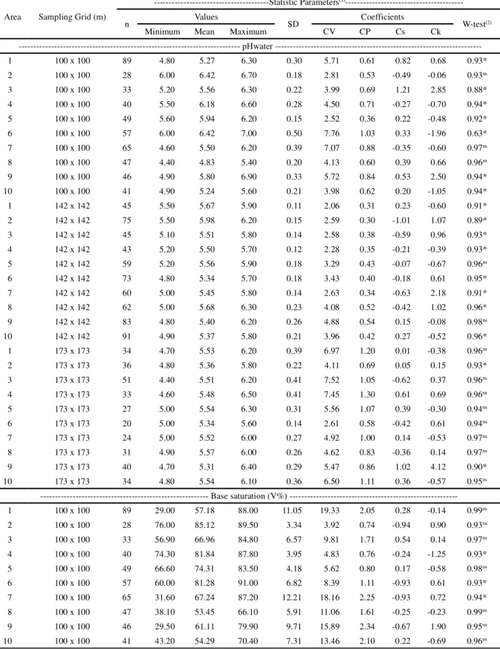
Table 1 - Descriptive statistics of the attributes for pH_water and base saturation (V%) in Oxisols areas sampled with different dimensions of sampling grid

Area Sampling Grid (m)

---Statistic Parameters(1)

---n Values SD Coefficients W-test(2)

Minimum Mean Maximum CV CP Cs Ck

--- pHwater

---1 100 x 100 89 4.80 5.27 6.30 0.30 5.71 0.61 0.82 0.68 0.93*

2 100 x 100 28 6.00 6.42 6.70 0.18 2.81 0.53 -0.49 -0.06 0.93ns

3 100 x 100 33 5.20 5.56 6.30 0.22 3.99 0.69 1.21 2.85 0.88*

4 100 x 100 40 5.50 6.18 6.60 0.28 4.50 0.71 -0.27 -0.70 0.94*

5 100 x 100 49 5.60 5.94 6.20 0.15 2.52 0.36 0.22 -0.48 0.92*

6 100 x 100 57 6.00 6.42 7.00 0.50 7.76 1.03 0.33 -1.96 0.63*

7 100 x 100 65 4.60 5.50 6.20 0.39 7.07 0.88 -0.35 -0.60 0.97ns 8 100 x 100 47 4.40 4.83 5.40 0.20 4.13 0.60 0.39 0.66 0.96ns

9 100 x 100 46 4.90 5.80 6.90 0.33 5.72 0.84 0.53 2.50 0.94*

10 100 x 100 41 4.90 5.24 5.60 0.21 3.98 0.62 0.20 -1.05 0.94*

1 142 x 142 45 5.50 5.67 5.90 0.11 2.06 0.31 0.23 -0.60 0.91*

2 142 x 142 75 5.50 5.98 6.20 0.15 2.59 0.30 -1.01 1.07 0.89*

3 142 x 142 45 5.10 5.51 5.80 0.14 2.58 0.38 -0.59 0.96 0.93*

4 142 x 142 43 5.20 5.50 5.70 0.12 2.28 0.35 -0.21 -0.39 0.93*

5 142 x 142 59 5.20 5.56 5.90 0.18 3.29 0.43 -0.07 -0.67 0.96ns

6 142 x 142 73 4.80 5.34 5.70 0.18 3.43 0.40 -0.18 0.61 0.95*

7 142 x 142 60 5.00 5.45 5.80 0.14 2.63 0.34 -0.63 2.18 0.91*

8 142 x 142 62 5.00 5.68 6.30 0.23 4.08 0.52 -0.42 1.02 0.96*

9 142 x 142 83 4.80 5.40 6.20 0.26 4.88 0.54 0.15 -0.08 0.98ns

10 142 x 142 91 4.90 5.37 5.80 0.21 3.96 0.42 0.27 -0.52 0.96*

1 173 x 173 34 4.70 5.53 6.20 0.39 6.97 1.20 0.01 -0.38 0.96ns

2 173 x 173 36 4.80 5.36 5.80 0.22 4.11 0.69 0.05 0.15 0.93*

3 173 x 173 51 4.40 5.51 6.20 0.41 7.52 1.05 -0.62 0.37 0.96ns 4 173 x 173 33 4.60 5.48 6.50 0.41 7.45 1.30 0.61 0.69 0.96ns 5 173 x 173 27 5.00 5.54 6.30 0.31 5.56 1.07 0.39 -0.30 0.94ns 6 173 x 173 20 5.00 5.34 5.60 0.14 2.61 0.58 -0.42 0.61 0.94ns 7 173 x 173 24 5.00 5.52 6.00 0.27 4.92 1.00 0.14 -0.53 0.97ns 8 173 x 173 31 4.90 5.57 6.00 0.26 4.62 0.83 -0.36 0.14 0.97ns

9 173 x 173 40 4.70 5.31 6.40 0.29 5.47 0.86 1.02 4.12 0.90*

(6)

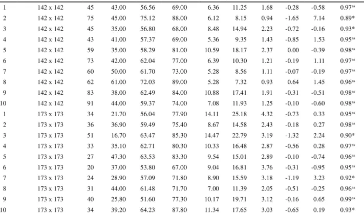
1 142 x 142 45 43.00 56.56 69.00 6.36 11.25 1.68 -0.28 -0.58 0.97ns 2 142 x 142 75 45.00 75.12 88.00 6.12 8.15 0.94 -1.65 7.14 0.89* 3 142 x 142 45 35.00 56.80 68.00 8.48 14.94 2.23 -0.72 -0.16 0.93* 4 142 x 142 43 41.00 57.37 69.00 5.36 9.35 1.43 -0.85 1.53 0.95ns 5 142 x 142 59 35.00 58.29 81.00 10.59 18.17 2.37 0.00 -0.39 0.98ns 6 142 x 142 73 42.00 62.04 77.00 6.39 10.30 1.21 -0.19 1.11 0.97ns 7 142 x 142 60 50.00 61.70 73.00 5.28 8.56 1.11 -0.07 -0.19 0.97ns 8 142 x 142 62 61.00 72.03 89.00 5.28 7.32 0.93 0.64 1.45 0.96ns 9 142 x 142 83 38.00 62.49 84.00 10.88 17.41 1.91 -0.31 -0.51 0.98ns 10 142 x 142 91 44.00 59.37 74.00 7.08 11.93 1.25 -0.10 -0.60 0.98ns 1 173 x 173 34 21.70 56.04 77.90 14.11 25.18 4.32 -0.73 0.33 0.95ns 2 173 x 173 36 36.90 59.49 75.40 8.67 14.58 2.43 -0.18 0.27 0.98ns 3 173 x 173 51 16.70 63.47 85.30 14.47 22.79 3.19 -1.32 2.24 0.90* 4 173 x 173 33 35.10 62.71 80.30 10.33 16.48 2.87 -0.56 0.28 0.97ns 5 173 x 173 27 47.30 63.53 83.30 9.54 15.01 2.89 -0.10 -0.74 0.96ns 6 173 x 173 20 37.00 53.80 67.00 9.04 16.81 3.76 -0.31 -0.95 0.95ns 7 173 x 173 24 28.90 57.09 71.80 8.90 15.59 3.18 -1.19 3.23 0.92* 8 173 x 173 31 44.00 61.48 71.70 7.00 11.39 2.05 -0.51 -0.25 0.96ns 9 173 x 173 40 25.80 51.60 77.30 10.17 19.71 3.12 -0.16 0.65 0.99ns 10 173 x 173 34 39.20 64.23 87.80 11.34 17.65 3.03 -0.65 0.19 0.93*

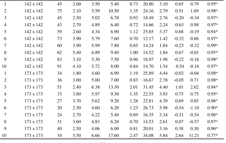
Table 2 - Descriptive statistics for the calcium (Ca - cmol_c dm-3_{) and magnesium (Mg - cmol}

c dm-3) levels in Oxisols areas sampled with different dimensions of sampling grid

Table 1 continued

(1)_{n: number of observations (sampling points); SD: standard deviation; CV(%): coeficient of variation; CP (%): coefficient of precision; Cs:}

coefficient of skewness; Ck: coefficient of kurtosis;(2)_{W-test: Shapiro-Wilk test for normal distribution, where: (*) significant at levels of}

p<0.05 and (ns) not significant. When significant, indicates that the normal distribution hypothesis is rejected

Área Sampling Grid (m)

Statistic Parameters(1)

n Values SD Coefficients W-test(2)

Minimum Mean Maximum CV CP Cs Ck

Calcium

---1 100 x 100 89 2.70 5.26 9.90 1.15 21.82 2.31 1.01 2.40 0.95*

2 100 x 100 28 5.30 9.07 10.80 1.24 13.71 2.59 -1.34 1.95 0.89*

3 100 x 100 33 6.10 7.62 10.20 0.83 10.88 1.89 0.75 1.59 0.96ns

4 100 x 100 40 5.50 7.94 10.00 1.15 14.46 2.29 0.29 -0.66 0.94*

5 100 x 100 49 4.50 6.91 11.30 1.07 15.50 2.21 1.40 5.12 0.91*

6 100 x 100 57 4.50 7.88 13.50 1.77 22.48 2.98 0.99 1.99 0.93*

7 100 x 100 65 3.60 6.76 10.20 1.20 17.82 2.21 -0.04 1.33 0.97ns

8 100 x 100 47 4.90 6.45 8.30 0.77 11.94 1.74 0.29 -0.10 0.98ns

9 100 x 100 46 1.70 3.34 5.30 0.81 24.31 3.58 0.52 0.17 0.97ns

(7)

Table 2 continued

1 142 x 142 45 2.00 3.50 5.40 0.73 20.80 3.10 0.65 0.79 0.95ns

2 142 x 142 75 2.10 5.59 10.50 1.35 24.16 2.79 0.51 1.69 0.98ns

3 142 x 142 45 2.50 5.02 6.70 0.93 18.49 2.76 -0.20 -0.34 0.97ns

4 142 x 142 43 2.70 4.89 6.40 0.72 14.66 2.24 -0.63 0.98 0.97ns

5 142 x 142 59 2.60 4.34 6.90 1.12 25.85 3.37 0.68 -0.19 0.94*

6 142 x 142 73 3.90 5.79 7.60 0.70 12.17 1.42 -0.32 0.86 0.97ns

7 142 x 142 60 3.90 5.99 7.80 0.85 14.24 1.84 -0.23 -0.32 0.99ns

8 142 x 142 62 5.40 6.89 9.40 1.00 14.52 1.84 0.67 -0.01 0.95*

9 142 x 142 83 3.10 5.30 7.50 0.96 18.07 1.98 -0.22 -0.16 0.98ns

10 142 x 142 91 4.10 5.72 8.00 0.84 14.70 1.54 0.54 -0.16 0.97ns

1 173 x 173 34 1.80 4.60 6.90 1.19 25.89 4.44 -0.02 -0.04 0.98ns

2 173 x 173 36 3.00 5.00 7.00 0.83 16.67 2.78 -0.05 0.71 0.98ns

3 173 x 173 51 2.40 6.38 13.30 2.01 31.45 4.40 1.01 2.62 0.94*

4 173 x 173 33 3.80 5.97 9.30 1.35 22.55 3.93 0.75 0.75 0.95ns

5 173 x 173 27 3.70 5.62 9.20 1.28 22.81 4.39 0.69 0.85 0.96ns

6 173 x 173 20 2.50 4.60 6.20 1.23 26.73 5.98 -0.54 -1.10 0.90*

7 173 x 173 24 2.70 4.22 5.40 0.69 16.35 3.34 -0.31 -0.54 0.96ns

8 173 x 173 31 3.60 4.83 6.20 0.70 14.53 2.61 0.07 -0.57 0.97ns

9 173 x 173 40 2.50 4.06 6.00 0.81 20.01 3.16 0.38 0.30 0.96ns

10 173 x 173 34 3.50 6.66 17.60 2.47 34.08 5.84 2.64 11.21 0.77*

Magnesium

---1 100 x 100 89 0.90 2.26 6.00 0.72 31.70 3.36 1.93 7.41 0.86*

2 100 x 100 28 1.50 3.01 3.60 0.50 16.54 3.13 -1.56 2.43 0.84*

3 100 x 100 33 2.40 3.16 4.90 0.49 15.54 2.71 1.31 3.57 0.91*

4 100 x 100 40 2.20 3.46 4.60 0.61 17.66 2.79 -0.01 -0.41 0.96ns

5 100 x 100 49 1.60 2.40 3.70 0.36 14.97 2.14 0.92 2.80 0.94*

6 100 x 100 57 1.60 3.30 4.80 0.63 18.98 2.51 0.24 0.18 0.97ns

7 100 x 100 65 1.00 2.24 3.40 0.53 23.63 2.93 -0.12 -0.16 0.98ns

8 100 x 100 47 1.20 2.12 3.30 0.40 18.91 2.76 0.50 0.82 0.96ns

9 100 x 100 46 0.70 1.55 2.90 0.49 31.71 4.68 0.97 0.87 0.92*

10 100 x 100 41 1.30 2.02 3.00 0.43 21.10 3.30 0.95 0.19 0.89*

1 142 x 142 45 0.90 1.52 2.60 0.36 23.74 3.54 1.19 1.71 0.91*

2 142 x 142 75 1.00 2.68 5.00 0.64 24.01 2.77 0.58 1.75 0.96*

3 142 x 142 45 0.80 1.99 3.20 0.52 26.16 3.90 0.33 0.06 0.97ns

4 142 x 142 43 0.60 1.59 2.30 0.32 20.29 3.09 -0.40 1.36 0.95ns

5 142 x 142 59 1.00 1.86 3.90 0.58 31.13 4.05 1.25 1.74 0.90*

6 142 x 142 73 1.70 2.69 5.90 0.75 27.98 3.27 2.92 9.60 0.65*

7 142 x 142 60 1.50 2.29 3.80 0.41 17.77 2.29 0.81 2.04 0.96*

8 142 x 142 62 1.70 2.81 3.80 0.46 16.19 2.06 -0.08 -0.32 0.99ns

9 142 x 142 83 1.20 2.13 3.20 0.48 22.50 2.47 -0.05 -0.55 0.98ns

(8)

(1)_{n: number of observations (sampling points); SD: standard deviation; CV(%): coeficient of variation; CP (%): coefficient of precision; Cs:}

coefficient of skewness; Ck: coefficient of kurtosis;(2)_{W-test: Shapiro-Wilk test for normal distribution, where: (*) significant at levels of}

p<0.05 and (ns) not significant. When significant, indicates that the normal distribution hypothesis is rejected

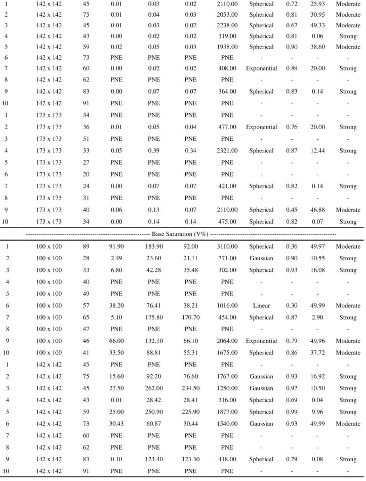
Table 3 - Geostatistical analysis of the attributes for pH_water and base saturation (V%) in Oxisols areas sampled with different dimensions of sampling grid

Area Sampling Grid (m) n Nugget Effect Sill Contribution Range Model r2 Spatial Dependence SDI(1) _DSD(2)

--- pH_água

---1 100 x 100 89 PNE(3) _PNE _PNE _PNE _- _- _-

-2 100 x 100 28 0.00 0.06 0.05 636.00 Linear 0.98 8.10 Strong

3 100 x 100 33 0.04 0.05 0.01 422.80 Linear 0.30 78.00 Weak

4 100 x 100 40 0.05 0.11 0.06 1295.00 Spherical 0.74 45.45 Moderate

5 100 x 100 49 PNE PNE PNE PNE - - -

-6 100 x 100 57 PNE PNE PNE PNE - - -

-7 100 x 100 65 0.00 0.17 0.17 397.00 Spherical 0.98 1.49 Strong

8 100 x 100 47 0.00 0.04 0.04 246.00 Exponential 0.69 2.50 Strong 9 100 x 100 46 0.04 0.12 0.08 384.00 Exponential 0.77 33.33 Moderate 10 100 x 100 41 0.01 0.04 0.03 442.00 Spherical 0.99 22.32 Strong

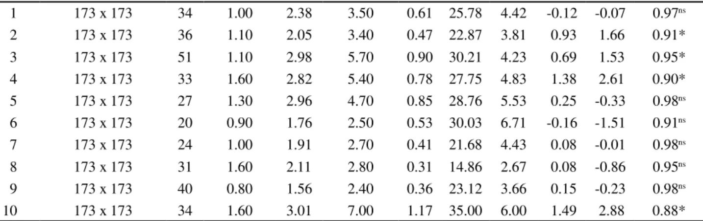
1 173 x 173 34 1.00 2.38 3.50 0.61 25.78 4.42 -0.12 -0.07 0.97ns

2 173 x 173 36 1.10 2.05 3.40 0.47 22.87 3.81 0.93 1.66 0.91*

3 173 x 173 51 1.10 2.98 5.70 0.90 30.21 4.23 0.69 1.53 0.95*

4 173 x 173 33 1.60 2.82 5.40 0.78 27.75 4.83 1.38 2.61 0.90*

5 173 x 173 27 1.30 2.96 4.70 0.85 28.76 5.53 0.25 -0.33 0.98ns

6 173 x 173 20 0.90 1.76 2.50 0.53 30.03 6.71 -0.16 -1.51 0.91ns

7 173 x 173 24 1.00 1.91 2.70 0.41 21.68 4.43 0.08 -0.01 0.98ns

8 173 x 173 31 1.60 2.11 2.80 0.31 14.86 2.67 0.08 -0.86 0.95ns

9 173 x 173 40 0.80 1.56 2.40 0.36 23.12 3.66 0.15 -0.23 0.98ns

10 173 x 173 34 1.60 3.01 7.00 1.17 35.00 6.00 1.49 2.88 0.88*

Table 2 continued

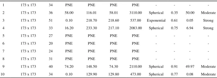
The spatial variability of the attributes pH_water

and V%, and of the bases Ca and Mg, was analysed from the results of the geostatistical analysis (Tables 3 and 4). In the four attributes studied, a large difference in the structure of spatial variability was seen for the areas under study, even when the samples were collected with the same dimensions of sampling grid. This variation can be evidenced by the amplitude observed for the radius of spatial dependence between samples (ranges). For all the grids under study, areas were noted

where the values for pH_water, V%, Ca and Mg showed

no spatial dependence, featuring random distributions (pure nugget effect), and where geostatistics therefore could not be applied (VIEIRA, 2000). Note that there is a trend towards an increase in the occurrence of random distributions as the size of the sampling grid increases, confirming assumptions of Cambardella

et al. (1994), Vieira (2000) and Webster and Oliver

(9)

Table 3 continued

1 142 x 142 45 0.01 0.03 0.02 2110.00 Spherical 0.72 25.93 Moderate 2 142 x 142 75 0.01 0.04 0.03 2053.00 Spherical 0.81 30.95 Moderate 3 142 x 142 45 0.01 0.03 0.02 2238.00 Spherical 0.67 49.33 Moderate

4 142 x 142 43 0.00 0.02 0.02 319.00 Spherical 0.81 0.06 Strong

6 142 x 142 73 PNE PNE PNE PNE - - -

-7 142 x 142 60 0.00 0.02 0.02 408.00 Exponential 0.89 20.00 Strong

8 142 x 142 62 PNE PNE PNE PNE - - -

10 142 x 142 91 PNE PNE PNE PNE - - -

-1 173 x 173 34 PNE PNE PNE PNE - - -

3 173 x 173 51 PNE PNE PNE PNE - - -

5 173 x 173 27 PNE PNE PNE PNE - - -

-6 173 x 173 20 PNE PNE PNE PNE - - -

8 173 x 173 31 PNE PNE PNE PNE - - -

-9 173 x 173 40 0.06 0.13 0.07 2110.00 Spherical 0.45 46.88 Moderate

--- Base Saturation (V%)

---1 100 x 100 89 91.90 183.90 92.00 3110.00 Spherical 0.36 49.97 Moderate

2 100 x 100 28 2.49 23.60 21.11 771.00 Gaussian 0.90 10.55 Strong 3 100 x 100 33 6.80 42.28 35.48 302.00 Spherical 0.93 16.08 Strong

4 100 x 100 40 PNE PNE PNE PNE - - -

-5 100 x 100 49 PNE PNE PNE PNE - - -

-6 100 x 100 57 38.20 76.41 38.21 1016.00 Linear 0.30 49.99 Moderate

8 100 x 100 47 PNE PNE PNE PNE - - -

-9 100 x 100 46 66.00 132.10 66.10 2064.00 Exponential 0.79 49.96 Moderate

1 142 x 142 45 PNE PNE PNE PNE - - -

-2 142 x 142 75 15.60 92.20 76.60 1767.00 Gaussian 0.93 16.92 Strong

3 142 x 142 45 27.50 262.00 234.50 1250.00 Gaussian 0.97 10.50 Strong 4 142 x 142 43 0.01 28.42 28.41 316.00 Spherical 0.69 0.04 Strong

5 142 x 142 59 25.00 250.90 225.90 1877.00 Spherical 0.99 9.96 Strong 6 142 x 142 73 30.43 60.87 30.44 1540.00 Gaussian 0.93 49.99 Moderate

7 142 x 142 60 PNE PNE PNE PNE - - -

-8 142 x 142 62 PNE PNE PNE PNE - - -

(10)

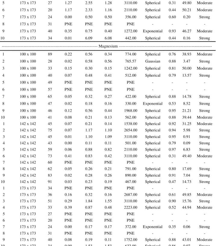
-Table 4 - Geostatistical analysis of calcium (Ca - cmol_c dm-3_{) and magnesium (Mg - cmol}

c dm-3) in Oxisol areas sampled with different dimensions of sampling grid

Área Sampling Grid (m) n Nugget Effect Sill Contribution Range Model r2 Spatial Dependence SDI(1) _DSD(2)

--- Calcium

2 100 x 100 28 0.46 3.54 3.08 843.50 Gaussian 0.87 12.99 Strong

5 100 x 100 49 PNE(3) _PNE _PNE _PNE _- _- _-

7 100 x 100 65 0.01 1.57 1.56 354.00 Exponential 0.77 0.64 Strong

8 100 x 100 47 0.38 0.77 0.39 433.00 Exponential 0.41 49.35 Moderate

10 100 x 100 41 PNE PNE PNE PNE - - -

5 142 x 142 59 0.58 1.87 1.29 553.00 Gaussian 0.97 31.02 Moderate

7 142 x 142 60 PNE PNE PNE PNE - - -

10 142 x 142 91 PNE PNE PNE PNE - - -

-(1)_{SDI: spatial dependence index;}(2)_{DSD: degree of spatial dependence;}(3)_{PNE: pure nugget effect}

1 173 x 173 34 PNE PNE PNE PNE - - -

5 173 x 173 27 PNE PNE PNE PNE - - -

-6 173 x 173 20 PNE PNE PNE PNE - - -

-7 173 x 173 24 PNE PNE PNE PNE - - -

-8 173 x 173 31 PNE PNE PNE PNE - - -

(11)

2 173 x 173 36 PNE PNE PNE PNE - - -

-3 173 x 173 51 2.92 11.85 8.93 3164.00 Gaussian 0.67 24.64 Strong

4 173 x 173 33 PNE PNE PNE PNE - - -

8 173 x 173 31 PNE PNE PNE PNE - - -

-- Magnesium

5 100 x 100 49 PNE PNE PNE PNE - - -

-6 100 x 100 57 PNE PNE PNE PNE - - -

7 142 x 142 60 PNE PNE PNE PNE - - -

1 173 x 173 34 PNE PNE PNE PNE - - -

5 173 x 173 27 PNE PNE PNE PNE - - -

-6 173 x 173 20 PNE PNE PNE PNE - - -

8 173 x 173 31 PNE PNE PNE PNE - - -

Table 4 continued

(12)

are employed in areas under PA. For Brazilian conditions, the results of the present study agree with those obtained by

Corá and Beraldo (2006) and Nanniet al. (2011) in which

the collection of one sample per hectare was not sufficient to capture the spatial variability of V%, with the use of denser grids being necessary in order to make more accurate recommendations for soil correctors possible.

Thus, in the absence of spatial dependence of the data, or with dependencies of limited reliability, it is suggested that users of PA exercise caution when employing kriging interpolation, otherwise the thematic maps of soil attributes, used to determine the variable rates of correctors and fertilizers, will not express the main patterns of spatial variability present in the area (KERRY; OLIVER, 2008). Under such conditions, the use of simple interpolation (linear or polynomial) such as inverse distance, can be just as effective as the kriging method (KRAVCHENKO, 2003; FRANZEN, 2011). According to Corá and Beraldo (2006), map accuracy is dependent on the interpolation method

used to estimate the values for non-sampled locations,

and in turn, the interpolation method is dependent on the density of sampled points per area.

These results endorse what is currently being practised in the field, where users of PA, during the preparation process for thematic maps, employ computer software available in the market, but which do not take into account the spatial dependence of the attributes being analysed in estimating values at non-sampled locations (CORÁ; BERALDO, 2006). However, it is important to state again that the ability

to generate thematic maps for the attributes pH_water, V%,

Ca and Mg in the absence of any spatial dependence of the data verified by geostatistics, does not exempt the planning of sampling from recommending denser sampling, which would be capable of actually detecting the different scales of spatial variability of the analysed attributes. As good as the interpolation method is, it will never be able to predict values with accuracy, compared to the values obtained by sampling in the field.

Given the results of this exploratory study, the

assumptions already outlined by Chang et al. (1999)

and Stepien, Gozdowski and Samborski (2013) can be confirmed, in which the spatial variability of the

attributes pH_water, V%, Ca and Mg is unique for each

area, being conditioned at different scales by intrinsic and extrinsic soil factors. Therefore, from sampling grids with dimensions 100 m, such as those that have been used in the south of Brazil, it is not possible to generalise a reliable model of the spatial variability of these attributes for Oxisols. However, the study does give an overview of the scale of variation for the soil attributes under study, and becomes an important

In areas where the attributes pH_water, V%, Ca and

Mg present a defined structure of spatial variability, it was generally found that the degree of spatial dependency was moderate to strong, showing that under such conditions, these attributes were more affected by intrinsic properties of the soil (CAMBARDELLA

et al., 1994). Furthermore, management practices,

such as the uniform surface liming carried out over the period of agricultural land use, contribute to the low spatial variability of the attributes of acidity over shorter distances.

These results however warrant caution, since the semivariograms were generated using a limited number of points (n). Webster and Lark (2012) explain that the use of 30 to 50 pairs of points over each distance, as indicated by some authors (LANDIM, 2006), means having less than 50 sampling points in two-dimensional grids and almost inevitably leads to estimates which are only slightly accurate and to semivariograms with high levels of error. According to these authors, for reliable estimates to be generated when the variation is isotropic, at least 100 sampling points are required and ideally 150 to 200.

Moreover, although the number of sampling points is considered to be important in the literature, it is not subject to generalisation for all situations, and may be too small in areas where the variables display their variability on smaller scales (short distances), and too large for areas where their variability is presented on larger scales (long distances) (KERRY; OLIVER; FROGBROOK, 2010).

When larger sampling grids are used therefore, with more widely-spaced points (usually 100 m), together with a reduced size for the areas (a situation commonly seen in the areas under PA in southern Brazil) the comprehension and representation of the different scales of variability for the attributes of acidity and related cations (Ca and Mg) are still limited, even with the use of geostatistics. It can therefore be inferred that the sampling grids used in the Oxisol areas in RS managed under PA are not efficient in capturing the different scales of spatial

variability for pH_water, V%, Ca and Mg, especially when

expressed over short distances. However, it is important to note that the insertion of PA and consequently of soil sampling with grids, even if displaying limited levels of reliability in some situations, has enabled progress to be made in diagnosing soil fertility which is unprecedented in the agriculture of Rio Grande do Sul and in the rest of Brazil, redeeming the role of sampling in the management of soil fertility and agricultural production.

(13)

reference that can assist in planning future soil sampling strategies to be adopted in areas under PA in RS.

A suggestion for the future would be carrying out detailed studies in a microregion, farm or field scale to test different dimensions for sampling grids, with a view to better understanding the variability of the different soil chemical attributes, and the possible definition of more efficient strategies for fertility management.

CONCLUSIONS

1. The sampling grids used in Oxisols under PA in RS, generally employing geostatistical procedures, are not efficient in capturing the scales of spatial

variability of the attributes pH_water, V%, Ca and Mg,

and may lead less accurate liming;

2. Spatial variability over short distances should be taken into consideration in future plans for soil sampling, aiming for the characterization and the site specific management of soil acidity in Oxisols areas managed under PA.

REFERENCES

AMADO, T. J. C. et al. Atributos químicos e físicos de Latossolos e sua relação com os rendimentos de milho e feijão irrigados.Revista Brasileira de Ciência do Solo, v. 33, n. 4, p. 831-843, 2009.

ANJOS, L. H. C. dos.et al. Sistema Brasileiro de Classificação de Solo.In: KER, J. C.et al. (Ed.).Pedologia: Fundamentos. Viçosa-MG: Sociedade Brasileira de Ciência do Solo, 2012. p. 303-343.

BOTTEGA, E. L.et al. Variabilidade espacial de atributos do solo em sistema de semeadura direta com rotação de culturas no cerrado brasileiro.Revista Ciência Agronômica, v. 44, n. 1, p. 1-9, 2013.

CAMBARDELLA, C. A.et al. Field-scale variability of soil properties in central Iowa soils.Soil Science Society American Journal, v. 58, n. 5, p. 1501-1511, 1994.

CAVALCANTE, E. G. S. et al. Variabilidade espacial de atributos químicos do solo sob diferentes usos e manejos.Revista Brasileira de Ciência do Solo, v. 31, n. 6, p. 1329-1339, 2007. CHANG, J. et al. Precision Farming Protocols: Part 1. Grid distance and soil nutrient impact on the reproducibility of spatial variability measurements.Precision Agriculture, v. 1, n. 3, p. 277-289, 1999.

CHERUBIN, M. R. et al. Caracterização e estratégias de manejo da variabilidade espacial dos atributos químicos do solo utilizando a análise dos componentes principais. Enciclopédia Biosfera, v. 7, n. 13, p. 196-210, 2011.

COMISSÃO DE QUÍMICA E FERTILIDADE DO SOLO. Manual de adubação e calagem para os estados do Rio Grande do Sul e Santa Catarina. Porto Alegre: Sociedade Brasileira de Ciência do Solo - Núcleo Regional Sul, 2004. 400 p.

CORÁ, J. E.; BERALDO, J. M. G. Variabilidade espacial de atributos do solo antes e após calagem e fosfatagem em doses variadas na cultura de cana-de-açúcar. Engenharia Agrícola, v. 26, n. 2, p. 374-387, 2006.

DALCHIAVON, F. C.et al. Variabilidade espacial de atributos da fertilidade de um Latossolo Vermelho Distroférrico sob Sistema Plantio Direto.Revista Ciência Agronômica, v. 43, n. 3, p. 453-461, 2012.

FRANZEN, D. W. Collecting and analyzing soil spatial information using kriging and inverse distance. In: CLAY, D. E.; SHANAHAN, J. F.GIS Applications in Agriculture: Nutrients Management for Energy Efficiency, USA: CRC Press, 2011. p. 61-80.

KERRY, R.; OLIVER, M. A. Determining nugget:sill ratios of standardized variograms from aerial photographs to krige sparse soil data.Precision Agriculture, v. 9, n. 1/2, p. 33-56, 2008.

KERRY, R.; OLIVER, M. A.; FROGBROOK, Z. L. Sampling in Precision Agriculture. In: OLIVER, M. A. (Org.). Geostatistical Applications for Precision Agriculture. Heidelberg: Springer-Verlag, 2010. p. 35-63.

KRAVCHENKO, A. N. Influence of spatial structure on accuracy of interpolation methods. Soil Science Society of America Journal, v. 67, n. 5, p. 1564-1571, 2003.

LANDIM, P. M. B. Sobre Geoestatística e mapas. TERRÆ DIDATICA,v. 2, n. 1, p. 19-33, 2006.

LIMA, J. S. S.; SILVA, S. A.; SILVA, J. M. Variabilidade espacial de atributos químicos de um Latossolo Vermelho-Amarelo cultivado em plantio direto. Revista Ciência Agronômica, v. 44, n. 1, p. 16-23, 2013.

MALLARINO, A. P.; WITTRY, D. Efficacy of grid and zone soil sampling approaches for site-specific assessment of phosphorus, potassium, pH, and organic matter. Precision Agriculture, v. 5, n. 2, p. 131-144, 2004.

MONTANARI, R. et al. Variabilidade espacial de atributos químicos em Latossolo e Argissolos.Ciência Rural, v. 38, n. 5, p. 1266-1272, 2008.

MONTANARI, R.et al. The use of scaled semivariograms to plan soil sampling in sugarcane fields. Precision Agriculture, v. 13, n. 5, p. 542-552, 2012.

NANNI, M. R. et al. Optimum size in grid soil sampling for variable rate application in site-specific management.Scientia Agrícola, v. 68, n. 3, p. 386-392, 2011.

(14)

SANTI, A. L. et al. É chegada a hora da integração do conhecimento. Revista Plantio Direto, v. 129, n. 1, p. 24-30, 2009.

SOUZA, D. M. G.; MIRANDA, L. N.; OLIVEIRA, S. A. Acidez do solo e sua correção.In: NOVAIS, R. F.et al. (Ed.). Fertilidade do Solo. Viçosa-MG: Sociedade Brasileira de Ciência do Solo, 2007. p. 206-274.

SOUZA, Z. M. de. et al. Variabilidade espacial do pH, Ca, Mg e V% do solo em diferentes formas do relevo sob cultivo de cana-de-açúcar.Ciência Rural, v. 34, n. 6, p. 1763-1771, 2004.

STEPIEN, M.; GOZDOWSKI, D.; SAMBORSKI, S. A case study on the estimation accuracy of soil properties and fertilizer rates for different soil-sampling grids. Journal of Plant Nutrition and Soil Science, v. 176, n. 1, p. 57-68, 2013.

STRECK, E. V. et al. Solos do Rio Grande do Sul. 2. ed. Porto Alegre: EMATER/RS-ASCAR, 2008. 222 p.

VIEIRA, S. R. Geoestatística em estudos de variabilidade espacial do solo. In: NOVAIS, R. F.; ALVARES V., V. H.; SCHAEFFER, C. E. G. R. (Ed.).Tópicos em Ciência do Solo. Sociedade Brasileira de Ciência do Solo, p. 1-54, 2000. v. 1. WEBSTER, R.; LARK, M. Field Sampling for Environmental Science and Management. London: Routledge, 2012. 200 p.

WEBSTER, R.; OLIVER, M. A. Geostatistics for Environmental Scientists. 2. ed. Chichester: John Wiley & Sons Ltd. 2007. 330 p.