• Nenhum resultado encontrado

Grid-based representation and dynamic visualization of ionospheric tomography

N/A
N/A
Protected

Academic year: 2017

Share "Grid-based representation and dynamic visualization of ionospheric tomography"

Copied!
6
0
0

Texto

(1)

GRID-BASED REPRESENTATION AND

DYNAMIC VISUALIZATION OF IONOSPHERIC TOMOGRAPHY

L. M. He a, *, Y. Yang a, C. Su a, J. Q. Yu b, F. Yang a, L. X. Wu a, b

a

Institute for Geo-informatics & Digital Mine Research, College of Resources and Civil Engineering, Northeastern

University, 110819 Shenyang, China, -

heliming@mail.neu.edu.cn

b

School of Environment Science and Spatial Informatics, China University of Mining and Technology, 221008

Xuzhou, China -

awulixin@263.net

KEY WORDS: Ionospheric tomography, Spatial grids, Dynamic visualization, Global navigation satellite system

ABSTRACT:

The ionosphere is a dynamic system with complex structures. With the development of abundant global navigation satellite systems, the ionospheric electron density in different altitudes and its time variations can be obtained by ionospheric tomography technique using GNSS observations collected by the continuously operating GNSS tracking stations distributed over globe. However, it is difficult to represent and analyze global and local ionospheric electron density variations in three-dimensional (3D) space due to its complex structures. In this paper, we introduce a grid-based system to overcome this constraint. First, we give the principles, algorithms and procedures of GNSS-based ionospheric tomography technique. Then, the earth system spatial grid (ESSG) based on the spheroid degenerated octree grid (SDOG) is introduced in detail. Finally, more than 400 continuously operating GNSS receivers from the International GNSS Service are utilized to realize global ionospheric tomography, and then the ESSG is used to organize and express the tomography results in 4D, including 3 spatial dimensions and time.

1. INTRODUCTION

The ionosphere is one of the important layers of the Earth's atmosphere, which begins near 50 km in altitude and extends to and merges with the magnetosphere at about 1000 km in altitude. It has serious influences on the propagation of electromagnetic waves, global navigation satellite system, InSAR measurement, space weather and so on. Therefore, study of ionosphere is important for many scientific fields. Generally, the ionosphere is composed of three main parts: the D, E, and F regions. The D region extends from 50 to 90 km, the E region extends from 90 to 150 km, and the F region comprises the remaining portion of the ionosphere from 150 to 1000 km. The lowest region of F region is dominated by photochemistry and known as the F1 region. The higher region of F region near the peak electron concentration profile corresponds to a transition from photochemical dominance to diffusion dominance, and is called the F2 region. But the boundaries between regions are not well-defined, and vary with ionospheric conditions (Kelley, 2009). With the rapid development of global navigation satellite system and ionosphere sounding technology, GNSS-based three-dimensional reconstruction of the ionospheric electron density technology: ionospheric tomography technology, is becoming an efficient and reliable method for ionospheric electron density analysis and modeling. Based on a large number of receivers and GNSS satellites, we can obtain the time-dependent three-dimensional (3D) distribution of ionospheric electron density using ionospheric tomography technology (Kamp, 2013, Allain and Mitchell, 2010). However, it is difficult to represent and analyze global and local ionospheric variations in 3D space due to its complex structures.

3D spatial grids based on the sphere degenerated octree grid (SDOG), devoting to solve the insufficient of traditional map projection on sphere spatial data management and the inadequate spatial dimension of spherical discrete grids, is an excellent tool for unity modelling of time-dependent 3D data (Wu and Yu,

2009a). In this paper, we use the 3D spatial grids to represent the 3D distribution of ionospheric tomography in different layers, and realize the further comprehensive visualization analysis of the ionospheric electron density obtained by ionospheric tomography technology.

2. IONOSPHERIC TOMOGRAPHY

Ionospheric tomography is a technique to monitor the ionospheric electron density in different heights based on integrated electron density. The integrated electron density can be called as total electron content (TEC), which is observed along satellite-receiver signal paths. After that, an inversion process is used to reconstruct the electron density distribution in different altitudes of the ionosphere (Kunitsyn and Tereshchenko, 2003). The abundant of GNSS signals, including GPS, GLONASS, COMPASS and GALILEO, can be applied to reconstruct an ionospheric image in 4D, including 3 spatial dimensions and time.

2.1 STEC derived from GPS measurements

The slant total electron content (STEC) in the line of sight (LOS) direction can be defined as

= ∫ (1) According to the carrier phase model equation (Misra and Enge, 2006), we can obtain the ionospheric delay of carrier phase measurements as follow:

1

2 2 1

2 2 40.28 =

40.28 =

I STEC

f

I STEC

f

(2)

Then, the can be calculated by: 2 2

1 2

1 1 2 2 1 1 2 2

2 2

1 2

[( ) ( )]

40.28(f f )

STEC N N

f f

   

   

 (3)

International Archives of the Photogrammetry, Remote Sensing and Spatial Information Sciences, Volume XL-4/W2, 2013 ISPRS WebMGS 2013 & DMGIS 2013, 11 – 12 November 2013, Xuzhou, Jiangsu, China

(2)

Taking the code phase observations (C/A code and P code) into account, the integrated ambiguous integer number of cycles can be calculated by (Mannucci et al., 1998):

1 1 2 2 2 1 1 1 2 2

1 1

1

m

(

)

1

m

(

)

i i

i i

Amb

N

N

m

m

 

 

(4)

A non-negligible error source in computing absolute STEC is induced by the different travel time of the GPS signal on the two separate frequencies through the analogue hardware of satellite and receiver respectively, which produced a constant STEC bias. If we define the relative delay on the satellite as , and the delay caused by the receiver as , the corrected STEC can be represented as:

2 2 1 2

1 1 2 2 1 1 2 2

2 2

1 2

( )

40.28(f f ) sat rec

STEC N N cT cT

f f

  

     

 (5)

2.2 Coefficient matrix setup

Ionospheric tomography based on GNSS uses a series of STECs to inverse the temporal and spatial distribution of ionospheric electron density. The first step of the inversion procedure is to determine the reconstruction region and discretize the electron density. The reconstruction region can be divided into × pixel grids in latitude and altitude, respectively. We suppose the electron density is uniformly distributed in every pixel grid. Then the electron density can be discretized by finite series-expansion reconstruction method. Let’s suppose ( , ) is the electron density in one pixel grid, and are the coordinates in a polar coordinate system. p is the propagation path of the i-thGNSS signal, the observation y is integral of electron density along p, the total number of signals is equal to . The observation equation is:

( , )

1,2,...,

i

n

i i p

P

y

f r

ds e i

N

(6)

Where e is the noise of observations.

After discretization, we obtain the following equation:

Y AX e

 

(7)

Where A is the coefficient matrix consisted of intercepts, which are GNSS signals pass through the divided pixel grids. Y is the STEC observations vector consisted of the TEC along each GNSS signal propagation path; X is the unknown parameter vector consisted of the electron density of each pixel grid; e is the noise vector of observations (Yao et al., 2013).

2.3 MART algorithm

GNSS-based computerized ionospheric tomography lack of horizontal scanning ray in the reconstruction of electron density because of the poor geometry constituted by GNSS satellites and ground receivers. In addition, because of the number of ground receivers are limited which makes the project data incomplete. The two reasons that result in the coefficient matrix A is a huge sparse and rank deficient matrix. Therefore, the equation (7) cannot be solved by the common method. The most commonly used algorithm is multiplication algebraic reconstruction technique (MART). An advantage for MART is that we still can obtain good inversion result in the case of incomplete project data (Wen et al., 2011).

This paper uses MART algorithm to reconstruct the distribution of ionospheric electron density. The ionospheric empirical model (IRI-2007) is used to set an initial electron density value of iteration for each pixel within the reconstruction region. Then the iterative approach is used to improve the initial estimation of the

reconstructed image until the improved values satisfy the minimum norm condition (Jin and Park, 2007). For the k-th iteration, the formula of MART is:

1

(

)

,

k ij i

a a

k k i

j j T k

i

y

x

x

a x

(8)

Where

1

k j

x

is the (k+1)-th iteration value of the j-th pixel vector; ij

a

is projection coefficient matrix elements; T i

a

is the

transpose of row i of A. k is iterations,

kis relaxation factor, i

y

is the TEC values of i-th path.

The characteristics of MART algorithm can be summarized as follow: each initial value should be greater than 0. In the iterative process, if a pixel value becomes 0, it still equal to 0 in the following iterative process. In the allocation of error, it will allocate the relative residuals to each component proportionally. Only one line of coefficient matrix elements are used in each iteration, thus it can save a lot of storage space. In addition, the speed of convergence of MART is fast, generally the number of iterations is less than ten times and the results are positive. It is one of the most important contents to create the iteration formula in tomography algorithm. Therefore, the iterative formula is established carefully in order to get a better reconstruct result in this paper.

2.3.1 Basis function selection

The selection of basis function will directly affect the amount of calculation of reconstruction algorithm. A complex basis function causes the amount of computation increases exponentially and reduces the computational efficiency. Therefore, we should choose a basis function which is simple and favour of calculation, further, its linear combination can be a good approximation of the reconstruct images (Yang, 2012). Strive to achieve the balance between reconstruction speed and reconstruction quality. Sometimes we need some of the constraints according to the characteristics of the image and the projection data to accelerate the convergence speed in the reconstructed image when using MART. Therefore, the basis function should overcome these constraints in order to help accelerate the convergence speed .The reconstruction area is divided into N non-overlapping pixel grid. In this paper, the following basis function is used:

1

( , )

-( , )

0

j

if r

locate in j th pixel

b r

otherwise

 

(9)

The proportion of the non-zero elements of the projection matrix is small that can be used to simplify calculations.

2.3.2 The estimation of optimal iterations

MART reconstruction is a loop iteration process. It is worth noting that the reconstruction quality is not proportional to the number of iterations. However, when it reaches a certain number of iterations, and then the reconstruction quality of the image will decline if it continues to iterate. Therefore, it is significant to choose the optimal number of iterations for MART. The optimal number of iterations is generally presented in the form of residual norm defined in the iterative algorithm. We define two variables in order to analyze the data and determine the termination criterion for iteration.

Relative Error:

International Archives of the Photogrammetry, Remote Sensing and Spatial Information Sciences, Volume XL-4/W2, 2013 ISPRS WebMGS 2013 & DMGIS 2013, 11 – 12 November 2013, Xuzhou, Jiangsu, China

(3)

( ) 2

2 RE

k

x x

x

 (10)

In which

x

( )k denotes the k-th iteration solution, x denotes exact solution. The formula indicates the accuracy of the solution. Relative Residual Error:

( ) RRE

k

wx p

p

 (11)

RRE denotes fitting degree of iterative solution relative to the data. We use the formula (11) as a termination criterion since x is unpredictable. The number of iterations can be considered optimal when REE<

(Yang, 2012).

3. 3D SPATIAL GRIDS

In order to represent, organize and process the global spatial data, especially for the massive vector data, the “Discrete Global Grid Systems” (DGGS) based on spherical grid subdivision is a potential solution for this complex problem (Zhao et al., 2007). ESSG is a global 3D discrete grid system based on the sphere degenerated octree grid (SDOG) to manage and process the data in the entire earth space (Wu and Yu, 2009b).

3.1 Spheoid Dengenerated Octree Grid

SDOG adopt the way by combing with the grid unit at the poles that can restrain the mesh size and shape of the gap. As shown in Figure 1, the sphere can be regarded as eight octants, if we ignore the spherical effect, then it is a regular tetrahedron, each vertex is consistent to the tetrahedron, a surface subdivision can be transferred to the other side. Therefore, if the method of the spherical quadtree in the spherical triangle subdivision is applied to the remaining three surface meshes of the octant, that will constitute a sphere degenerated octree grid subdivision (Yu et al., 2012a).

The virtual sphere Octant Figure 1. Divide sphere into octant

The main idea of degenerated octree subdivision is the octree segmentation and unit combination. After the grid subdivided by octree, if the upper and lower latitude line of a unit is reduced to a point, then the similar two units which the upper and lower latitude lines have reduced to points after segmentations and belonged to the same spherical layer will combine into one unit; If the inner surface of a unit is reduced to a point, then the similar four units which the inner surfaces have reduced to points will combine into one unit. A parent grid will have 8, 6 or 4 subgrids after a degenerated octree grid subdivision.

The octant will have four subgrids after the first division, according to the different degraded characteristics of grids, the inner grid is called sphere degenerated grid (SG), the outside-up cell is named latitude degenerated grid (LG), the

outside-lower-left cell and the outside-lower-right cell are named normal grid (NG). As shown in Figure 2 and Figure 3, all the sphere degenerated octree grids will be composed of this three kinds of basic grids.

a) Octant b) Radial line subdivision

c) Longitudinal line subdivision d) Latitudinal line subdivision Figure 2. Octant subdivision process

a) Octant b) Latitudinal line degenerated grid

c) Normal grid

Figure 3. Three basic grids of sphere degenerated octree Then we can realize ESSG system by the following steps: 1) determine the virtual sphere of radius according to the study region; 2) divide the virtual sphere into eight equal parts according to 0o and 90o longitude surface and 0o latitude surface (equator) by octree algorithm, the first division is finished; 4) perform the second subdivision; 5) recursive subdivision by the method described above until the grid size are satisfied, then complete an octant grid subdivision (Yu et al., 2012a, Yu et al., 2012b).

According to the above steps, an example of five times subdivision mesh is shown in Figure 4.

International Archives of the Photogrammetry, Remote Sensing and Spatial Information Sciences, Volume XL-4/W2, 2013 ISPRS WebMGS 2013 & DMGIS 2013, 11 – 12 November 2013, Xuzhou, Jiangsu, China

(4)

a) The zero subdivision b) The first subdivision

c) The second subdivision d) The third subdivision

e) The fourth subdivision f) The fifth subdivision Figure 4. SDOG multiple cutting visualization 3.2 SDOG Grid Encoding

The implicit information contained in the grid code is spatial coordinate, which can realize the links between grid position and grid data. Therefore, the grid code is the basis of spatial index and modelling (Wu and Yu, 2009a). The traditional geographic coordinates and the space cartesian coordinates belong to continuous coordinate space, which use multiple independent continuous variables to identify spatial position; while the grid belongs to the discrete coordinate space, which identify the position of spatial grid via discrete grid code. Grid code belongs to the one dimensional space, but the grid belongs to the three-dimensional space, which need to take some mathematical methods for mapping, realizing the multidimensional discrete space map to the one-dimensional space. The mapping process is called grid encoding process, and its essence is a process that filling the space curves.

Common space curves are Z curve, Hilbert curve, Gray curve and so on, wherein the Z curve is used in most times because its good spatial clustering, simple and efficient math generating method. Linear quadtree index, QuaPA encoding and linear quadtree encoding based on QTM all are filled by the Z curve (Yu and Wu, 2009). SDOG is filled by multi-level DZ curve (Multiple hierarchical Degenerated Z curve, MDZ), and the corresponding encoding method is called MDZ encoding.

MDZ is a multi-level recursive filling using DZ curve. Its code is composed of several code elements, and the length of grid code for different cutting times is different. The main idea is as follow: 1) the same parent grid is filled by degraded Z curve in the same cutting time; 2) in different cutting time, homologous grid

expresses deeper cutting time grid with increase or decrease of code elements. Parent grid refers to the source grid of subdivided subgrid, and the same parent grid refers to the subgrid subdivided from the same parent, in particular the subgrid of the same cutting times; homologous grid refers to different cutting time grid with blood relationship.

SDOG parent grid is subdivided into 6~8 subgrids once, and can expressed completely with 0~7 eight code elements. Figure 5 shows the MDZ encoding process. For convenient presenting, the octant is mapped to tri-prism, and then expand level by level according to the radial direction. Figure 5(a) and figure 5(b) is the code of one time cutting, figure 5(c) and figure 5(d) is the code of the second cutting based on the figure 5(a) grid, figure 5(e) and figure 5(f) is the code of the second cutting based on the figure 5(b) grid. It can be seen that the "2" grid is divided into three subgrids, the subgrid code adds one code element to constitute the new code on the basis of code "2"; and subgrid of "2" grid is filled by degradation Z curve to code. The six grids of "20"~"22" and "24"~"26" in figure 5(c) and figure 5(d) is the

same parent grid, while the grids of "20"~"22", "24"~"26" and "2" are homologous grid (Yu and Wu, 2009).

(a) One time one layer (b) One time two layers

(c) Two times one layer (d) Two times two layers

(e) Two times three layers (f) Two times four layers Figure 5. MDZ grid encoding principle

MDZ encoding is a multi-resolution encoding scheme, which can encode grids in all scales. SDOG has multiple levels, the size of grid for different cutting time is different, and code length is also different. Set the SDOG code length as CLn after n-th subdivision, and set the grid radial thickness representing SDOG

resolution as

R

n , so

,

/ 2

n

n n

CL

n R

R

(R is the

virtual earth radius). MDZ use different code length to represent different grid resolution, realizing the multi-resolution encoding for division grids. It is a unified, level, multi-resolution, dynamic and extensible coding scheme.

International Archives of the Photogrammetry, Remote Sensing and Spatial Information Sciences, Volume XL-4/W2, 2013 ISPRS WebMGS 2013 & DMGIS 2013, 11 – 12 November 2013, Xuzhou, Jiangsu, China

(5)

4. ESSG REPRESENTATION OF IONOSPHERIC TOMOGRAPHY

With the unprecedented temporal and spatial coverage of the observations based on the GNSS satellites and corresponding hundreds of ground stations distributed all over the world, the GNSS data have been extensively utilized in ionospheric studies. More than 400 continuously operating GNSS receivers from the International GNSS Service (IGS) and other institutions were used in this study to generate a global ionospheric tomography result by the method described in section 2.

Figure 6 shows the ionospheric electron density obtained from ionospheric tomography in the altitudes of 300 km and 1000 km. It can be obviously seen that the equatorial ionization anomaly and conjugate effect in 300km of F2 layer, and a different morphology in 1000 km. Figure 7 displays the 3D distribution of ionospheric electron density in three different layers using ESSG, and the result of all layers is shown in Figure 8.

Figure 6. Visualization analysis of the ionospheric electron density in different altitudes

The grid-based system provides a novel way for various applications and offers several advantages over traditional methods. Firstly, the different data can be easily combined and overlaid, offering various types of information by coping with

other data to realize data merging. Another advantage is that we can conveniently select any sub-study area and reanalyze the interesting data. What is more important is that it is much easier to understand the impact of data when it can be viewed in a meaningful context, which allows us to study the effect of multiple potential impact factors.

Figure 7. 3D distribution of ionosphere in three different layers using ESSG

Figure 8. 3D distribution of ionosphere in all layers using ESSG

5. ACKNOWLEDGEMENTS

This research was supported by the National Important Basic Research Project (973 Program, Grant No. 2011CB707102), the National Natural Science Foundation of China (Grant No. 41104104) . The authors acknowledge the International GNSS Service (IGS) for providing the GNSS observation data.

6. REFERENCES

Allain, D. and Mitchell, C., 2010. Comparison of 4D tomographic mapping versus thin-shell approximation for ionospheric delay corrections for single-frequency GPS receivers over North America, GPS Solutions, 14, pp. 279-291.

Jin, S. and Park, J., 2007. GPS ionospheric tomography: A comparison with the IRI-2001 model over South Korea, Earth, Planets, and Space, 59, pp. 287-292.

Kamp, M., 2013. Medium-scale 4-D ionospheric tomography using a dense GPS network. Annales Geophysicae, 31, pp. 75-89. Kelley, M., 2009. The Earth's ionosphere: plasma physics and electrodynamics (2nd Edition), Academic Press, San Diego.

300km

1000km

International Archives of the Photogrammetry, Remote Sensing and Spatial Information Sciences, Volume XL-4/W2, 2013 ISPRS WebMGS 2013 & DMGIS 2013, 11 – 12 November 2013, Xuzhou, Jiangsu, China

(6)

Kunitsyn, V.E. and Tereshchenko, E.D., 2003. Ionospheric tomography, Springer.

Mannucci, A., Wilson, B., Yuan, D., Ho, C., Lindqwister, U. and Runge, T., 1998. A global mapping technique for GPS-derived ionospheric total electron content measurements, Radio Science,

33, pp. 565-582.

Misra, P. and Enge, P., 2006. Global Positioning System Signals,

Measurements, and Performance (2nd Edition), Ganga-Jamuna

Press, Massachusetts.

Wen, D., Wang, Y. and Norman, R., 2011. A new two-step algorithm for ionospheric tomography solution, GPS Solutions, pp. 1-6.

Wu, L. and Yu, J., 2009a. Global 3D-grid based on sphere degenerated octree and its distortion features, Geogr Geo-Inf Sci,

25, pp. 1-4.

Wu, L. and Yu, J., 2009b. A new digital earth reference model: Spheroid-based 3d grid for earth system (3DGES). In: The Sixth International Symposium on Digital Earth, pp. 784003-784006. Yang, F., 2012. On GPS-based ionospheric tomography algorithm and its application, Master Degree, Northeastern University.

Yao, Y., Chen, P., Zhang, S. and Chen, J., 2013. A new ionospheric tomography model combining pixel-based and function-based models, Advances in Space Research, 52, pp. 614-621.

Yu, J. and Wu, L., 2009. On coding and decoding for sphere degenerated-octree grid, Geogr Geo-Inf Sci, 25, pp. 5-9. Yu, J., Wu, L., Li, Z. and Li, X., 2012a. An SDOG-based intrinsic method for three-dimensional modelling of large-scale spatial objects, Annals of GIS, 18, pp. 267-278.

Yu, J., Wu, L., Zi, G. and Guo, Z., 2012b. SDOG-based multi-scale 3D modeling and visualization on global lithosphere,

Science China Earth Sciences, 55, pp. 1012-1020.

Zhao, X., Hou, M. and Bai, J., 2007. Spatial Digital Modeling of the Global Discrete Grids, Surveying and Mapping Press, Beijing.

International Archives of the Photogrammetry, Remote Sensing and Spatial Information Sciences, Volume XL-4/W2, 2013 ISPRS WebMGS 2013 & DMGIS 2013, 11 – 12 November 2013, Xuzhou, Jiangsu, China

Imagem

Figure 3. Three basic grids of sphere degenerated octree  Then  we  can  realize  ESSG  system  by  the  following  steps:  1)  determine  the  virtual  sphere  of  radius  according  to  the  study  region;  2)  divide  the  virtual  sphere  into  eight
Figure 5. MDZ grid encoding principle
Figure 7.    3D distribution of ionosphere in three different  layers using ESSG

Referências

Documentos relacionados

ABSTRACT: The purpose of this study was to correlate 3D-CT (3D computed tomography) volume measurements of malignant tumors with the response to treatment, and to observe

The International Archives of the Photogrammetry, Remote Sensing and Spatial Information Sciences, Volume XL-5/W4, 2015 3D Virtual Reconstruction and Visualization of

ABSTRACT: his paper introduces a methodology which makes possible the visualization of the spatial distribution of plant fossils and applies it to the occurrences of the

Os integrantes deste Contingente Internacional terão, igualmente, a oportunidade de participar das atividades que ocorrerão em nosso país para celebrar o 80º

Agora que já foram abordadas questões referentes aos problemas enfrentados no ensino de Ciências, principalmente no que diz respeito ao tema modelos atômicos, às

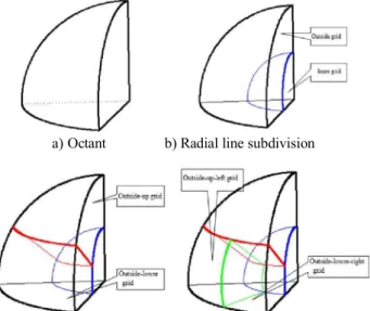
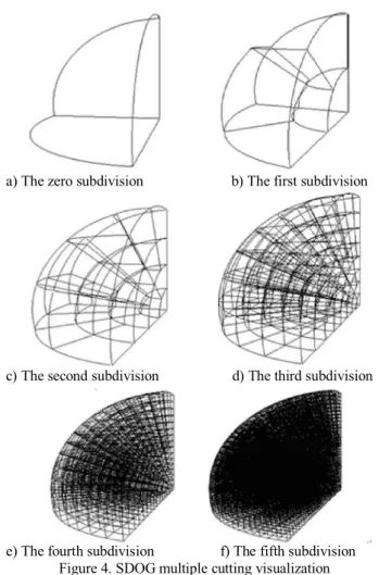
Neste trabalho o objetivo central foi a ampliação e adequação do procedimento e programa computacional baseado no programa comercial MSC.PATRAN, para a geração automática de modelos

Ousasse apontar algumas hipóteses para a solução desse problema público a partir do exposto dos autores usados como base para fundamentação teórica, da análise dos dados

Para tanto foi realizada uma pesquisa descritiva, utilizando-se da pesquisa documental, na Secretaria Nacional de Esporte de Alto Rendimento do Ministério do Esporte