ALONG THE LAST TWENTY FIVE YEARS (
)
SIDNEY ROSA VIEIRA (2*); SONIA CARMELA FALCI DECHEN (2)
ABSTRACT
Soil properties vary in space due to many causes. For this reason it is wise to know the magnitude and behaviour of the variability for adequate data analysis and decision making. Our work on spatial variability of soil properties in São
Paulo, Brazil began in 1982 with a very simple soil sampling in a small field. Much progress has been made since then on sampling designs, field equipment and methods, and mostly on computation equipment and softwares. This paper reports the results corresponding to some aspects of this progress, as far as the field, analysis and computation work are concerned. The objective of this study was to illustrate the use of geostatistics in data analysis for three sampling conditions on long term no-tillage system. The analysis is done on a wide range of field scales, variables, sampling
schemes as well as repeating sampling scheme for the same variable in different years. Semivariograms are compared for the same variables in different scales and sampling dates and depths as to provide a guide for sampling spacing and number of samples. Normalized crop yield parameters for many years are used in the discussion of time variability
and on the use of yield maps to locate management zones. The time of the year in which measurements of soil physical
properties are made affected the results both in terms of descriptive statistical and spatial dependence parameters. Crop
yields changed (soybean decrease and maize increase) with time of no-tillage but the real cause was not identified. The
length of time with no-tillage affected the range of dependence for the main crops (increased for soybean, maize and
oats) and therefore increased the size of the homogeneous management zones. The evolution of the sampling grid from
20 m with 63 sampling points to 10 m with 302 sampling points allowed for a much better knowledge of the spatial variability of crop yields but it had the reverse effect on the spatial variability of soil physical properties.
Key words: geostatistics, semivariogram, temporal variation, grain crop yield.
RESUMO
ESTUDOS DE VARIABILIDADE ESPACIAL EM SÃO PAULO, BRASIL AO LONGO DOS ÚLTIMOS VINTE E CINCO ANOS
Propriedades do solo variam no espaço devido a várias causas. Por esta razão, é importante sempre ter conhecimento da magnitude e do comportamento da variabilidade para uma análise adequada dos dados e auxiliar
na tomada de decisões. Trabalhos sobre variabilidade espacial de propriedades do solo em São Paulo se iniciaram em
1982, com uma amostragem bastante simples em uma pequena área. Desde aquela data, houve bastante progresso em amostragem, equipamentos e métodos de medição no campo e, principalmente, em equipamentos de computação e em programas especializados. Este trabalho relata os resultados relativos a alguns aspectos deste progresso no que concerne
a amostragens e medições no campo, análise e computação. O objetivo é ilustrar o uso da geoestatistica na análise de
dados para três condições de amostragem em um experimento de plantio direto de longa duração. A análise é feita em uma variedade de escalas de campo, variáveis, esquemas de amostragem bem como a repetição de amostragem de uma mesma variável em anos diferentes. Foram efetuadas comparações de semivariogramas e respectivos parâmetros para
uma determinada variável em escalas e amostragens diferentes com a intenção de ajudar na escolha de espaçamento e
número de amostras. Parâmetros de rendimento normalizado das culturas são usados nas discussões da variabilidade
temporal e no uso de mapas de rendimento para localizar zonas homogêneas de manejo. As épocas do ano nas quais as
propriedades físicas foram medidas afetaram os resultados tanto em termos de parâmetros de estatística descritiva como
de dependência espacial. O rendimento das culturas alterou (soja decresceu e milho aumentou) com o tempo de plantio direto, mas a causa desta alteração não foi identificada. O tempo com plantio direto afetou o alcance da dependência espacial para o rendimento das principais culturas (aumentou para soja, milho e aveia) e, portanto, causou aumento do tamanho de zonas homogêneas de manejo. A evolução da malha de amostragem de 20 m com 63 pontos para um malha
de 10 m com 302 pontos permitiu conhecimento mais detalhado da variabilidade espacial de rendimento de culturas, mas mostrou um efeito inverso na variabilidade espacial de propriedades físicas.
Palavras-chave: Geoestatistica, semivariograma, variação temporal, produtividade de grãos.
(1) Received for publication in September 9, 2008 and accepted in December 22, 2009.
1. INTRODUCTION
It is generally recognized that soils vary widely regarding their physical, chemical and biological nature. Parent materials and soil formation factors can vary due to their inherent characteristics and also due to conditions imposed by human actions. As consequence soil properties vary across a landscape in such a way as to reach equilibrium with the environmental conditions. The amount of variation over an area depends on many environmental conditions and how they acted on soil properties over time.
Spatial variability of soil properties has long been known to exist and has to be taken into account every time field sampling is performed. Beckettand WeBster (1971) presented a very comprehensive review with deep discussion of soil fertility variability. Soil variability can also occur as a result of cultivation, land use and erosion. salvianoet al. (1998) reported spatial variability in soil attributes as a result of land degradation due to erosion. There has been reports on spatial variability of soil properties, mostly affecting crop yield since the beginning of the 20th century (MontgoMery, 1913; Waynick, 1918; Harris, 1920), but a comprehensive tool to adequately analyse spatial variability was not available until 1971 (MatHeron, 1971). This tool, called geostatistics, contains a very important component called semivariogram which measures similarity between neighbouring observations. Semivariograms have been widely used in soil science for a number of physical (vieiraet al., 1981), chemical (Paz gonzálezet al., 2000) and biological (caMBardella et al., 1994) soil properties at a range of scales and with different grid sampling sizes. In the past, important contributions have been made to the discussion on general subjects such as optimal spacing of a regular grid for kriging interpolation (WeBster, 1985). In general most of the reports show that adequate evaluation of soil variability depends largely on the intensity of sampling design with respect to the size of the area under study. When a spatial structure pattern is not evidenced, it means that spatial variability within that particular sampling design is due to heterogeneity at a scale smaller than the distance between adjoining sampling points. If spatial dependence occurs, then using the semivariogram and by means of kriging interpolation method, values can be obtained optimally for the places not sampled and the corresponding kriging estimation variances can be computed (vieiraet al., 1983).
At the beginning of the last century there was a large concern on the effects of soil variability over field trials and experiments (Harris, 1920). The statistical knowledge available at that time recommended the use of classical statistical methods which requires that the variable under investigation be normally distributed and
spatially independent (snedecor and cocHran, 1967). As the field equipments and methods developed, the numerical knowledge of variability became increasingly evident and had to be somehow considered. Soil properties and crop yield components, instead of having random spatial distributions, have been reported to have spatial dependence, meaning that the observations are somehow related to their neighbours (vauclinet al., 1982; vieiraet al., 1983; Milleret al., 1988; souzaet al., 1997; Mulla, 1993). It seems obvious that the existence of spatial dependence is scale dependent. vieira (1997) found spatial dependence for soil fertility properties within an experimental plot of 30 by 30 m. On the other hand, the mean annual rainfall in the state of São Paulo, Brazil, showed spatial dependence up to 70 km (vieira and loMBardi neto, 1995). The assessment of spatial dependence requires the application of geostatistical procedures such as analysis of semivariograms (vieira, 2000) using kriging (vieiraet al., 1983; vieiraand loMBardi neto, 1995; vieira, 1997), cokriging (vauclin et al., 1983) and analysing maps produced with the interpolated values. Geostatistical techniques, including non-parametric models have been further developed in the last years, so that different algorithms producing different error of interpolation are now available (goovaerts, 1997). Nevertheless, ordinary kriging is still the most widely used interpolation method (vieira, 2000).
Long term experiments under tropical conditions using no-tillage are rare. Although it is known that the efficiency of the no-tillage system in conserving soil and water is climate dependent, it is still a very recommended management system mainly because it preserves the soil structure from one year to the next (castro et al., 2005). Therefore, there are reasons to believe that soil physical properties will tend to remain unchanged after the no-tillage system has been fully established, if the sampling and measuring tools are appropriate. On the other hand, changes in soil physical properties over time of no-tillage adoption may help the understanding of crop yield spatial distribution pattern not repeating over time. Moreover, besides affecting the soil water regime, the no-tillage system also requires unique fertilizer management as most of the fertilizer and liming is place at or close to the soil surface (Muzilli, 1981).
The objective of this study was to illustrate the use of geostatistics in the data analysis for three sampling conditions on long term no-tillage system.
2. MATERIAL AND METHODS
Study sites
are dominated by basic rocks (diabase). The soil is a clayey Latossolo Vermelho eutroférrico (eMBraPa, 2006) (Rhodic Eutrudox), located in a field of about 10% slope. Two fields were sampled for this study: 1. A 900 m2 field sampled in 1982 at 49 points located on a 5 m square grid as shown in figure 1a, where the X direction runs across the slope. This field was regularly cultivated with annual cereal crops with conventional tillage consisting of disk ploughing followed by a disk harrow; 2. A 3.42 ha field sampled in three different ways, according to figure 1b: a) from 1985 to 1995 the field was sampled at 63 points on a 20 m square grid; b) from 1996 to 2001 the field was sampled at 81 points on a 10 m square grid, and c) from 1997 to 2008 the field was sampled at 302 points on a 10 m square grid. Since 1985 this field is being cultivated with grain cereal crops under no-tillage. The two fields are located about 1000 m apart, at about 630 m above sea level, in a rolling topography with a slope range between 6% and 10%. The primary reasons for the selection of the site were the apparent natural variability as indicated by the spontaneous vegetation and the representation for other regions with the same soil type. The climate is subtropical with a mean annual rainfall of about 1500 mm, with 5-6 wet months (November to March) although variability may be rather large between years. The experimental area on the 3.42 ha field was regularly sampled every harvest time for the summer and winter crops in 2 x 2.5 m subplots, by cutting and weighing all mass above the soil. The cropping history of the site involves the use of no-tillage system on grain
crops, most of the time with two crops per year, for the last 23 years. Between 1965 and 1975 one third of the field (the left third part of the field on figure 1b) was used with grapes and the remaining two thirds with annual crops. The grapes were planted in rows with 3 m spacing, following the contour level. Afterwards the field was abandoned for another 10-year period, until 1985. Natural weed vegetation, mainly grasses, was grown after the field was left in fallow in 1975. In the first months of 1985 the field was first burnt out, cleared with bulldozer then moldboard plowed and disk harrowed and finally in April 1985 cultivated with Crotalaria juncea, without fertilizer addition or lime amendments. After the flowering of the Crotalaria juncea, 4000 kg ha-1 of lime was added while tilling the soil. Since then the field has been devoted to no-tillage annual crops.
Sampling and analysis
Soil sampling and field measurements
Field of 900 m2 - Soil samples were collected at each one of the 49 sampling points (Figure 1a) for soil texture analysis at the depths of 0-25 and 25-50 cm. Only clay content was analyzed in this work. One hundred cm3 core samples were collected at each one of the 49 sampling points (Figure 1a) at 0-10, 10-25 and 25-50 cm depth for soil bulk density determination and at 0-10 cm depth for porosity determination in the laboratory. This sampling took place on May 1982 and the analyses were performed according to caMargoet al. (1986).
Figure 1. Sampling lay out: (a) 900 m2 field with Clay content (g kg-1) for 0-25cm depth, sampled in 1982; (b) 3.42 ha field sampled
from 1985 to 2008 according to the legend in the map.
(a)
0 20 40 60 80 100 120 140 160 Direction X (m)
0 20 40 60 80 100 120 140 160 180 200
D
ir
e
c
ti
o
n
Y
(
m
)
1985 to 1995
2003 to 2008
1996 to 2002
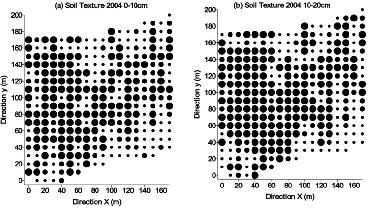
Field of 3.42 ha - Soil samples were taken from each one of the 63 sampling points (Figure 1b) at 0-25 cm depth for texture analysis in June 1985 and August 1988. Soil texture was performed using the pipette method for the clay and silt fractions, and sieving for 5 sand fractions according to caMargo et al. (1986). One hundred cm3 core samples were collected at each one of the 63 sampling points (Figure 1b) at the depths of 0-10 and 10-25 cm, for determination of, soil bulk density and soil porosity in the laboratory, in June 1985 and in August 1989. In April 2002, samples were collected at the depth of 0-10 cm on the 10 x 10 m grid shown in figure 1b, skipping two rows for each sampling in one direction so that the final sampling was then on a 30 m spacing in one direction and 10-m spacing on the other. Soil samples were collected on the 10 m square grid in April 2004 at the 10 cm depth. Soil cores were collected again at the 10 cm depth on the 302 points (Figure 1b) in March 2005. Saturated infiltration rate was measured on the 63 sampling points in 1990, on the 81 sampling points with 5 replicates on 1996 and in the 302 sampling points on September 2002, July 2003, September 2003 and July 2008 with the constant head field permeameter (vieira, 1998).
In figure 2, besides indicating the location where soil samples were collected for particle size analysis, the symbols used are proportional to the clay content to illustrate where the regions of high and low values are.
As it can be seen, the leftmost side of the field is almost completely filled with clay content values that yielded a classification of a very clayey soil (above 600 g kg-1).
Crop yield components
The crop yield components were measured in plots of 2 x 2.5 m, adjacent to the sampling points, measuring the final crop population, the total amount of straw and grain for each one of the crops. Crop yields were measured in 23 harvestings events as shown in Table 1.
In order to make comparisons between crop yields for different crops and different years, they were normalized to a dimensionless number, NYi, using
(
)
(
max min)
min
Y Y
Y Y
NY i
i = (1)
where Yi is the yield, Ymin and Ymax are, respectively, the minimum and maximum values for the yield. This relation was adapted from davis (1973).
Statistical methods
The statistical analysis used in this study involves an exploratory analysis with the examination of averages, coefficients of variation, extreme values and
Figure 2. Sampling lay out for the 3.42 ha field with texture at 0-10cm (a) and 10-20cm (b) sampled in 2004. 0 20 40 60 80 100 120 140 160
Direction X (m) 0
20 40 60 80 100 120 140 160 180 200
D
ir
e
c
ti
o
n
y
(
m
)
(a) Soil Texture 2004 0-10cm
0 20 40 60 80 100 120 140 160
Direction X (m) 0
20 40 60 80 100 120 140 160 180 200
D
ir
e
c
ti
o
n
y
(
m
)
normal distribution coefficients. The examination of the temporal evolution of descriptive statistical parameters over different sampling intensities may be useful to identify the adequate conditions for future work.
When data are sampled in such a way as to allow for the application of geostatistical analysis, the spatial dependence, according to vieira et al. (1983), can be evaluated by examining the semivariogram, which can be calculated using equation (2),
( ) (
)
[
]
=
+ )
(
1
2
h N
i
i i Z x h x
Z 2N(h)
1 =
(h) (2)
where N(h) is the number of pairs of values Z(xi), Z(xi+h) separated by a vector h. If the semivariogram increases with distance and stabilizes at the a priori variance value, it means that the variable under study is spatially correlated and all neighbours within the correlation range can be used to interpolate unknown values. Semivariograms may be scaled by dividing each semivariance value by a constant such as the square of the mean and the variance value, as suggested by vieira et al. (1997).
The calculation of the experimental semivariograms was carried out while checking for possible trends in the data sets. Omnidirectional
semivariograms were calculated using the program shown in vieira et al. (2002b). When semivariograms are calculated using equation (2), the result is a set of discrete values of distances along with the corresponding semivariances. Because any geostatistical calculation will require semivariances for any distance within the measured domain, there is a need to fit a mathematical model that would describe the variability. Semivariogram modeling is the foundation for geostatistical analysis, and can also be the most difficult and time consuming portion of the analysis. In part, this is due to the computationally intensive calculations, but it is also due to the difficulty in defining semivariogram models which reasonably honour the experimental semivariograms (McBratneyand WeBster, 1986).vieira (2000) describes the model fitting process and the cross validation of the fitted models. In this paper, the semivariograms used were fitted to either the spherical model
a h < 0 a h a
h C + C =
(h) 0 1
3
2 1 2
3
(3)
a > h C + C =
(h) 0 1
or the exponential model
d < h < 0 a h C
+ C =
(h) 0 1 1 exp 3 (4)
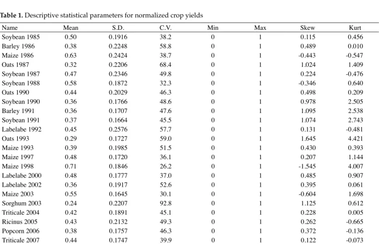
Table 1. Descriptive statistical parameters for normalized crop yields
Name Mean S.D. C.V. Min Max Skew Kurt
Soybean 1985 0.50 0.1916 38.2 0 1 0.115 0.456
Barley 1986 0.38 0.2248 58.8 0 1 0.489 0.010
Maize 1986 0.63 0.2424 38.7 0 1 -0.443 -0.547
Oats 1987 0.32 0.2206 68.4 0 1 1.024 1.409
Soybean 1987 0.47 0.2346 49.8 0 1 0.224 -0.476
Soybean 1988 0.58 0.1872 32.3 0 1 -0.346 0.640
Oats 1990 0.44 0.2029 46.3 0 1 0.498 0.209
Soybean 1990 0.36 0.1766 48.6 0 1 0.978 2.505
Barley 1991 0.36 0.1707 47.6 0 1 1.095 2.538
Soybean 1991 0.37 0.1664 45.5 0 1 1.074 2.743
Labelabe 1992 0.45 0.2576 57.7 0 1 0.131 -0.481
Oats 1993 0.29 0.1727 59.0 0 1 1.645 4.421
Maize 1993 0.39 0.1985 51.5 0 1 0.430 0.393
Maize 1997 0.48 0.1720 36.1 0 1 0.207 1.144
Maize 1998 0.71 0.1846 26.2 0 1 -1.545 4.007
Labelabe 2000 0.48 0.1777 37.0 0 1 0.485 0.907
Labelabe 2002 0.36 0.1917 52.6 0 1 0.395 0.061
Maize 2003 0.55 0.1645 30.1 0 1 -0.604 1.698
Sorghum 2003 0.24 0.2207 92.8 0 1 1.125 0.612
Triticale 2004 0.42 0.1891 45.1 0 1 0.228 0.005
Ricinus 2005 0.43 0.2132 49.3 0 1 0.262 -0.665
Popcorn 2006 0.38 0.1757 46.3 0 1 0.372 -0.136
where C0 is the nugget effect, C1 is the structural variance, a the range of spatial dependence and d is the maximum distance over the field. C0, C1 and a are the three parameters used in the semivariogram model fitting. Models were fit using least squares minimization and judgement of the coefficient of determination. Whenever there was any doubt on the parameters and model fitting, the jack knifing procedure was used to validate the model, according to vieira (2000).
caMBardella et al. (1994) proposed the calculation of a dependence degree (DD) expressed as a ratio between the nugget effect value (C0) and the sill (C0+C1) and classified as Weak if DD>75%, Moderate for 26%<DD<75%, and Strong for DD≤25%. ziMBack (2001) proposed a slight change on the calculation of the Dependence Degree (DD) as
(
0 1)
1001 + =
C C
C
DD (5)
which is classified as Weak if DD≤25%, Moderate if
26%<DD<75% and Strong if DD≥75%. Although these
two indexes are complementary the one proposed by ziMBack (2001) expresses better the dependence degree as the low numbers refer to weaker dependences and vice versa while the one proposed by caMBardella et al. (1994) is the reverse. For this reason, in this paper the dependence degree (DD) was calculated for all
semivariograms that showed spatial dependence according to ziMBack (2001).
The graphical representation of semivariogram parameters over time can reveal important changes in soil physical properties as a function of time of adoption of the using no-tillage system. This kind of analysis can help to understand the reasons why crop yield maps quite often do not repeat in time.
3. RESULTS AND DISCUSSION
The statistical parameters for the normalized yields of 23 crops are shown in table 1. In general mean yields are below 0.5, but most of time maize yields are the largest ones. Coefficients of variation (CV) for the winter crops (such as barley, oat and sorghum) are high (above 50%), due to irregular rainfall distribution. The triticale is an exception to this result with CV below 50% owing to its resistance to water shortage. It is noticeable the large variation for the same crop in different years, fact that makes it difficult to use yield maps for the delineation of management zones. Mulla (1993) reports on the problem of yield maps not repeating from one year to another for precision agriculture decisions.
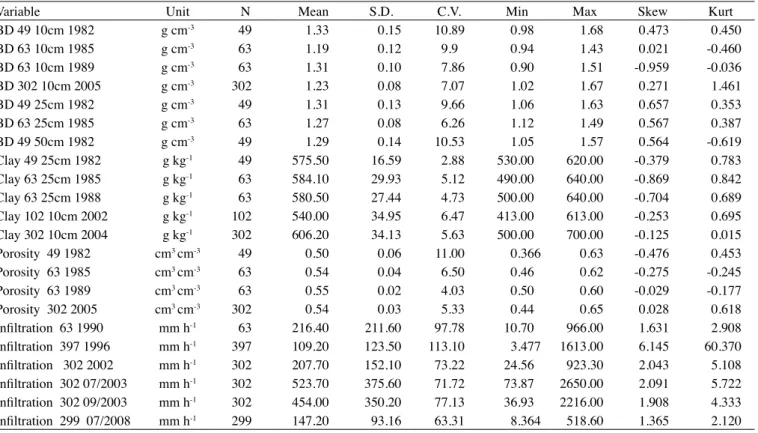
The descriptive statistical parameters for soil physical properties under study are shown in table 2. Except for the infiltration data, all other attributes approach normal distribution as the coefficients of
Table 2. Descriptive statistical parameters for soil properties analyzed
Variable Unit N Mean S.D. C.V. Min Max Skew Kurt
BD 49 10cm 1982 g cm-3 49 1.33 0.15 10.89 0.98 1.68 0.473 0.450
BD 63 10cm 1985 g cm-3 63 1.19 0.12 9.9 0.94 1.43 0.021 -0.460
BD 63 10cm 1989 g cm-3 63 1.31 0.10 7.86 0.90 1.51 -0.959 -0.036
BD 302 10cm 2005 g cm-3 302 1.23 0.08 7.07 1.02 1.67 0.271 1.461
BD 49 25cm 1982 g cm-3 49 1.31 0.13 9.66 1.06 1.63 0.657 0.353
BD 63 25cm 1985 g cm-3 63 1.27 0.08 6.26 1.12 1.49 0.567 0.387
BD 49 50cm 1982 g cm-3 49 1.29 0.14 10.53 1.05 1.57 0.564 -0.619
Clay 49 25cm 1982 g kg-1 49 575.50 16.59 2.88 530.00 620.00 -0.379 0.783
Clay 63 25cm 1985 g kg-1 63 584.10 29.93 5.12 490.00 640.00 -0.869 0.842
Clay 63 25cm 1988 g kg-1 63 580.50 27.44 4.73 500.00 640.00 -0.704 0.689
Clay 102 10cm 2002 g kg-1 102 540.00 34.95 6.47 413.00 613.00 -0.253 0.695
Clay 302 10cm 2004 g kg-1 302 606.20 34.13 5.63 500.00 700.00 -0.125 0.015
Porosity 49 1982 cm3 cm-3 49 0.50 0.06 11.00 0.366 0.63 -0.476 0.453
Porosity 63 1985 cm3 cm-3 63 0.54 0.04 6.50 0.46 0.62 -0.275 -0.245
Porosity 63 1989 cm3 cm-3 63 0.55 0.02 4.03 0.50 0.60 -0.029 -0.177
Porosity 302 2005 cm3 cm-3 302 0.54 0.03 5.33 0.44 0.65 0.028 0.618
Infiltration 63 1990 mm h-1 63 216.40 211.60 97.78 10.70 966.00 1.631 2.908
Infiltration 397 1996 mm h-1 397 109.20 123.50 113.10 3.477 1613.00 6.145 60.370
Infiltration 302 2002 mm h-1 302 207.70 152.10 73.22 24.56 923.30 2.043 5.108
Infiltration 302 07/2003 mm h-1 302 523.70 375.60 71.72 73.87 2650.00 2.091 5.722
Infiltration 302 09/2003 mm h-1 302 454.00 350.20 77.13 36.93 2216.00 1.908 4.333
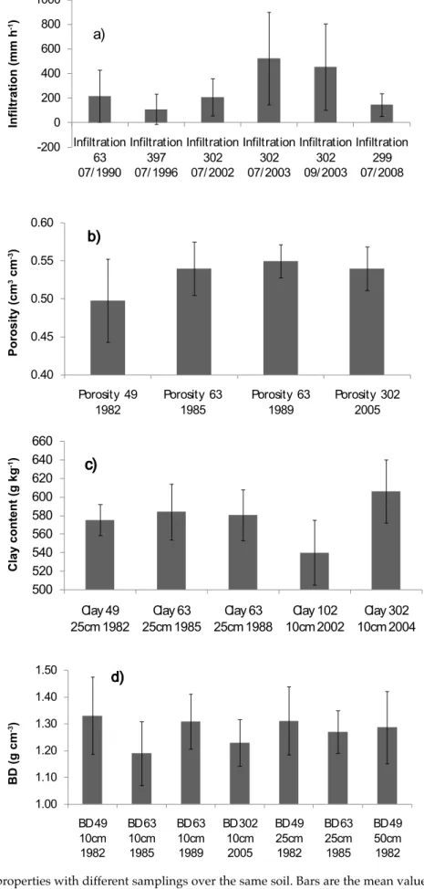
skewness and of kurtosis are very close to zero. These coefficients for the infiltration data indicate that they have a great number of small values and a few values really large as to make the distribution to approach a log normal. Infiltration rate values are very well known to have skewed distribution such as this (vieiraet al., 1981). All properties for which the number of values is 49 refer to the 900 m2 field. This field was only sampled once in 1982. The first seven lines show the results for bulk density (BD) over different sampling dates and depths. The range of variation of the mean BD values, within a minimum of 1.19 g cm-3 for values measured at the 3.42 ha field in 63 points in 1985 and a maximum of 1.33 g cm-3 for the 49 values sampled in the 900 m2 field in 1982, are not surprising for this type of soil under no-tillage. siqueira et al. (2008) found similar results using the clod method of measurement with three clod sizes. souzaet al. (1997) also found results within this range for an orange field. On the other hand, it was noticed that coefficients of variation (CV) for bulk density are all bellow 11%, which means that BD does not exhibit large changes even when different methods are used for the measurements. Taking the BD mean value measured in 1985 (1.19 g cm-3) as a reference and comparing with the value measured in 1989 (1.31 g cm-3) there was a 10% increase after 4 years of no-tillage. However, this trend did not continue as the value measured in 2005 decreased to 1.23 g cm-3 for the same depth and field. It should be emphasized that this value is the average of 302 samples over a much wider spatial distribution (Figure 1b), and therefore, represents very well this attribute for this particular condition. vieira et al. (2002a), working on no-tillage on this same type of soil under another condition found bulk density values within the above range and found high correlation with soil porosity.
The range of variation for the mean values for clay content (from 540 to 606.2 g kg-1) shown in table 2 are not very easily explained since these samples come all from the same soil with only different sampling strategies. One possible explanation for these differences is the laboratory method as the sampling made on 2002 in 102 points was analyzed using the pipette method while the others were all analyzed using the soil hydrometer method. According to caMargo et al. (1986) the soil hydrometer method tends to over estimate the clay content for soils situated in the clayey texture class or above. On the other hand, the coefficients of variation for clay content are all very low (below 7%) indicating that the variation of this attribute on the studied field is small.
The porosity results are within usual values reported in the literature (vieiraet al., 2002a; siqueiraet al. 2008) with very low coefficients of variation (CV) and
approaching a normal distribution for all the sampling dates analyzed.
The infiltration rate was measured in all different dates in the same field (3.42 ha), using the same method (vieira, 1998) varying the number of samples (63, 397, 302 and 299), the sampling grid (20-m grid for the 63 samples, 10 m grid in the 81 sampling points with five replications for the 397, 10-m grid for 302 samples, where the last one had 3 missing values). However, one factor that may have been significant is the month at which the sampling took place both because of the cracks developed in this soil in the dry season (May to September) and also, and very important the crop present at the time of sampling. The means of the sampling made in 07/2003 and in 09/2003 are large because of the effect of cracks but also because it was right after two grass crops (Maize in the summer and Sorghum in the winter season). The grass crop root system seems to have a major effect on soil infiltration rate and so does soil structure cracks (vieiraet al. 1988). The infiltration measured in 1990 (216.4 mm h-1) under soybean crop, the one in 1996 (109.2 mm h-1) under fallow and the one measured in 2002 (207.7 mm h-1) under labelabe (leguminous crop) were all performed in January. Obviously the leguminous crop root system does not have the same effect over infiltration as the grass crops.
Figure 3. Soil physical properties with different samplings over the same soil. Bars are the mean values of 49, 63 or 302 samples
± one standard error.
-200 0 200 400 600 800 1000
Infiltration 63 07/ 1990
Infiltration 397 07/ 1996
Infiltration 302 07/ 2002
Infiltration 302 07/ 2003
Infiltration 302 09/ 2003
Infiltration 299 07/ 2008 a)
0.40 0.45 0.50 0.55 0.60
Porosity 49 1982
Porosity 63 1985
Porosity 63 1989
Porosity 302 2005 b)
500 520 540 560 580 600 620 640 660
Clay 49 25cm 1982
Clay 63 25cm 1985
Clay 63 25cm 1988
Clay 102 10cm 2002
Clay 302 10cm 2004
c)
1.00 1.10 1.20 1.30 1.40 1.50
BD 49 10cm 1982
BD 63 10cm 1985
BD 63 10cm 1989
BD 302 10cm 2005
BD 49 25cm 1982
BD 63 25cm 1985
BD 49 50cm 1982 d)
BD (g cm
-3)
Clay content (g kg
-1)
Porosity (cm
3 cm -3)
Infiltration (mm h
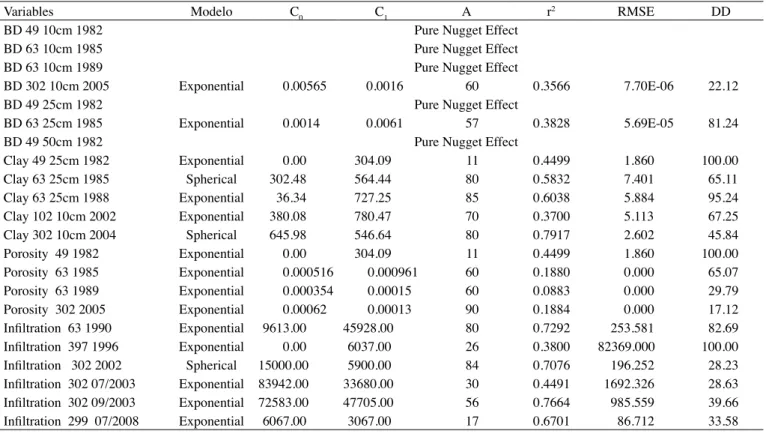
Table 3. Parameters of the models fitted to the semivariograms of soil variables
Variables Modelo C0 C1 A r2 RMSE DD
BD 49 10cm 1982 Pure Nugget Effect
BD 63 10cm 1985 Pure Nugget Effect
BD 63 10cm 1989 Pure Nugget Effect
BD 302 10cm 2005 Exponential 0.00565 0.0016 60 0.3566 7.70E-06 22.12
BD 49 25cm 1982 Pure Nugget Effect
BD 63 25cm 1985 Exponential 0.0014 0.0061 57 0.3828 5.69E-05 81.24
BD 49 50cm 1982 Pure Nugget Effect
Clay 49 25cm 1982 Exponential 0.00 304.09 11 0.4499 1.860 100.00
Clay 63 25cm 1985 Spherical 302.48 564.44 80 0.5832 7.401 65.11
Clay 63 25cm 1988 Exponential 36.34 727.25 85 0.6038 5.884 95.24
Clay 102 10cm 2002 Exponential 380.08 780.47 70 0.3700 5.113 67.25
Clay 302 10cm 2004 Spherical 645.98 546.64 80 0.7917 2.602 45.84
Porosity 49 1982 Exponential 0.00 304.09 11 0.4499 1.860 100.00
Porosity 63 1985 Exponential 0.000516 0.000961 60 0.1880 0.000 65.07
Porosity 63 1989 Exponential 0.000354 0.00015 60 0.0883 0.000 29.79
Porosity 302 2005 Exponential 0.00062 0.00013 90 0.1884 0.000 17.12
Infiltration 63 1990 Exponential 9613.00 45928.00 80 0.7292 253.581 82.69
Infiltration 397 1996 Exponential 0.00 6037.00 26 0.3800 82369.000 100.00
Infiltration 302 2002 Spherical 15000.00 5900.00 84 0.7076 196.252 28.23
Infiltration 302 07/2003 Exponential 83942.00 33680.00 30 0.4491 1692.326 28.63
Infiltration 302 09/2003 Exponential 72583.00 47705.00 56 0.7664 985.559 39.66
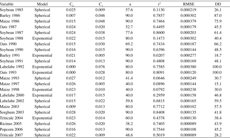
Infiltration 299 07/2008 Exponential 6067.00 3067.00 17 0.6701 86.712 33.58 Tables 3 and 4 show the parameters for the models
fitted to semivariograms for the soil physical properties and for the normalized yield data of 45 semivariograms, five showed pure nugget effects, nineteen were fitted with exponential models and twenty one with spherical. McBratney and WeBster (1986) pointed out that the spherical model is the one that occurs for most situations. All five pure nugget effect semivariograms are for bulk density because this attribute has a very small variability and low coefficients of variation. This also means that the fields sampled do not have regions of compaction problems and the bulk density values are randomly distributed over the areas. The dependence degree values calculated according to ziMBack (2001) (last column in tables 3 and 4) are in general high, indicating enough spatial dependence in order to use kriging interpolation. vieira (2000) recommends that kriging interpolation will not have any advantage to other interpolation procedures if the dependence degree is below 10%. The smallest dependence degree values are for infiltration, a variable that has a very high random variation owing to its nature of being dependent of many other variables such as root and worm canals and soil cracks (vieiraet al., 1981). The range of spatial dependence found for most variables indicates that the present sampling strategy with 302 sampling points on a 10 m square grid is enough for most geostatistical evaluations in this field.
The temporal evolution of the dependence degree for clay content, porosity and infiltration, and of the range of spatial dependence for infiltration are shown in figure 4. For all the variables, in general, there was a decrease in the above parameters with the time with no-tillage. The most noticeable of this is the decrease in the dependence degree for porosity (Figure 4b) reaching a value just below 20% for the 2005 sampling. It is possible that this value is also reaching a stable situation with the time of no-tillage, developing soil structure. It is also noticeable the decrease in dependence degree for clay content (Figure 4c). grego and vieira (2005) found spatial dependence for clay content in a small experimental plot.
Table 4. Parameters of the models fitted to the semivariograms of normalized yield data
Variable Model C0 C1 a r2 RMSE DD
Soybean 1985 Spherical 0.025 0.009 57.6 0.1130 0.000219 26.1
Barley 1986 Spherical 0.007 0.046 90.0 0.7857 0.000302 87.0
Maize 1986 Spherical 0.015 0.048 90.0 0.7464 0.000379 75.9
Oats 1987 Spherical 0.024 0.020 52.7 0.4495 0.000179 45.5
Soybean 1987 Spherical 0.024 0.038 77.6 0.8600 0.000203 61.4
Soybean 1988 Exponential 0.022 0.015 80.0 0.1473 0.000302 40.4
Oats 1990 Spherical 0.015 0.030 69.2 0.7434 0.000187 66.2
Soybean 1990 Spherical 0.016 0.015 90.0 0.6396 0.000144 48.5
Barley 1991 Exponential 0.021 0.005 90.0 0.0207 0.000277 18.7
Soybean 1991 Spherical 0.014 0.013 90.0 0.4808 0.000169 48.1
Labelabe 1992 Exponential 0.000 0.076 80.0 0.7585 0.000380 100.0
Oats 1993 Exponential 0.000 0.028 80.0 0.8091 0.000120 100.0
Maize 1993 Spherical 0.027 0.012 41.4 0.0646 0.000249 30.7
Maize 1997 Spherical 0.026 0.005 40.0 0.0896 0.000144 15.1
Maize 1998 Exponential 0.023 0.010 40.0 0.0792 0.000238 30.0
Labelabe 2000 Exponential 0.017 0.015 40.0 0.2959 0.000158 46.8
Labelabe 2002 Spherical 0.015 0.022 59.8 0.6815 0.000165 59.5
Maize 2003 Spherical 0.009 0.013 80.0 0.7712 0.000102 57.5
Sorghum 2003 Spherical 0.028 0.020 90.0 0.8408 0.000135 41.8
Triticale 2004 Exponential 0.023 0.014 60.0 0.4378 0.000130 38.4
Ricinus 2005 Spherical 0.026 0.020 38.2 0.7405 0.000089 43.9
Popcorn 2006 Spherical 0.016 0.013 90.0 0.7544 0.000108 45.2
Triticale 2007 Spherical 0.022 0.009 48.6 0.5019 0.000089 28.2
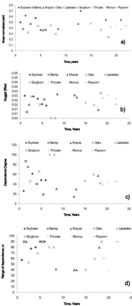
the nugget effect values drastically decreased. There was an increase in dependence degree for soybean and oat values (Figure 5c) and an initial decrease for maize up to about 12 years of no-tillage with a slight increase again after this time. A general look at figure 5c indicates that there was a decrease in the dependence degree with time of no-tillage regardless the kind of crop. The range of dependence does not seem to have a clear trend with the time of no-tillage, except that it showed a pronounced increase for soybean and oat. From figure 5b-d it can be said that management zones for most crops have increased in size with the time of no-tillage. In particular for maize there was an initial decrease until about 10 years (Figure 5b-d) followed by an increase after that time. It should be remembered that after 10 years of no-tillage (1995) there was a change in sampling spacing from 20 m square grid to 10 m square grid. That means that the shorter spacing improved the assessment of the spatial variability for crop yields and allowed for enough information in order to suggest some management zone establishing in the field.
Long term and frequently monitored no-tillage experiments are rare mostly within tropical conditions. vieira et al. (2002a) report on some changes in soil physical properties under no-tillage and crop rotation and concluded that both bulk density and saturated
hydraulic conductivity are significantly affected by the changes in organic matter content. carvalHoet al. (2002) investigated the effect of soil tillage on the spatial variability of soil chemical properties and concluded that no-tillage promoted significant increase in organic matter content
4. CONCLUSIONS
1. The time of the year in which measurements of soil physical properties are made affected the results both in terms of descriptive statistical and spatial dependence parameters.
2. Crop yields changed (soybean decrease and maize increase) with time of no-tillage but the real cause was not identified.
3. The length of time with no-tillage affected the range of dependence for the main crops (increased for soybean, maize and oats) and therefore increased the size of the homogeneous management zones.
Figure 4. Temporal evolution of semivariogram parameters for soil physical properties.
0 20 40 60 80 100 120
Infiltration 63 1990
Infiltration 397 1996
Infiltration 302 2002
Infiltration 302 07/ 2003
Infiltration 302 09/ 2003
Infiltration 299 07/ 2008
D
e
p
e
n
d
e
n
ce
D
e
g
re
e
a)
0 20 40 60 80 100 120
Porosity 49 1982 Porosity 63 1985 Porosity 63 1989 Porosity 302 2005
D
e
p
e
n
d
e
n
ce
d
e
g
re
e
b)
0 20 40 60 80 100 120
Clay 49 25cm 1982Clay 63 25cm 1985Clay 63 25cm 1988 Clay 102 10cm 2002
Clay 302 10cm 2004
D
e
p
e
n
d
e
n
ce
D
e
g
re
e
c)
0 10 20 30 40 50 60 70 80 90
Infiltration 63 1990
Infiltration 397 1996
Infiltration 302 2002
Infiltration 302 07/ 2003
Infiltration 302 09/ 2003
Infiltration 299 07/ 2008
R
a
n
g
e
o
f d
e
p
e
n
d
e
n
ce
Figure 5. Temporal evolution of normalized yield and the corresponding semivariogram parameters.
0 0.1 0.2 0.3 0.4 0.5 0.6 0.7 0.8
0 5 10 15 20
M
e
an
n
o
rm
al
iz
e
d
y
ie
ld
Time, years
a)
Soybean Barley Mayze Oats Labelabe Sorghum Triticale Ricinus Popcorn
0.00 0.01 0.01 0.02 0.02 0.03 0.03 0.04 0.04 0.05 0.05
0 5 10 15 20 25
N
u
gg
e
t
Ef
fe
ct
Time, Years
b)
Soybean Barley Mayze Oats LabelabeSorghum Triticale Ricinus Popcorn
0 20 40 60 80 100 120
0 5 10 15 20 25
D
e
p
e
n
d
e
n
ce
D
e
g
re
e
Time, Years
c)
Soybean Barley Mayze Oats LabelabeSorghum Triticale Ricinus Popcorn
0 10 20 30 40 50 60 70 80 90 100
0 5 10 15 20 25
R
a
n
g
e
o
f
d
e
p
e
n
d
e
n
ce
, m
Time, Years
d)
Soybean Barley Mayze Oats LabelabeREFERENCES
BECKETT, P.H.T.; WEBSTER, R. Soil variability: a review. Soil Fertility, v.34, p.1-15, 1971.
CAMARGO, O.A.; MONIZ, A.C; JORGE, J.A.; VALADARES, J.M.A.S. Métodos de análise química, mineralógica e física de solos do Instituto Agronômico de Campinas. Campinas: Instituto Agronômico, 1986. 94p. (Boletim técnico, 106)
CARVALHO, J.R.P.; SILVEIRA, P.M.; VIEIRA, S.R. Geoestatística na determinação da variabilidade espacial de características químicas do solo sob diferentes preparos. Pesquisa Agropecuária Brasileira, v.37, p.1151-1159, 2002.
CASTRO, O. M., MBAGWU, J. S. C., VIEIRA, S. R., KANTHACK, R., DECHEN, S. C. F., DE MARIA, I. C.,
BRAGA, N. R. Effect of no-tillage crop rotation systems on nutrient status of a rhodic ferralsol in southern Brazil. Agro-Science Journal of Tropical Agriculture, Food, Environment and Extension, v.4, p.8 - 14, 2005.
CAMBARDELLA, C. A.; MOORMAN, T. B.; NOVAK J. M.; PARKIN T. B.; KARLEN, D. L.; TURCO, R. F.; KONOPKA, A.
E. Field scale variability of soil properties in central Iowa soils. Soil Science Society America Journal, Madison, v. 58, n. 5, p. 1501-1511, 1994..
DAVIS, J.C. Statistics and data analysis in geology. John Wiley, New York, 1973. 550p.
EMPRESA BRASILEIRA DE PESQUISA
AGROPECUÁRIA-EMBRAPA. Centro Nacional de Pesquisa de Solos. Sistema
Brasileiro de Classificação de Solos. 2.ed. Rio de Janeiro, 2006. 306p.
GOOVAERTS, P. Geostatistics for natural resources evaluation. New York: Oxford University Press, 1997. 500p. (Applied Geostatistics Series)
GREGO, C.R.; VIEIRA, S.R. Variabilidade espacial de propiedades físicas do solo em uma parcela experimental. Revista Brasileira de Ciência do Solo, v.29, p.169-177, 2005.
HARRIS, J.A. Practical universality of field heterogeneity as a factor influencing plot yields. Journal of Agricultural Research, v. 19, p. 279-314, 1920.
MATHERON, G. The theory of regionalized variables and its application. Fontainebleau: Les Cahiers du Centre de Morphologie Mathematique, Fontainebleau, 1971. 56 p. (Fascicule 5)
McBRATNEY, A. B.; WEBSTER, R. Choosing functions for semi-variograms of soil properties and fitting them to sampling
estimates. Journal of Soil Science, v.37, p.617-639, 1986.
MILLER, M.P.; SINGER, M.J.; NIELSEN, D.R. Spatial variability of wheat yield and soil properties on complex hills. Soil Science Society of America Journal, v.52, p.1133-1141, 1988.
MONTGOMERY, E.G. Experiments in wheat breeding: experimental error in the nursery and variation in nitrogen and yield. Washington: United States Department of Agriculture/ Bureau of Plant Industry, 1913. p.5-61. (USDA Bulletin, 269) MULLA, D.J. Mapping and managing spatial patterns in soil fertility and crop yield. In: Soil specific crop management. Madison: Soil Science Society of America, 1993. p.15-26.
MUZILLI, O. O. Manejo da Fertilidade do Solo, In: IAPAR. Plantio Direto no Estado do Paraná. Londrina: IAPAR, 1981. p.43-58 (Circular nº 23)
PAZ GONZÁLEZ, A.; VIEIRA, S.R.; TABOADA CASTRO, M.T. The effect of cultivation on the spatial variability of
selected properties of an umbric horizon. Geoderma, v.97, p 273-292, 2000.
SALVIANO, A.A.C.; VIEIRA, S.R.; SPAROVEK, G. Variabilidade espacial de atributos de solo e de Crotalaria juncea (L.) em área severamente erodida. Revista Brasileira de Ciência do Solo, v. 22, p.115-122, 1998.
SIQUEIRA, G.M.; VIEIRA, S.R.; CEDDIA, M.B. variabilidade
de atributos físicos do solo determinados por métodos diversos. Bragantia, v.67, p.693-699, 2008.
SNEDECOR, G.W.; COCHRAN, W.G. Statistical methods. 6th
Edition. Ames, Iowa: State University Press, 1967. 593p. SOUZA, L. S.; COGO, N.P.; VIEIRA, S.R. Variabilidade de
propriedades físicas e químicas do solo em um pomar cítrico. Revista Brasileira de Ciência do Solo, v. 21, p. 367-372, 1997.
VAUCLIN, M.; VIEIRA, S.R.; BERNARD, R.; HATFIELD,
J.L. Spatial variability of two transects of a bare soil. Water Resources Research, v.18, p.1677-1686, 1982.
VAUCLIN, M.; VIEIRA, S.R.; VACHAUD, G.; NIELSEN, D.R. The use of cokriging with limited field soil observations. Soil Science Society of America Journal, v.47, p.175-184, 1983.
VIEIRA, S.R. Permeâmetro: novo aliado na avaliação de
manejo do solo. O Agronômico, v.47-50, p.32-33, 1998.
VIEIRA, S.R. Uso de geoestatística em estudos de variabilidade
espacial de propriedades do solo. In: NOVAIS, R.F. (Ed.). Tópicos em Ciência do Solo. Viçosa: Sociedade Brasileira de Ciência do Solo, 2000. p.1-54.
VIEIRA, S.R. Variabilidade espacial de argila, silte e atributos químicos em uma parcela experimental em um Latossolo Roxo de Campinas (SP). Bragantia, v.57, p.181-190, 1997.
VIEIRA, S.R.; HATFIELD, J.L.; NIELSEN, D.R.; BIGGAR, J.W.
Geostatistical theory and application to variability of some agronomical properties. Hilgardia, v.51, p.1-75, 1983.
VIEIRA, S.R.; LOMBARDI NETO, F. Variabilidade espacial
VIEIRA, S.R.; MBAGWU, J.S.C.; CASTRO, O.M.; ALVES, M.C.;
DECHEN, S.C.F.; DE MARIA, I.C. Changes in some physical properties of a typic haplorthox in southern Brazil under no-tillage crop rotation systems. Agro-Science Journal of Agriculture, Food, Environment and Extension, v.3, p.1-12, 2002a.
VIEIRA, S.R.; MILLETE, J.; TOPP, G.C.; REYNOLDS, W.D.
Handbook for geostatistical analysis of variability in soil and climate data. In: ALVAREZ V., V.H.; SCHAEFER, C.E.G.R.;
BARROS, N.F.; MELLO, J.W.V.; COSTA, L.M., (Ed.). Tópicos em ciência do solo. Viçosa. Sociedade Brasileira de Ciência do Solo, 2002b. v.2, p.1-45.
VIEIRA, S.R.; NIELSEN, D.R.; BIGGAR, J.W. Spatial variability
of field-measured infiltration rate. Soil Science Society of America Journal, v.45, p.1040-1048, 1981.
VIEIRA, S.R.; NIELSEN, D.R.; BIGGAR, J.W.; TILLOTSON, P.M. The scaling of semivariograms and the kriging estimation. Revista Brasileira de Ciência do Solo, v. 21, p.525-533, 1997.
VIEIRA, S.R.; REYNOLDS, W.D.; TOPP, G.C. Spatial
variability of hydraulic properties in a highly structured
clay soil. In: WIERENGA, P.J.; BACHELET, D. (Eds.). Validation of flow and transport models for the unsaturated zone, 1988, Las Cruces. Proceedings… Las Cruces: Department of Agronomy and Horticulture, New
Mexico State University, 1988. p. 471-483 (Research Report
88—SS-04)
WAYNICK, D.D. Variability in soils and its significance to past and future soil investigations. I. Statistical study of nitrification
in soils. Agricultural Sciences, v.3, p.243-270, 1918.
WEBSTER, R. Quantitative spatial analysis of soil in field. Advances in Soil Science, v.3, p.2-56, 1985.
ZIMBACK, C.R.L. Analise espacial de atributos químicos de
solos para fins de mapeamento da fertilidade do solo. 2001.