André Quintão de Almeida(1), Rodolfo Marcondes Silva Souza(2), Diego Campana Loureiro(1), Donizete dos Reis Pereira(3), Marcus Aurélio Soares Cruz(4) and Jodnes Sobreira Vieira(5)
(1)Universidade Federal de Sergipe (UFS), Departamento de Engenharia Agrícola, Campus São Cristovão, Cidade Universitária
Prof. José Aloísio de Campos, Avenida Marechal Rondon, s/no, Jardim Rosa Elze, CEP 49100-000 São Cristóvão, SE, Brazil. E-mail:
[email protected], [email protected] (2)Universidade Federal de Pernambuco, Departamento de Energia Nuclear, Avenida
Prof. Luiz Freire, no 1.000, Cidade Universitária, CEP 50740-545 Recife, PE, Brazil. E-mail: [email protected] (3)Universidade
Federal de Viçosa, Campus Florestal, Rodovia LMG 818, Km 6, CEP 35690-000 Florestal, MG, Brazil. E-mail: [email protected]
(4)Embrapa Tabuleiros Costeiros, Núcleo de Apoio à Programação, Avenida Beira Mar, no 3.250, Jardins, CEP 49025-040 Aracaju, SE,
Brazil. E-mail: [email protected] (5)UFS, Departamento de Zootecnia, Campus São Cristovão, Cidade Universitária Prof. José
Aloísio de Campos, Avenida Marechal Rondon, s/no, Jardim Rosa Elze, CEP 49100-000 São Cristóvão, SE, Brazil. E-mail: [email protected]
Abstract – The objective of this work was to model the spatial dependence and to map the rainfall erosivity index (EI30) in the semiarid region of Brazil. Registers of monthly erosivity from 210 rainfall stations were used, with daily time series equal to or greater than 15 years. Based on the values of the EI30, a spatial dependence model was made by adjusting the semivariogram. From the semivariogram models, erosivity isoline maps were generated with a kriging interpolator. According to the historical data series, the maximum monthly average value of the EI30 was observed in March, and the annual value ranged from 1,439 to 5,864 MJ mm ha-1 per year, classified as low and moderate, respectively. The highest EI
30 values were obtained in the northern and southern extremes of the semiarid region. Average spatial dependence was observed for rainfall erosivity, in most months, especially with the spherical semivariogram model. The range of erosivity varied from 62 to 1,508 km for the monthly EI30 and was of approximately 1,046 km for the annual one. The applied model, with the validation of the semivariograms using the jackknife test, allows the spatialization of the EI30 for the semiarid region of Brazil.
Index terms: EI30, geostatistics, Northeastern Brazil, semivariogram.
Modelagem da dependência espacial do índice de
erosividade das chuvas no semiárido brasileiro
Resumo – O objetivo deste trabalho foi modelar a dependência espacial e mapear o índice de erosividade das chuvas (EI30) na região semiárida do Brasil. Foram utilizados registros de erosividade mensal de 210 postos pluviométricos, com série temporal diária igual ou superior a 15 anos. Com base nos valores do EI30, a modelagem da dependência espacial foi realizada pelo ajuste do semivariograma. A partir dos modelos de semivariograma, foram gerados mapas de isolinhas de erosividade com interpolador da krigagem. De acordo com a série histórica de dados, o valor máximo mensal médio do EI30 foi observado em março, e o valor anual variou de 1.439 a 5.864 MJ mm ha-1 por ano, classificado como baixo e moderado, respectivamente. Os maiores valores do EI30 foram obtidos nos extremos norte e sul da região semiárida. Foi observada dependência espacial média para erosividade da chuva, para a maioria dos meses, principalmente com o modelo de semivariograma esférico. O alcance da erosividade variou entre 62 e 1.508 km, para o EI30 mensal, e foi de, aproximadamente, 1.046 km para o anual. A modelagem aplicada, com a validação dos semivariogramas pelo teste de jackknife, permite a espacialização do EI30 para a região semiárida do Brasil.
Termos para indexação: EI30, geoestatística, Nordeste, semivariograma.
Introduction
Brazil, due to its size, is affected by different climate types. According to official data from Ministério da Integração Nacional, the Brazilian
semiarid is located in most of the Northeastern region of the country and covers an area of 969,589 km2 (Brasil, 2005). The semiarid climate
concentrated in a few months of the year; average air temperatures between 23 and 27°C; low relative humidity values; and potential evapotranspiration of approximately 2,000 mm per year (Moscati & Gan, 2007; Hastenrath, 2012). However, the various atmospheric circulation systems in the region make climatology complex, resulting in great climatic variability, mainly in relation to rainfall, with precipitation events that vary in time and space.
The characterization of rainfall in a certain region is an important tool for soil management and conservation (Silva et al., 2010). This is because, in the erosive process, the factor erosivity reflects the capacity of rainfall to erode the soil in an area with no cover, which is directly related to the duration, intensity, and frequency of precipitation events (Montebeller et al., 2007; Peñalva Bazzano et al., 2010; Mello et al., 2012).
The factor rainfall erosivity is one of the main parameters entered into the universal soil loss equation (USLE) proposed by Wischmeier & Smith (1978) and can be expressed by indexes that are based on the physical characteristics of local rainfall. The erosivity index (EI30) is the most commonly used for
Brazilian conditions, since it is considered the most suitable for intertropical reality, and represents the result of the kinetic energy of a raindrop when it reaches the soil by its maximum intensity (Mello et al., 2015).
Determining EI30 values during the year allows
identifying the months when the risks of soil and water losses are higher (Silva et al., 2010). In addition, understanding the pattern of the spatial distribution of erosivity is important for planning and managing water resources, as well as for establishing priority areas and times of the year for soil and water conservation and management.
Studies on the spatial dependence of rainfall erosivity were developed for some regions of Brazil (Mello et al., 2007, 2008; Silva et al., 2010). Mello et al. (2012), for example, modeled the spatial dependence of the monthly and annual EI30 for the
entire state of Espírito Santo, and found a high degree of spatial dependence. Silva et al. (2010), in turn, adjusted geostatistical models using rainfall data for the southeastern region of the state of Minas Gerais, for fast-growing tree farming. The results
obtained in these studies are indicative that the EI30 values show a wide range and degree of spatial
dependence.
However, in general, studies on rainfall erosivity in Northeastern Brazil are not very common (Oliveira et al., 2013), among which stands out the one carried out by Cantalice et al. (2009). The apparent lack of interest in the EI30 in this region
might be related to the shortage of historical rainfall records older than 20 years, in short-time intervals (less than 10 min), which are needed to calculate the EI30. Regarding spatial dependence, the number of
studies in Northeastern Brazil is even more limited, especially in the semiarid region. Recently, some studies on rainfall erosivity were conducted, but for the entire country. Mello et al. (2013) adjusted multiple models to calculate rainfall erosivity for the whole country, according to geographic coordinates, whereas Mello et al. (2015) assessed the performance of different interpolation methods, including kriging, to spatialize EI30 values for the
Brazilian territory.
The objective of this work was to model the spatial dependence and to map the EI30 in the semiarid
region of Brazil.
Materials and Methods
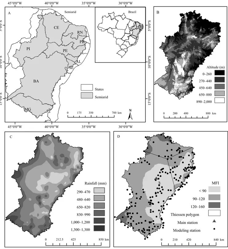
The study was carried out using data from the semiarid region of Brazil (Figure 1 A), which has an area of 969,589 km2, including parts of nine Brazilian
states (Brasil, 2005): Alagoas, Bahia, Ceará, Minas Gerais, Paraíba, Pernambuco, Piauí, Rio Grande do Norte, and Sergipe. The approximate population is of 22 million inhabitants, which represents 11.8% of the country’s population, according to Instituto Brasileiro de Geografia e Estatística (IBGE, 2010). The terrain of the region is varied, with altitudes ranging from 0 to 2,000 m, mainly in the central region (Figure 1 B). The average annual rainfall ranges between 290 and 1,300 mm per year (Figure 1 C).
the stations (codes 1036063 and 124102) with the smallest monitoring interval had data from 15 years, from 10/1/1991 to 12/1/2006. Of the 210 stations, 42
neighbored the study area and were used to improve the interpolation process. The errors found in the daily records were corrected by the inverse distance
Figure 1. Location map of the Brazilian semiarid region (A), altitude map (B), rainfall map (C), and annual map of the
weighting method (Di Luzio et al., 2008), based on the three closest stations.
Three main equations were used to calculate the monthly EI30, according to the modified
Fournier index (MFI). The first equation was obtained by Silva (2004), and the second and third ones by Cantalice et al. (2009), as follows:
EI p Pa
EI p Pa
EI
i i
i i
i 30
2 0 7387
30
2 0 58
30 73 989 61 81 95 =
(
)
=(
)
= . ; . ; . . . 448 2 0 56 pi Pa
(
)
. ;in which EI30i is the erosivity index of the average
monthly rainfall (MJ mm ha-1 per month); p
i is the
historical rainfall (mm) for month i, based on the daily series equal to or greater than 15 years; and Pa is the historical annual rainfall (mm). The annual erosivity value (EI30) was calculated by adding
the monthly values from each rainfall station. These equations were used to estimate the monthly erosivity of the 210 rainfall stations used for modelling, by considering the similarity of each station with the area of the Thiessen polygon for each main station (Figure 1 D).
The MFI reflects the potential of rainfall to erode the soil of a certain region and was estimated for each of the 210 stations by the equation:
MFI p Pa i i = =
∑
2 1 12Afterwards, a map of the MFI was created by using the inverse distance weighted interpolation method for the entire semiarid region (Figure 1 D). Consequently, it was possible to identify the spatial distribution of this index throughout the area, as well as the location of the main stations, according to this distribution.
The EI30i and EI30 values were evaluated by the
average, maximum, and minimum values; the standard deviation; and the coefficient of variation (CV). Variability was classified according to the CV values (Pimentel-Gomes & Garcia, 2002), as: low, CV <10%; medium, 10%< CV <20%; high, 20%< CV <30%; and very high, CV >30%. The data normality hypothesis was evaluated by the Kolmogorov-Smirnov test.
Spatial dependence was analyzed by geostatistical techniques, using adjusted semivariograms. The
semivariance function was calculated for all directions (isotropic semivariogram), in order to observe the spatial dependence of the data. Previously, the following theoretical models of semivariograms were adjusted: spherical, exponential, and Gaussian.
The choice of the best adjustment was made by validating the semivariograms after running the jackknife test (Vieira et al., 2010), which analyzes the consistency of the data calculated by the kriging interpolator, based on the adjusted (experimental) semivariograms. The estimate is considered adequate when the average (µjk) and the variance (σjk) of the
reduced error are close to 0 and 1, respectively. The semivariogram was adjusted by the weighted least squares method, using the R 3.2.2 software (R Core Team, 2015) and the geoR package (Ribeiro Jr. & Diggle, 2001).
The degree of spatial dependence (DSD) was calculated based on the percent relationship between the nugget effect (C0) and the sill, given
by the sum of C0 and the structured variation (C)
[DSD = C/(C0 + C)100]. The DSD was classified as:
low, DSD <25%; medium, 25%≤ DSD ≤75%; and strong, DSD >75% (Robertson, 1998).
Results and Discussion
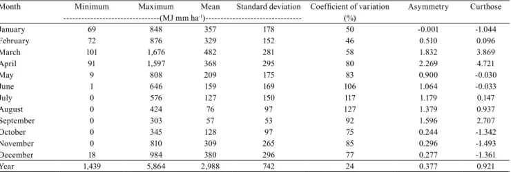
The highest EI30i values (1,676 MJ mm ha-1 per
month) were observed in March, and the lowest ones from June to November (Table 1), with greatest variation in the period between December and May, when soil and water conservation and management practices in the region must be intensified. The greatest standard deviation in the data was obtained in December and the smallest one in September, which showed the greatest rate of generalized drought throughout the semiarid region; it should be noted that although this month had a low average erosivity index (57 MJ mm ha-1), this value might be enough to
cause soil loss, depending on other factors.
spatial dependence analysis. Moreover, the CVs for the EI30 for the semiarid region were high, which can
be justified, given the fact that the region is strongly affected by different rainfall patterns (Moscati & Gan, 2007; Hastenrath, 2012; Rodriguez et al., 2015).
The annual minimum, maximum, and average values for the EI30 were 1,439, 5,865, and 2,988 MJ
mm ha-1 per year, respectively, which can be classified
as being of medium potential. These results were similar to those reported by Mello et al. (2013) in the Northeastern region of Brazil, when adjusting
several models to estimate rainfall erosivity for the whole country.
All months presented spatial dependence (Table 2). The spherical semivariogram model performed best for modelling spatial dependence between January and September. In October, due to the abrupt change in the EI30, the exponential model
showed better results. In November and December, the Gaussian model provided the best adjustments for the semivariograms. Although the application of the exponential model is more commonly accepted
Table 1. Descriptive statistics of the rainfall erosivity index in the semiarid region of Brazil, based on daily rainfall series equal to or greater than 15 years of data.
Month Minimum Maximum Mean Standard deviation Coefficient of variation Asymmetry Curthose
---(MJ mm ha-1)--- (%)
January 69 848 357 178 50 -0.001 -1.044
February 72 876 329 152 46 0.510 0.096
March 101 1,676 482 281 58 1.832 3.869
April 91 1,597 368 295 80 2.269 4.721
May 9 808 209 175 83 0.900 -0.030
June 1 646 159 169 106 1.064 -0.033
July 0 576 127 150 117 1.179 0.147
August 0 424 76 97 127 1.379 0.937
September 0 303 57 53 92 1.596 2.707
October 0 345 128 97 75 0.244 -1.342
November 0 810 309 265 85 0.296 -1.493
December 18 984 380 296 77 0.277 -1.361
Year 1,439 5,864 2,988 742 24 0.377 0.921
Table 2. Estimates of the semivariograms adjusted for the monthly and annual rainfall (MJ mm ha-1) values for the semiarid region of Brazil, calculated from daily series equal to or greater than 15 years of data.
Month Model C0 C DSD (%) A (km) µjk σjk
January Spherical 11,750 42,597 21.62 1,508 -0.0004 0.9020
February Spherical 14,312 12,165 54.05 914 0.0006 0.9404
March Spherical 24,268 57,360 29.73 789 0.0002 0.9884
April Spherical 7,856 72,194 9.81 831 -0.0001 1.0245
May Spherical 4,738 24,484 16.22 762 0.0061 1.1357
June Spherical 14,282 14,282 50.00 700 0.0021 0.9207
July Spherical 10,213 12,128 45.71 439 0.0040 0.9942
August Spherical 4,448 5,560 44.44 431 0.0042 0.9626
September Spherical 823 2,044 28.70 308 0.0054 0.9669
October Exponential 480 1,222 28.23 62 0.0023 1.4465
November Gaussian 2,814 52,067 5.13 614 0.0006 1.3759
December Gaussian 6,936 513,281 1.33 1,038 -0.0005 1.6684
Total Spherical 154,158 617,702 19.97 1,046 0.0044 0.9961
(Mello et al., 2007, 2008, 2012; Montebeller et al., 2007), the spherical (more frequently) and the Gaussian models showed the best results in the present study. While studying the modelling and continuity of the EI30 in eastern Minas Gerais, Silva
et al. (2010) also found better results with Gaussian models.
The parameters obtained from the theoretical semivariograms (C0, C, range, and DSD) showed
different classes of variability during the year in the semiarid region (Table 2). Overall, C0 increased
linearly with average erosivity, which shows that the absolute error in the sampling was greater during the rainy months. According to Burgos et al. (2006), the C0 is directly related to the sampling error, to
short-range or to unexplained variability. The relationship with average erosivity may be an indicative of the need for a greater number of meteorological stations in order to reduce this error, especially during the rainy season. In 7 of the 12 months, erosivity presented a medium degree of spatial dependence and, in the rest of them, a low one.
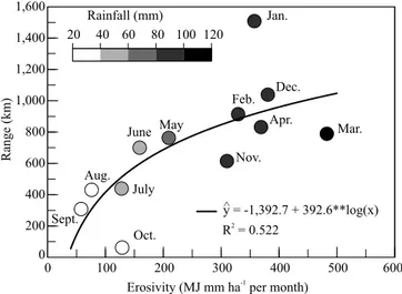
The range is an important parameter of the semivariogram that has practical interpretations, since it shows the distance between two points that have spatial dependence. Samplings separated
by a distance lower than the range are spatially correlated, whereas those separated by a greater distance are independent (Wang et al., 2015). The range of erosivity varied from 62.18 km in October to 1,508 km in January (Table 2). The temporal variability of rainfall significantly (p<0.01) affected the range of erosivity, which was represented by a logarithmic regression (Figure 2). It is possible to observe two clusters, which corresponded to the rainy season, from November to April, and to the dry season, from May to October.
In the months with rainfall above 60 mm, the average erosivity was greater than 300 MJ mm ha-1
per month, and the range in this season was of at least 600 km. The low range during the dry season in the semiarid region indicates that the rainfall events in this season were isolated.
As observed in the semivariograms, it was possible to note the effect of the monthly seasonality of erosivity in the region (Figure 3). The erosivity values started to increase in October, starting in the state of Minas Gerais and in the south of Bahia. Over the months, these values increased significantly in the northern direction of the semiarid region. The highest values were observed in March and April, concentrated in the states of Ceará, Piauí, and Maranhão; and the lowest ones were recorded in September. In the fifth month of the year, rainfall erosivity started to decrease, following the same direction, from the south to the north of the semiarid region.
When considering the annual values for the EI30,
a variation between 1,757 and 4,870 MJ mm ha-1
per year was observed, which allowed classifying the semiarid region as having a weak erosive potential. However, this does not mean that water and soil conservation and management practices and techniques do not have to be applied in areas with low erosive potential (Figure 4 A and B). While analyzing the annual spatial variability of rainfall erosivity in the state of Rio de Janeiro, Montebeller et al. (2007) found values between 2,000 and 6,000 MJ mm ha-1 per year for the northern region of the state.
In the northern region of the state of Espírito Santo, Mello et al. (2007) also obtained low annual erosivity values associated with lower rainfall.
Jan. Feb. Mar. Apr.
May June July Aug.
Sept. Oct. Nov. Dec.
Latitude
Longitude
1,800
1,620
1,440
1,260
1,080
900
720
540
360
180
0
MJ mm ha
per month
-1
Figure 3. Spatial distribution of monthly mean erosivity in the semiarid region of Brazil. Daily series equal to or greater than 15 years of data.
Conclusions
1. The rainfall erosivity index in the semiarid region of Brazil shows a medium degree of spatial dependence from February to March and from June to October, and a low degree in the other months.
2. The spherical model is the most appropriate to represent the spatial distribution of erosivity and is better adjusted to the dry season, whereas the Gaussian model better represents the rainy season.
3. The applied models allow estimating the annual and monthly erosivity values, and the spatialization of the semiarid region of Brazil.
Acknowledgments
To Agência Nacional de Águas (ANA), for the availability of the rainfall data; to Fundação de Amparo à Ciência e Tecnologia de Pernambuco (Facepe) and to Coordenação de Aperfeiçoamento de Pessoal de Nível Superior (Capes, process No. 88887.136369/2017-00), for financial support.
References
ANA. Agência Nacional de Águas (Brasil). HidroWeb: sistemas
de informações hidrológicas. Available at: <http://hidroweb.ana. gov.br>. Accessed on: Mar. 10 2015.
BRASIL. Secretaria de Políticas de Desenvolvimento Regional. Nova delimitação do semi-árido brasileiro.
[2005]. Available at: ˂http://www.mi.gov.br/c/document_ l i b r a r y/g e t _ f i l e? u u i d = 0 a a 2 b 9 b5 - a a 4 d - 4 b55 - a 6 e1-82faf0762763&groupId=24915˃. Accessed on: May 12 2015.
BURGOS, P.; MADEJÓN, E.; PÉREZ-DE-MORA, A.; CABRERA, F. Spatial variability of the chemical characteristics of a trace-element-contaminated soil before and after remediation. Geoderma, v.130, p.157-175, 2006. DOI: 10.1016/j. geoderma.2005.01.016.
CANTALICE, J.R.B.; BEZERRA, S.A.; FIGUEIRA, S.B.; INÁCIO, E. dos S.B.; SILVA, M.D.R. de O. Linhas isoerosivas do estado de Pernambuco – 1ª aproximação. Revista Caatinga, v.22, p.75-80, 2009.
DI LUZIO, M.; JOHNSON, G.L.; DALY, C.; EISCHEID, J.K.; ARNOLD, J.G. Constructing retrospective gridded daily precipitation and temperature datasets for the conterminous United States. Journal of Applied Meteorology and Climatology, v.47, p.475-497, 2008. DOI: 10.1175/2007JAMC1356.1.
DIGGLE, P.J.; RIBEIRO JR., P.J. Model-based geostatistics. London: Springer, 2007. 230p.
HASTENRATH, S. Exploring the climate problems of Brazil’s Nordeste: a review. Climatic Change, v.112, p.243-251, 2012. DOI: 10.1007/s10584-011-0227-1.
IBGE. Instituto Brasileiro de Geografia e Estatística. Censo
demográfico 2010. 2010. Available at: ˂http://www.sidra.ibge.
gov.br/bda/tabela/listabl.asp?z=cd&o=5&i=P&c=761˃. Accessed
on: May 5 2015.
MELLO, C.R. de; SÁ, M.A.C. de; CURI, N.; MELLO, J.M. de;
VIOLA, M.R.; SILVA, A.M. da. Erosividade mensal e anual
da chuva no Estado de Minas Gerais. Pesquisa Agropecuária
Brasileira, v.42, p.537-545, 2007. DOI:
10.1590/S0100-204X2007000400012.
MELLO, C.R. de; VIOLA, M.R.; CURI, N.; SILVA, A.M. da.
Distribuição espacial da precipitação e da erosividade da chuva mensal e anual no Estado do Espírito Santo.Revista Brasileira
de Ciência do Solo, v.36, p.1878-1891, 2012. DOI:
10.1590/S0100-06832012000600022.
MELLO, C.R. de; VIOLA, M.R.; MELLO, J.M. de; SILVA, A.M.
da. Continuidade espacial de chuvas intensas no Estado de Minas Gerais. Ciência e Agrotecnologia, v.32, p.532-539, 2008. DOI: 10.1590/S1413-70542008000200029.
MELLO, C.R. de; VIOLA, M.R.; OWENS, P.R.; MELLO,
J.M. de; BESKOW, S. Interpolation methods for improving the RUSLE R-factor mapping in Brazil. Journal of Soil and Water
Conservation,v.70, p.182-197, 2015. DOI: 10.2489/jswc.70.3.182.
MELLO, C.R.; VIOLA, M.R.; BESKOW, S.; NORTON, L.D. Multivariate models for annual rainfall erosivity in Brazil. Geoderma, v.202/203, p.88-102, 2013. DOI: 10.1016/j. geoderma.2013.03.009.
MONTEBELLER, C.A.; CEDDIA, M.B.; CARVALHO, D.F. de; VIEIRA, S.R.; FRANCO, E.M. Variabilidade espacial
do potencial erosivo das chuvas no Estado do Rio de Janeiro.
Engenharia Agrícola, v.27, p.426-435, 2007. DOI: 10.1590/
S0100-69162007000300011.
MOSCATI, M.C. de L.; GAN, M.A. Rainfall variability in the rainy season of semi-arid zone of Northeast Brazil (NEB) and its relation to wind regime. International Journal of Climatology, v.27, p.493-512, 2007. DOI: 10.1002/joc.1408.
OLIVEIRA, P.T.S.; WENDLAND, E.; NEARING, M.A. Rainfall
erosivity in Brazil: a review. Catena, v.100, p.139-147, 2013. DOI: 10.1016/j.catena.2012.08.006.
PEÑALVA BAZZANO, M.G.; ELTZ, F.L.F; CASSOL, E.A.
Erosividade e características hidrológicas das chuvas de Rio Grande (RS). Revista Brasileira de Ciência do Solo, v.34, p.235-244, 2010. DOI: 10.1590/S0100-06832010000100024.
PIMENTEL-GOMES, F.; GARCIA, C.H. Estatística aplicada
a experimentos agronômicos e florestais: exposição com exemplos e orientações para uso de aplicativos. São Paulo: Fealq, 2002. 309p.
R CORE TEAM. R: A language and environment for statistical
computing. Vienna: R Foundation for Statistical Computing, 2015. Available at: <http://www.R-project.org/>. Accessed on:
Sept. 6 2016.
ROBERTSON, G.P. GS+ geostatistics for the environmental
sciences: GS+ user’s guide. Plainwell: Gamma Design Software,
1998. 152p.
RODRIGUEZ, R.D.G.; SINGH, V.P.; PRUSKI, F.F.;
CALEGARIO, A.T. Using entropy theory to improve the
definition of homogeneous regions in the semi-arid region of
Brazil. Hydrological Sciences Journal, v.61, p.2096-2109, 2015. DOI: 10.1080/02626667.2015.1083651.
SILVA, A.M. da. Rainfall erosivity map for Brazil. Catena, v.57,
p.251-259, 2004. DOI: 10.1016/j.catena.2003.11.006.
SILVA, M.A. da; SILVA, M.L.N.; CURI, N.; SANTOS, G.R.
dos; MARQUES, J.J.G. de S. e M.; MENEZES, M.D. de; LEITE,
F.P. Avaliação e espacialização da erosividade da chuva no Vale
do Rio Doce, região Centro-Leste do Estado de Minas Gerais.
Revista Brasileira de Ciência do Solo, v.34, p.1029-1039, 2010.
DOI: 10.1590/S0100-06832010000400003.
VIEIRA, S.R.; CARVALHO, J.R.P. de; PAZ GONZÁLEZ, A.
Jack knifing for semivariogram validation. Bragantia, v.69,
p.97-105, 2010. Supplement. DOI: 10.1590/S0006-87052010000500011. WANG, J.; YANG, R.; BAI, Z. Spatial variability and sampling optimization of soil organic carbon and total nitrogen for Minesoils of the Loess Plateau using geostatistics. Ecological Engineering, v.82, p.159-164, 2015. DOI: 10.1016/j.ecoleng.2015.04.103. WISCHMEIER, W.H.; SMITH, D.D. Predicting rainfall erosion
losses: a guide to conservation planning. Washington: USDA,
1978. 58p.