Analog Computers and Recursive Functions Over
the Reals
Daniel Silva Gra¸ca
CLC and ADM/FCT, Universidade do Algarve, C. Gambelas,
8000-062 Faro, Portugal
Jos´e F´elix Costa
DM/IST, Universidade T´ecnica de Lisboa, Av. Rovisco Pais,
1049-001 Lisboa, Portugal
March 14, 2003
Abstract
In this paper we show that Shannon’s General Purpose Analog Com-puter (GPAC) is equivalent to a particular class of recursive functions over the reals with the flavour of Kleene’s classical recursive function theory.
We first consider the GPAC and several of its extensions to show that all these models have drawbacks and we introduce an alternative continuous-time model of computation that solves these problems. We also show that this new model preserves all the significant relations involv-ing the previous models (namely, the equivalence with the differentially algebraic functions).
We then continue with the topic of recursive functions over the reals, and we show full connections between functions generated by the model introduced so far and a particular class of recursive functions over the reals.
1
Introduction
Digital computation has been, since the thirties, the most important compu-tational model, mainly due to the unifying work of Turing. Turing clarified the notion of algorithm, giving it a precise meaning, and introduced a coherent framework for discrete computation.
Nevertheless, computers need not be digital. In fact, the first computers were analog computers. In an analog computer, the internal states are continu-ous, rather than discrete as in digital computation. The first analog computers were especially well suited to solve ordinary differential equations and were ef-fectively used to solve many military and civilian problems during World War II
(e.g. gunfire control) and in the fifties and sixties (e.g. aircraft design). Unfor-tunately, because of the nonexistence of a coherent theoretical basis for analog computation and the fact that analog computing technology almost didn’t im-prove when compared with its digital counterpart in the last half century, analog computation was about to be forgotten with the emergence of digital computa-tion.
Despite this period of oblivion, analog computation is again regaining in-terest. The search for new models that could provide an adequate notion of computation and complexity for the dynamical systems that are currently used to model the physical world contributed to change the situation. However, rel-atively little work exists on a general theory of analog computation, and this still seems far away.
In this paper we will go to the roots of analog computation by recalling Shannon’s General Purpose Analog Computer (GPAC) [14]. We will point out some problems that appear in the scope of this model and also in its subsequent versions. We will then present an alternative model (the feedforward GPAC: FF-GPAC) that solves the problems referred to for the GPAC. We will also show that the FF-GPAC model is more robust than the GPAC, but still preserves the fundamental properties (equivalence with differentially algebraic functions).
Our objective is to develop some of the ideas presented in the seminal paper [11]. In this paper, Moore introduced a recursion theory over the reals and proved some results establishing links with classical recursion theory and also with the GPAC. Unfortunately, these results presented some gaps and, hence, the primary goal of our work is precisely to provide an adequate framework to obtain, wherever possible, similar results to those presented by Moore. In particular, we are interested in the connections between recursive functions over the reals and functions generated by the GPAC. While working on this topic we have found some further problems not referred to in the existing literature (at least to our knowledge) and a major revision of the GPAC was needed for our purposes.
2
The GPAC model
In 1941, Shannon introduced the General Purpose Analog Computer [14] as a mathematical model of an analog device, the Differential Analyzer [1]. This model basically consists of circuits composed of (a finite number of) “black boxes” as indicated in fig. 2.1 (the so-called analog units).1
It is required that two inputs and two outputs can never be interconnected. It is also required that each input is connected to, at most, one output.
The GPAC model has been mainly applied to functions depending on one variable. In this case, we say that a unary function y is generated by a GPAC
U on some interval I ⊆ R if we can prescribe some initial conditions to the
1For reasons of simplicity, we will usually identify objects with functions. The context will
be enough to decide which is the case. For instance, in figure 2.1,Rtot u(x)dv(x) should be
integrators of U at x = a ∈ I such that if x is applied to every input that is not connected to an output, then y equals the output of some unit for values of x in
I. For functions of more than one variable we may easily adapt this definition.
We will assume that if we have more than one distinct input for a GPAC, then they all depend on a parameter t that we will call the time (this is not very clear in existing literature. Shannon [14] assumes independent variables as inputs. Pour-El [13] talks on inputs depending on the time, but then assumes independent variables). For the one variable case, these approaches are equiva-lent: if x is the input of a GPAC, simply take x as the independent variable.
×k ku
u
A constant multiplier unit associated to the real value k
+ v u u+v An adder unit R v u Rt t0u(x)dv(x) An integrator unit 1 1
A constant function unit Figure 2.1: Representations of different types of units in a GPAC.
Definition 1 A unary function y is differentially algebraic (d.a.) on some set
I if there exists some natural number n (where n > 0) and some (n + 2)-ary nonzero polynomial P with real coefficients such that
P (x, y(x), ..., y(n)(x)) = 0,
for every x ∈ I.2
In what follows, we will assume that I ⊆ R is a closed, bounded interval with non-empty interior.
In his paper [14], Shannon presented an argument for the following fact: Claim 2 A unary function can be generated by a GPAC if and only if the
function is differentially algebraic.
This result indicates that a large class of functions, such as polynomials, trigonometric functions, elliptic functions, etc., could actually be generated by a GPAC. As a corollary some functions such as the Gamma function,
Γ(x) = Z ∞
0
tx−1e−tdt,
cannot be generated because they are not d.a. functions (cf. [2, pp. 49,50]).
2Note that this definition of differential algebraic function does not imply a definite degree
Unfortunately, the original proof of claim 2 has some gaps, as indicated on pp. 13-14 of [13]. In this paper, Pour-El was also concerned with showing some relations in the spirit of claim 2. In order to achieve this result, she introduced an alternative definition for the GPAC based on differential equations, that we will call the theoretic GPAC (T-GPAC: this is not the usual notation, but we use it in order to distinguish this model from Shannon’s GPAC). In essence, y is generated by a T-GPAC if there is some system of differential equations
A(x, y)dy
dx = b(x, y),
where y = (y1, ..., yn), such that A(x, y) and b(x, y) are n×n and n×1 matrices,
respectively, with linear entries and, moreover, y is one of the yi’s. The original
paper [13] can be referred for more details on the T-GPAC. Pour-El proved (with some corrections made by Lipshitz and Rubel in [9]) the following results: Theorem 3 (Pour-El) Let y be a differentially algebraic function on I. Then
there exists a closed subinterval I0 ⊆ I with non-empty interior such that, on
I0, y can be generated by a T-GPAC.
Theorem 4 (Pour-El, Lipshitz, Rubel) If y is generable on I by a T-GPAC,
then there is a closed subinterval I0 ⊆ I with non-empty interior such that, on
I0, y is differentially algebraic.
Although the model presented by Pour-El is apparently different from Shan-non’s GPAC, Pour-El presented the following result:
Claim 5 If a function y is generated on I by a GPAC, it is generated on I by
a T-GPAC.
This claim is the main reason why people referring to the GPAC actually recall Pour-El’s definition, instead of Shannon’s GPAC. Therefore the T-GPAC could be seen as a model that extends the GPAC, being able to compute func-tions generated by a Differential Analyzer. However, the original proof of claim 5 [13, proposition 1] has some gaps.3
Hence we will not deal with the T-GPAC because we don’t have known relationships between functions generated by this model and functions generated by some existing analog computers (the Differential Analyzer).
We could therefore turn to Shannon’s GPAC, but this model itself presents some problems. Besides the problem indicated with claim 2, we also have to deal with some more subtle details.
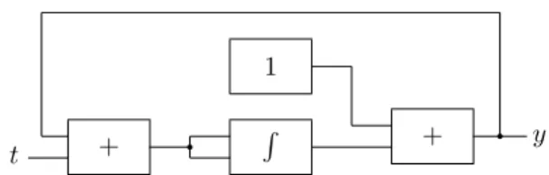
Consider the GPAC indicated in fig. 2.2.
3(We assume that the reader is referring to [13] for details) In that proposition she, in
fact, presents an argument where she states that if y is generated by a GPAC, then there exist functions (y2, ..., yn) satisfying the equation of condition 1 and condition 2 of definition
10. But she never shows that (y2, ..., yn) is the unique solution of that equation and she also
does not show condition 3. She only gives a physical argument to condition 3 on p. 12 when defining domain of generation, but does not give any formal proof.
+ q R
t +
1
q y Figure 2.2: A circuit that admits two distinct solutions as outputs. It is not difficult to see that y at time t is given by
y(t) = 1 +
Z t
0
(y(x) + x)d(y(x) + x).
We are supposing that t0= 0 and that the initial output of the integrator is 0.
When we start the computation, we get two possible solutions:
y±(t) = 1 ±
√
−2t − t.
Therefore, we cannot have a physical implementation of this circuit (in partic-ular, there is no Differential Analyzer that simulates this circuit). This is very problematic. We will solve this problem in the next section.
3
The FF-GPAC model
In this section, we will introduce a new model based on Shannon’s GPAC (it is a particular form of it), the FF-GPAC, that does not have the problems indicated in the previous section for the GPAC. In particular, we will be able to show that the output of each unit is unique on some “maximal interval” and that the relations indicated in theorems 3 and 4 will remain valid if we substitute the T-GPAC by the FF-GPAC model.
We had occasion to see that the output of a unit in a GPAC can be non-unique. We believe that this is due to the lack of restrictions on the GPAC, that allows connections with arbitrary feedback. Of course, feedback is desirable since, without it, we would get an uninteresting model. However, we believe that too much feedback can be harmful. In particular, we believe that this is the cause for the abnormal behavior of circuit 2.2. So, in this new model, we will restrict the feedback allowed.
Let us first give a brief overview of the standard procedure used to deal with the GPAC (with one input corresponding to the independent variable x). We can consider that every output of a GPAC is the output of an integrator. In fact, suppose that the output y is the output of some unit Ak. Hence, we may
introduce a new integrator and connect the input associated to the variable of integration to the output of Ak, and the input associated to the integrand to
a constant function unit. If we set the initial condition of the output of the integrator to be y(t0), the output of this integrator will be precisely y.
Proceeding in a similar way as in [14] (or [13]), let U be a GPAC with n − 1 integrators U2, ..., Un, having as outputs y2, ..., yn, respectively. Let y0= 1 and
let y1 = x. Then, each input of an integrator must be the output of one of
the following: an adder, an integrator, a constant function unit, or a constant multiplier. Hence, the integrand of Uk can be expressed as
Pn
i=0akiyi and the
variable of integration asPni=0bkiyi, for some suitable constants aki, bki. Thus,
the output of Uk, yk, can be expressed as
yk= Z x x0 n X i=0 akiyid n X j=0 bkjyj + ck, or yk= Z x x0 n X i,j=0 akibkjyidyj+ ck.
We may simplify the last expression by taking ck
ij= akibkj. It follows that y0 k = n X i,j=0 ck ijyiy0j, k = 2, ..., n. (1)
Hence, we could assert that it is equivalent to say that y is generated by a GPAC (in the sense that it is a solution for a system of equations where each equation is associated to a unit) and that y is a solution of some system of differential equations with the particular structure of (1). Although this seems a clear and natural procedure, we believe that we have to be more careful with it. For instance, why should we consider that the inputs of the integrator Uk could be
expressed asPni=0akiyi and
Pn
i=0bkiyi for some constants aki, bkj? We could
have as input the output of a circuit like the one of fig. 3.1.
+
1 q
Figure 3.1: A circuit that admits no solutions as outputs.
This circuit follows the definition of a GPAC, but we cannot say that its output is a linear combination of the input, because it does not exist (the output of the circuit is a solution of the equation x = x + 1). However these circuits are admissible in Shannon’s or Pour-El’s frameworks. But we would like to keep relations as in (1). To do so, we introduce the concept of linear circuit as follows. Definition 6 A linear circuit is an acyclic GPAC built only with adders,
con-stant multipliers, and concon-stant function units in the following inductive way: 1. A constant function unit is a linear circuit with zero inputs and one output; 2. A constant multiplier is a linear circuit with one input and one output;
3. An adder is a linear circuit with two inputs and one output;
4. If A is a linear circuit and if we connect the output of A to a constant multiplier, the resulting GPAC is a linear circuit. It has as inputs the inputs of A and as outputs, the output of the constant multiplier;
5. If A and B are linear circuits and if we connect the outputs of A and B to an adder, then the resulting circuit is a linear circuit in which the inputs are the inputs of A and B, and the output is the output of the adder.
The proof of the following proposition will be left to the reader.
Theorem 7 If x1, ..., xn are the inputs of a linear circuit, then the output of
the circuit will be y = c0+ c1x1+ ... + cnxn, where c0, c1, ..., cn are appropriate
constants. Reciprocally, if y = c0+c1x1+...+cnxn, then there is a linear circuit
with inputs x1, ..., xn, and output y.
We next introduce a new type of unit.
• Input unit: A zero-input, one-output unit.
The input units may be considered as interface units for the inputs from outside world in order that they can be used by a GPAC (although we may pick an output directly from the GPAC).
We now present the main definition of this section.
Definition 8 Consider a GPAC U with n integrators U1, ..., Un. Suppose that
to each integrator Ui, i = 1, ..., n, we can associate two linear circuits, Aiand Bi,
with the property that the integrand and the variable of integration inputs of Ui
are connected to the outputs of Ai and Bi, respectively. Suppose also that each
input of the linear circuits Ai and Bi is connected to one of the following: the
output of an integrator or to an input unit. U is said to be a feedforward GPAC (FF-GPAC) iff there exists an enumeration of the integrators of U, U1, ..., Un,
such that the variable of integration of the kth integrator can be expressed as ck+ m X i=1 ckixi+ k−1 X i=1 ¯ckiyi, for all k = 1, ..., n, (2)
(see fig. 3.2) where yi is the output of Ui, for i = 1, ..., n, xj is the input
associated to the jth input unit, and ck, ckj, ¯cki are suitable constants, for all
k = 1, ..., n, j = 1, ..., m, and i = 1, ..., k − 1.
Note that in a FF-GPAC we can link the output of Uk directly to the input of
Ur (as long as (2) is satisfied) because this is equivalent to having a constant
R
L(1,x1,...,xm,y1,...,yk−1)
L(1,x1,...,xm,y1,...,yn) y k
Figure 3.2: Schema of the inputs and outputs of Ukin the
FF-GPAC U. L(z1, ..., zr) denotes a linear combination (with real
coefficients) of z1, ..., zr.
We can also have a notion of function generated by a FF-GPAC using a straightforward adaptation of the corresponding definition for the case of the GPAC. We can also suppose that each function generated by a FF-GPAC is the output of an integrator.
Before continuing with our work, we have to set up more conditions on this model. We have admitted that the inputs x1, ..., xm of a GPAC are functions
of a parameter t, but we didn’t make any assumption on these functions (about computability, differentiability, or whatever). When we consider the integrator units, one problem still arises: if I = [a, b] is a closed interval, the Riemann-Stieltjes integralRIϕ(t)dψ(t) is not defined for every pair of functions ϕ, ψ, even
if they are continuous [16].
However, it is possible to show that if ϕ, ψ are continuously differentiable on I, then RIϕ(x)dψ(x) is defined. So, from now on, we will always assume
that the inputs are continuously differentiable functions of the time. And if the outputs of all units are defined for all t ∈ I, where I is an interval, then we will also assume that they are continuous in that interval. This is needed for the following results and may be seen as physical constraints to which all units are subjected.
4
Properties of the FF-GPAC
We now state the following theorems. Their proofs can be found in the disser-tation [6].
Theorem 9 Suppose that the input functions of a FF-GPAC are of class Cr
on some interval I, for some r ≥ 1, possibly ∞. Then the outputs are also of class Cron I.
Theorem 10 Consider a FF-GPAC with m inputs x1, ..., xmof class C2on an
interval [t0, tf), where tf may possibly be ∞. Then there exists an interval [t0, t∗)
(with t∗≤ t
f) where each output exists and is unique. Moreover, if t∗< tf then
there exists an integrator with output y such that y gets unbounded as t → t∗.
These results show that the FF-GPAC is a “well-behaved” model that is dynamically more robust than the GPAC. We will now show relations between functions computable by the FF-GPAC and differentiably algebraic functions in the spirit of claim 2 and theorems 3 and 4. We will only consider a FF-GPAC with one input x, the independent variable, and we will also only consider functions of class C∞.
Definition 11 P oln denotes the set of n-ary polynomials with real coefficients,
for n ∈ N and n ≥ 1.
Definition 12 Let y be a differentially algebraic function on J. For each n ∈ N,
let
Pn(y) = {P ∈ P oln+2: P 6= 0 and ∀x ∈ J, P (x, y(x), ..., y(n)(x)) = 0}.
The order of y on J is given by
order(y) = min{n ∈ N : Pn(y) 6= ∅}.
Theorem 13 If y is generable on I by a FF-GPAC with n integrators, then
there exists a nonzero polynomial p with real coefficients such that p
³
x, y, y0, ..., y(n)´= 0, on I.
Proof. Suppose that we have a FF-GPAC U with n−1 integrators U2, ..., Un
in an appropriate order of enumeration, with outputs y2, ..., yn, respectively. We
only have to show that the functions y2, ..., yn are d.a. on I. We will show that
y2 is d.a.. Let y0 = 1 and y1 = x. Then using the standard procedure for the
GPAC indicated in the previous section, we conclude that
y0 k = n X i=0 k−1 X j=1 ck ijyiy0j, k = 2, ..., n, where ck
ij are suitable constants. We can write this as
y0 k− k−1 X j=2 Ã n X i=0 ck ijyi ! y0 j= n X i=0 ck i1yi, k = 2, ..., n.
This system may be written in the following way 1 0 · · · 0 −Pni=0c3 i2yi 1 · · · 0 .. . ... . .. ... −Pni=0cn i2yi − Pn i=0cni3yi · · · 1 y0 2 y0 3 .. . y0 n = Pn i=0c2i1yi Pn i=0c3i1yi .. . Pn i=0cni1yi or simply Ay0= b, where y = y2 .. . yn .
It is easily seen that det A = 1. Hence A is invertible and we have
A−1= A cof,
where Acof is the transpose of the matrix in which each entry is its respective
cofactor with respect to A. So, each entry in A−1is a polynomial in x, y
2, ..., yn.
The same happens with b. We know that y0= A−1b.
Then we may write
y0 2= ¯P2(x, y2, ..., yn) .. . y0 n= ¯Pn(x, y2, ..., yn) (3) where each ¯Pi is an n-ary polynomial, for i = 2, ..., n. Differentiating y20 =
¯
P2(x, y2, ..., yn) with respect to x and using (3), we get
y(k)2 = Pk(x, y2, ..., yn), k = 1, ..., n − 1, (4)
where each Pk is a n-ary polynomial. Now consider the field of n-ary rational
functions over R, Ratn = ½ p q : p, q ∈ P oln, and q 6= 0 ¾ ,
(for the results on algebra, cf. [7, pp. 311-317]). It is easy to see that x, y2∈ Ratn
and that Pk(x, y2, ..., yn) ∈ Ratn, for k = 1, ..., n − 1. But a transcendence basis
of Ratn can only have n elements. Hence, the n + 1 polynomials
x, y2, Pk(x, y2, ..., yn), k = 2, ..., n,
must be algebraically dependent, i.e., there exists a nonzero polynomial p ∈ P oln
such that p(x, y2, P2(x, y2, ..., yn), ..., Pn(x, y2, ..., yn)) = 0. Using (4), we get
p³x, y2, y02, ..., y (n−1) 2 ´ = 0, as we wanted to prove.
Notice that we can conclude from the proof of this theorem that if a function
y is generated by a FF-GPAC, then it is a solution of a certain continuous
dynamical system y0 = p(y, t) where y is a component of y = (y
1, ..., yn) and
p is a vector of polynomials. It is also not difficult to show that the converse result is also true.
Corollary 14 y is generated by a FF-GPAC iff it is a component of the solution y = (y1, ..., yn) of a differential equation y0 = p(y, t) where p is a vector of
polynomials.
Corollary 15 If y is generable on I by a FF-GPAC, then y is differentially
Corollary 16 Suppose that y is generable on I by a FF-GPAC. Then there
exists a closed subinterval I0 ⊆ I with non-empty interior such that, on I0, y
can be generated by a T-GPAC.
Proof. This result follows from theorem 3 and corollary 15 . We now show a converse to corollary 15.
Theorem 17 Suppose that y is differentially algebraic on I. Then there is a
closed subinterval I0 ⊆ I with non-empty interior such that y can be generated
by a FF-GPAC on I0.
Proof. This proof follows much along the lines [13, theorem 4]. Let n be the order of y and let P (x1, ..., xn+2) be the expression of a polynomial P of
lowest degree in xn+2such that
P (x, y, y0, ..., y(n)) = 0
on I. Differentiating formally the last equation (with respect to x),4we get
∂P ∂x + ∂P ∂yy 0+∂P ∂y0y 00+ ... + ∂P ∂y(n)y (n+1)≡ 0, or R(x, y, y0, ..., y(n))y(n+1)− Q(x, y, y0, ..., y(n)) ≡ 0 (5)
on I, where R and Q are (n + 2)-ary polynomials having the property that
R is of lower degree than P in the last variable. Therefore, we must have R(x, y, y0, ..., y(n)) 6≡ 0 on I, i.e., there exists some a ∈ I that satisfies the
condition R(a, y(a), ..., y(n)(a)) 6= 0. Then we may pick some closed, bounded
intervals J, J0, ..., Jn (with non-empty interiors) such that
(i) J ⊆ I,
(ii) (a, y(a), ..., y(n)(a)) ∈ J × J
0× ... × Jn,
(iii) If (c, c0, ..., cn) ∈ J × J0× ... × Jn, then R(c, c0, ..., cn) 6= 0,
(iv) If x ∈ J, then (x, y(x), ..., y(n)(x)) ∈ J × J
0× ... × Jn.
We can rewrite (5) as a system of n + 2 first-order equations, with n + 2 variables defined on J × J0× ... × Jn. Hence, this system satisfies a Lipschitz
condition in J and the solution is unique. So, y is the unique solution possessing initial conditions a, y(a), y0(a), ..., y(n)(a) which satisfies (5) on J. Next, we are
going to prove that y can be generated by a FF-GPAC on J. We begin by finding the equations that define the corresponding FF-GPAC. Solving for y(n+1)in (5),
we get
y(n+1)=Q(x, y, y
0, ..., y(n))
R(x, y, y0, ..., y(n)).
Introducing the variables y1 = y, y2 = y0, ..., yn+1 = y(n), yn+2 = y(n+1), the
previous equation becomes
y0k= yk+1, k = 1, ..., n + 1, (6)
yn+2=
Q(x, y1, ..., yn+1)
R(x, y1, ..., yn+1)
.
4Notice that we can differentiate the equation because we assumed in the beginning of this
It is not difficult to show that y can be generated by a FF-GPAC having only one independent variable x iff there are functions z2, ..., zg satisfying the relations
zk0 = g X i=0 k−1 X j=1 ckickjzizj0, k = 2, ..., g. (7)
where cki, ckj are reals, and z0 = 1, z1 = x, with y = zi for some i = 2, ..., g.
Although the first n+1 equations of (6) satisfy (7), the same does not happen for the last equation (yn+2is expressed as the quotient of two polynomials). Hence,
we will substitute the last equation of (6) by a system of equations satisfying (7).
Consider the polynomial Q. Each term of Q that is not a constant is of the form bv1...vr, where each viis x or one of the variables yj and b is a real number.
Suppose that the first term is bv1...vr. Taking
y0
n+3= bv1v02+ bv2v10
with initial condition yn+3(a) = bv1(a)v2(a), we have yn+3= bv1v2. In a similar
way, taking
y0
n+4= v3yn+30 + yn+3v03
with initial conditions yn+4(a) = v3(a)yn+3(a), we get yn+4= bv1v2v3.
Contin-uing with this procedure we will have yn+r+1 = bv1v2...vr. We can apply this
method to all non-constant terms of Q and R, obtaining new equations. Let the
y’s corresponding to the non-constant terms of Q be w1, ..., wsand let w1∗, ..., w∗t
be those corresponding to the non-constant terms of R. Then
yn+2= ( Ps i=1wi+ c) ³Pt i=1w∗i + c∗ ´ , (8)
where c and c∗ are real constants. Now, we must reduce the last equation to a
form that fits (7). Suppose that the last y, w∗
t, was yp−1. Let y0 p= −yp+1 t X i=1 (w∗ i)0, (9) y0p+1= 2ypy0p,
with initial conditions
yp(a) = Ã t X i=1 w∗ i(a) + c∗ !−1 , yp+1(a) = yp2(a). Then yp = ³Pt i=1wi∗+ c∗ ´−1
, yp+1 = yp2, and we may replace (8) by three
equations: equations (9) and
yn+20 = yp s X i=1 (wi)0+ Ã s X i=1 wi+ c ! yp0,
where yn+2(a) = (
Ps
i=1wi(a) + c) .yp(a). We conclude that (6) can be replaced
by the following system of equations
y0 k = yk+1, k = 1, ..., n + 1 yn+30 = bv1v02+ bv2v01, where v1, v2∈ {x, y1, ..., yn+1} .. . y0 p−1 = yp−2vm0 + vmy0p−2, where vm∈ {x, y1, ..., yn+1} y0 p= − t X i=1 yp+1(wi∗)0 y0 p+1 = 2ypyp0 yn+20 = s X i=1 yp.w0i+ Ã s X i=1 wi+ c ! y0p
It is easily seen that this system is in the form of (7) (the respective sequence of z2, ..., zg is y1, ..., yn+1, yn+3, ..., yp+1, yn+2) and that y = y1 on J. So, y is
computable by a FF-GPAC on J.
Corollary 18 If y is generable on I by a T-GPAC, then there is a closed
subin-terval I0 ⊆ I with non-empty interior such that y is generable by a FF-GPAC
on I0.
Proof. Follows from theorems 4 and 17.
5
Analog circuits and Recursive functions over
R
We now recall recursion theory over the reals [11]. Adapting the definition presented in [11], we say that a function h : D ⊆ Rn → R is R-recursive if it
can be defined inductively from the constants 0, 1, the projections Ui(x) = xi,
and the following operators:5
• Composition: Suppose that g is an p-ary function, with p ≥ 1, and that f1, ..., fp are p n-ary functions. Then the composition operator applied to
these functions in that order yields the n-ary function h given by h(x) =
g(f1(x), ..., fp(x));
• Integration: Suppose that f1, ..., fmare n-ary functions, and g1, ..., gmare
n + m + 1-ary functions. The integration operator applied to f1, ..., fm,
g1, ..., gm, in that order, yields the n + 1-ary function h defined for each
(x, y) ∈ Rn+1 as follows. Let I be the largest interval in which a unique
unary continuous function s satisfying s(0) = f (x)
∂zs(z) = g(x, z, s(z)),
exists. Then, if y ∈ I, h(x, y) = s1(y). Otherwise h(x, y) is undefined.
This theory has the flavour of the classical recursion theory. It is clear that this definition pretends to match the primitive recursive functions over N, where integration corresponds to primitive recursion. Moore was able to show that the most usual functions used in analysis are R-recursive. For the sake of completeness, we also note that Campagnolo and Costa added several contributions to this theory [3], [4], [5].
It was also indicated in [11] that a subclass of R-recursive functions cor-responded exactly to functions generated by a T-GPAC [11, proposition 9]. Unfortunately, we believe that this result presents some gaps.6 Therefore, we
would like to present a computational model for at least a subclass of R-recursive functions.
Consider the alphabet constituted by the following symbols: Basic Functions ½ 0, 1, −1, +, × Un i, for 1 ≤ i ≤ n and n ∈ N. Operators CM, INT Punctuation (, ), ,
We will first focus on the definition of descriptions with active and locked
vari-ables (that we will abbreviate by AV and LV, respectively).
In what follows, we will introduce the FF-GPAC as a model for functions associated to these descriptions and, informally, a variable xi of a description
is active if the value of the corresponding function depends on xi and if this
variable may be freely updated when the function is implemented in a FF-GPAC. A variable xiis locked if the value of the corresponding function depends
on xi, but the value of xi must be fixed a priori, when generating the function
in a FF-GPAC. Note that, because we have not introduced a set of variables in our alphabet, when we refer to the variable xiof the function f, we are referring
to the ith argument of f.
Definition 19 Descriptions with active and locked variables are expressions
formed with the following rules:
1. R is a set of 0-ary descriptions without AVs or LVs;
6(We assume that the reader is referring to [11]) The proof of this proposition relies on the
lemma preceding it that states that M0(a class defined on [11]) is closed under differentiation
and inversion. However, the proof of this lemma presents some vicious circles when considering the operation of integration.
2. Un
i is a description of arity n, for 1 ≤ i ≤ n and n ∈ N. It has one active
variable, xi, and no LVs;
3. × and + are descriptions of arity 2. They have x1 and x2 as AVs, and no
LVs;
4. If G, F1, ..., Fm are descriptions, where F1, ..., Fm have arity n, and G has
arity m, then CM(G, F1, ..., Fm) is a description of arity n. Let xk1, ..., xks and xu1, ..., xur be the AVs and LVs of G, respectively. Moreover, let Ai, Li be the sets containing the AVs and LVs of Fi, respectively, for i = 1, ..., m.
Then the sets of LVs and AVs of CM(G, F1, ..., Fm) are given by
L = Ã s [ i=1 Lki ! ∪ r [ i=1 (Aui∪ Lui) , A = Ã s [ i=1 Aki ! \L, respectively;
5. Let F1, ..., Fmbe descriptions of arity n, and G1, ..., Gmbe descriptions of
arity n + m + 1. Suppose that the set constituted by all the AVs and LVs of Fi, Gi, for every i = 1, ..., m is S1. Take S = S1∩{x1, ..., xn}. If Gidoesn’t
have any LV among the variables xn+1, ..., xn+m+1 for every i = 1, ..., n,
then INT(F1, ..., Fm, G1, ..., Gm) is a description of arity n + 1. It has as
sets of AVs and LVs, {xn+1} and S, respectively.
To each n-ary description, we associate an n-ary function in the following way:
1. To each description a ∈ R corresponds the 0-ary constant function with the corresponding value;
2. To each Un
i corresponds the projection f : Rn→ R defined by f (x) = xi;
3. To the descriptions × and + corresponds binary addition and product.7
4. If a description is given by CM(G, F1, ..., Fm) and to G, F1, ..., Fm are
associated the functions g, f1, ..., fm (where n is the arity of the fi’s),
then we associate to CM(G, F1, ..., Fm) the n-ary function h defined by
h(x) = g(f1(x), ..., fm(x));
5. Suppose that a description is given by INT(F1, ..., Fm, G1, ..., Gm) and that
to F1, ..., Fm, G1, ..., Gm are associated the functions f1, ..., fm, g1, ..., gm
of arities n, ..., n, n + m + 1, ..., n + m + 1, respectively. Then we associate to INT(F1, ..., Fm, G1, ..., Gm) the n + 1-ary function h defined for each
7Notice that we could obtain binary addition and product from the other functions and
operators. Nevertheless, this would associate one locked variable to both functions, and this is not desirable when defining other functions that use the addition and the product. Therefore, we choose to introduce them as basic functions without associated LVs to avoid this problem. However, different approaches to this problem might be possible.
(x, y) ∈ Rn+1 as follows. Let I be the largest interval in which a unique
unary function s satisfying s(0) = f (x)
∂zs(z) = g(x, z, s(z)), ∀z ∈ I,
exists. Then, if y ∈ I, h(x, y) = s1(y). Otherwise h(x, y) is undefined.
Notice that the inclusion of active and locked variables in the definition of INT restricts this operator comparatively to the integration operator. Therefore, descriptions using INT are essentially equivalent to descriptions that use, at most, one application of the integration operator.
It is easy to verify (by structural induction) that if a description H has as sets of AVs and LVs, A and L, respectively, then A ∩ L = ∅. Moreover, if h is the function associated to H and xk∈ A ∪ L, then h does not depend on x/ k.
Definition 20 The class IR is the class constituted by the functions that can
be obtained from R, the binary addition and product, and the projections by applying the operators CM and INT a finite number of times.
It is not difficult to see (use similar arguments to those presented in [11, proposition 2]) that the most usual functions also belong to IR(notice that they
use, at most, one application of the integration operator). We now relate the class IRwith the functions generated by the FF-GPAC as a main contribution
to recursive function theory over the reals of Moore, Campagnolo, and Costa. Theorem 21 Suppose that a unary function f can be generated by a FF-GPAC
U. Then f ∈ IR.
Proof. Suppose that f is generated by a FF-GPAC U, with integrators
U2, ..., Un in an appropriate order, with outputs y2, ..., yn, respectively. Then, if
y0= 1, y1= x, we have y0 k = n X i=0 k−1 X j=1 ck ijyiy0j, k = 2, ..., n,
for suitable constants ck
ij. Consider the functions gk∈ IR of arity n + k − 2, for
k = 2, ..., n, defined as gk= ck01+ n X i=1 ¡ ck i1xi ¢ + k−1X j=2 ¡ ck 0jzj ¢ + n X i=1 k−1 X j=2 ¡ ck ijxizj ¢ . Note that yk0 = gk ¡ y1, ..., yn, y20, ..., yk−10 ¢ .
Next, we prove by induction on k that there are functions g∗
k∈ IR, k = 2, ..., n,
such that
y0
For k = 2 the result is immediate. Take g∗ 2 = g2. For arbitrary k > 2 we know that y0 k= gk ¡ y1, ..., yn, y20, ..., yk−10 ¢ , (10)
and also, by induction hypothesis,
y0
j = g∗j(y1, ..., yn), for j = 2, ..., k − 1.
Substituting the last k − 2 equations in (10), we get
yk0 = gk ¡ y1, ..., yn, g2∗(y1, ..., yn), ..., gk−1∗ (y1, ..., yn) ¢ . If we take g∗
k as the composition of gk with U1n, ..., Unn, g∗2, ..., gk−1∗ , then we get
the desired function that also belongs to IR.
Now, suppose that f is defined on an interval I, and that the initial con-ditions of the integrators are prescribed at x0 = a. We can, without loss of
generality, consider a = 0 for our next purpose.
Then, y2can be obtained by integration in the following way:
y2(0) .. . yn(0) = a2 .. . an , ∂x y2 .. . yn = g∗ 2 .. . g∗ n . (11)
Switching the rows in the last equations, we can show that y2, ..., yn ∈ IR.
Therefore y ∈ IR.
Note that this result cannot be extended for functions of more than one variable. For instance, consider a FF-GPAC that generates the function z(w) = Rw
0 (x2(t) + y(t))dt, for inputs x and y. If x and y correspond to the inputs
t and t2, then z(1) = 5/3. On the other hand if we switch the inputs, then
z(1) = 17/10. Therefore, if theorem 21 could be extended for functions of more
than one variable, we should have f (x = 1, y = 1) = 5/3 = 17/10, and this is not possible.
We now show a converse of theorem 21.
Definition 22 Let f ∈ IR be an n-ary function defined on D ⊆ Rn where,
without loss of generality, x1, ..., xm are the locked variables. A function ϕ :
I → D, where I ⊆ R, is said to be a IR-path if it is a constant function on the
locked variables.
Theorem 23 Suppose that f ∈ IR is an n-ary function where, without loss
of generality, x1, ..., xm are the locked variables and xm+v, ..., xn are the active
variables. Let ϕ be a continuously differentiable IR-path on [t0, tf). Then f ◦ ϕ
can be generated by a FF-GPAC working with inputs ϕm+v, ..., ϕn on [t0, tf).
Proof. We basically have to show that the function ˜
where a1, ..., amare some real constants, can be generated by a FF-GPAC
work-ing with inputs ϕm+v, ..., ϕn on [t0, tf). The proof is done by induction on the
structure of the description of f . The constant functions in R can be obtained in a straightforward way. Similarly Un
i can be obtained using a circuit built
only with input units, by taking the output of the input unit associated to xi.
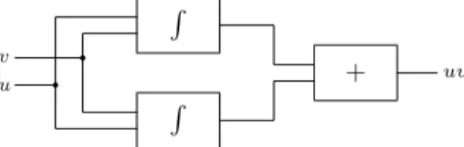
For the case of +, it is enough to use an adder and two input units connected to the adder to get the result. In the case of product, we use the circuit sketched in figure 5.1. R R + u v uv q q
Figure 5.1: A circuit that computes uv.
To show that this circuit works, one only has to consider the formula of integration by parts (for definite integration)
u(t)v(t) = Z t t0 u(x)dv(x) + Z t t0 v(x)du(x) + u(t0)v(t0).
Inductive step: consider now the two operators. Suppose that we have
f =CM(g, f1, ..., fk). Suppose, without loss of generality, that g has x1, ..., xs
and xs+d, ..., xk as LVs and AVs, respectively. Because the locked variables of
f are x1, ..., xm, we conclude that f1, ..., fscannot depend on xm+1, ..., xn. Let
xir
1, ..., xirα, and xjr1, ..., xjβr be the LVs and AVs of fr, for r = 1, ..., k, with ir
1< ... < irαand j1r< ... < jβr.
We have ir
α, jβr ≤ m, for r = 1, ..., s (and irα≤ m for r = s + d, ..., k). Using the
induction hypothesis, there exists, for r = 1, ..., k, a FF-GPAC Frthat generates
the function
fr(air
1, ..., airα, 0, ..., 0, ϕjr1(t), ..., ϕjrβ(t), 0, ..., 0),
(the actual order of the variables could be different, but this is not important for us). Now substitute in Fr, for s + d, ..., k, the input units associated to xt
by at, for t = 1, ..., m, respectively (hence, these FF-GPACs compute fr, with
the first m arguments fixed). We still denote these new FF-GPACs by Fr, for
r = 1, ..., k. Let
br= fr(air
1, ..., airα, 0, ..., 0, aj1r, ..., ajβr, 0, ..., 0),
for r = 1, ..., s. Also by the induction hypothesis, there exists a FF-GPAC G that computes the function
With these FF-GPACs, we can build a FF-GPAC that computes the com-position of functions. This is sketched in figure 5.2.
Fk Fs+d+1 Fs+d G .. . .. .
Figure 5.2: A circuit that computes the composition of functions.
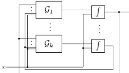
Finally, suppose that INT(F1, ..., Fk, G1, ..., Gk) is the description associated
to f. By similar arguments to the previous case, we can obtain FF-GPACs
G1, ..., Gmsuch that Gj computes the function
gj(a1, ..., am, 0, ..., 0, ϕn+1(t), ..., ϕn+k(t)).
Finally
˜
f (t) = f (a1, ..., am, 0, ..., 0, ϕn(t))
can be obtained by the FF-GPAC indicated in figure 5.3, where the integrator connected to Gi, for i = 1, ..., k, takes the following initial value
fi(a1, ..., am, 0, ..., 0).
To see that we can pick an appropriate enumeration of the integrators of the circuit represented in figure 5.3, pick appropriate enumerations for the various sub-FF-GPACs and then take the following general enumeration:
Z 1 , ..., Z k , G1, ..., Gk,
whereRi denotes the integrator connected to Gi, for i = 1, ..., k. Therefore, the
circuit indicated in figure 5.3 is a FF-GPAC.
Gk G1 .. . R R .. . x q q q q q q ·· ··
6
Conclusion
We have shown that Shannon’s GPAC and Pour-El’s alternative definition still present too many problems in order for them to be considered as appropriate mathematical models for analog computers. Therefore, we have introduced a new model (the FF-GPAC) that preserves the desirable properties of the GPAC (namely, it is a model based on circuits that preserves equivalence with differentially algebraic functions) but that has a “nice behavior”. We have further showed the relevance of this model by establishing full connections with a class of recursive functions over the reals.
Some questions can be considered. For example, can we introduce natural complexity measures in defining the FF-GPAC? Indeed, we saw in theorem 13 that the number of integrators in a FF-GPAC can be related to the order of the differentially algebraic function that it generates (a d.a. function of order
n can only be generated by a FF-GPAC with at least n integrators). This
result indicates that this task is apparently feasible, although possibly with some limitations.
The results proved in this paper can also be seen as a different route in order to establish connections with the classical theory of computation. In [3], [4], [5], several connections between recursive functions over the naturals and recursive functions over the reals are established. This work does not rely in the coding of Turing machines into some real numbers as in [8], [10], [15], and hence presents an alternative path to the traditional work in the field.
Acknowledgments. We would like to thank Cris Moore and Manuel Cam-pagnolo for several useful discussions related to this work. In particular, we acknowledge M. Campagnolo for the idea that would led to the concept of IR
-path.
This work was partially supported by FCT and FEDER via the Center for Logic and Computation - CLC, Laborat´orio de Modelos e Arquitecturas Computacionais - LabMAC, and is inserted in the FCT project ConTComp.
References
[1] V. Bush. The differential analyzer. A new machine for solving differential equations. J. Franklin Institute, 212:447-488, 1931.
[2] B. C. Carlson. Special Functions of Applied Mathematics, Academic Press, 1977.
[3] M. L. Campagnolo and C. Moore. Upper and lower bounds on continuous-time computation. In I. Antoniou, C. S. Calude, and M. J. Dinneen, editors,
Unconventional Models of Computation, UMC’2K, DMTCS, pp. 135-153,
Springer-Verlag, 2001.
[4] M. L. Campagnolo, C. Moore, and J. F. Costa. An analog characterization of the Grzegorczyk hierarchy. Journal of Complexity, to appear.
[5] M. L. Campagnolo, C. Moore, and J. F. Costa. Iteration, inequalities, and differentiability in analog computers. Journal of Complexity, 16(4):642-660, 2000.
[6] D. S. Gra¸ca. The General Purpose Analog Computer and Recursive
Func-tions Over the Reals, MSc thesis, IST/UTL, 2002. (available online at
http://w3.ualg.pt/~dgraca.)
[7] T. W. Hungerford. Algebra, Springer-Verlag, 8th printing, 1996.
[8] P. Koiran, M. Cosnard, and M. Garzon. Computability with low-dimensional dynamical systems. Theoretical Computer Science, 132:113-128, 1994.
[9] L. Lipshitz and L. A. Rubel. A differentially algebraic replacement theorem, and analog computation. Proceedings of the A.M.S., 99(2):367-372,1987. [10] C. Moore. Unpredictability and undecidability in dynamical systems.
Phys-ical Review Letters, 64:2354-2357, 1990.
[11] C. Moore. Recursion Theory on the reals and continuous-time computation.
Theoretical Computer Science, 162:23-44, 1996.
[12] P. Odifreddi. Classical Recursion Theory, Elsevier, 1989.
[13] M. B. Pour-El. Abstract computability and its relations to the general purpose analog computer. Transactions Amer. Math. Soc., 199:1-28, 1974. [14] C. Shannon. Mathematical theory of the differential analyzer. J. Math.
Phys. MIT, 20:337-354, 1941.
[15] H. T. Siegelmann. Neural Networks and Analog Computation: Beyond the
Turing Limit, Birkh¨auser, 1999.
[16] D. W. Stroock. A Concise Introduction to the Theory of Integration, Birkh¨auser, 3rd edition,1999.