Effects of Local Heat Input Conditions on the Thermophysical Properties of Super Duplex
Stainless Steels (SDSS)
José Adilson de Castroa*, Elizabeth Mendes Oliveirab, Darlene Souza da Silva Almeidaa,b, Glaúcio
Soares da Fonsecaa, Carlos Roberto Xavierc,d
Received: April 18, 2017; Revised: December 10, 2017; Accepted: December 10, 2017
The properties of the super duplex stainless steels (SDSS) are strongly affected by the thermal
history imposed by welding procedures. The controlled dual phase microstructure (ferrite and austenite) guarantee excellent mechanical properties such as mechanical strength and corrosion resistance,
in addition to small thermal expansion coefficient and high thermal conductivity. In this paper, we
newly proposed a model able to predict the thermal history of the welding pieces coupled with local
mechanical properties developed during welding procedure that combine the effects of temperature and phase changes during welding. We applied inverse method to fit the thermophysical parameters based on measured data. The model was verified by comparing measured and predicted temperature profiles using thermocouples located within the heat affected zone. Thus, an inverse method was implemented to obtain the parameters fitting for the grain growth evolution compatible with the final microstructure and grain size measured using SEM images and stereological techniques. We demonstrated that very small amount of non-equilibrium deleterious phases and nanosized precipitated are expected during
the welding procedures depending upon the local conditions of temperature, compositions and alloying dilution evolutions.
Keywords: Super duplex stainless steel (SDSS), heat input, thermal conductivity, heat capacity, mathematical modeling, non equilibrium, nanosized precipitate.
*e-mail: [email protected]
1. Introduction
Enhanced properties of the off shore materials are the main
subject to be addressed in order to attain safety and extend
service life of the equipments. Two aspects are of primary concern: corrosion and residual stress. Microstructure plays
a decisive role on both1,2. The accurate determination of the residual stresses during the steels welding and corrosion resistance during service are, therefore, subjects that need better attention due to their technological importance3-6. The super duplex stainless steels (SDSS) are enhanced materials that could be used in several applications that need higher performance3. Nevertheless, the welding process can introduce deleterious and non-homogeneous properties, which are critical and have limited some noble application3,7.
The SDSS are characterized by an excellent balance of the ferrite and austenite phases with size and distributions
that confers special properties for these materials. Yet, the
role of alloying elements can significantly modify their
properties on the local basis. The phases balance during the
welding procedure is a key feature for the final properties
developed in the joints of the pieces and equipments and
hence, their performance. The balanced ferrite and austenitic
phases on the SDSS can be strongly affected by the local
heat input and strict control of the thermal distributions is the technological and practical parameters that can be
handled in order to keep suitable temperature profile during
the welding procedure. Therefore, these combinations of balanced phases and elements dilution into the phases and
some rejection allowing the formation of fine precipitates can
confer excellent properties such as corrosion resistance and good toughness3,7,8. In welding process or working at elevated temperatures, secondary phases may appear as precipitates7,8. These compounds can be deleterious for steel properties at
heat affected zone, depending of the size and volume fractions
distributions. The principal precipitate that appears in this case is the sigma phase, although other precipitates such as chi
phase or nitrites could be encountered. It is well known that
the chi phase can be a precursor of the sigma phase which is also deleterious for the properties of SDSS7,8. The literature
on characterization of the chi and sigma phases are abundant
and indicated that these deleterious phases can be formed
aPrograma de Pós-Graduação de Engenharia Mecânica e Metalurgia, Universidade Federal
Fluminense, Av. dos Trabalhadores, 420, Vila Santa Cecília, CEP 27255-125, Volta Redonda, RJ, Brazil.
bDepartamento de Engenharia Metalúrgica, Centro Federal de Educação Tecnológica - CEFET-RJ,
23953-030, Angra dos Reis, RJ, Brazil.
cDepartamento de Engenharia Mecânica, Centro Universitário de volta Redonda, Av. Paulo E. A.
Abrantes, 1325, Três Poços, CEP 27240-560, Volta Redonda, RJ, Brazil
in large amount if the temperature is kept around 800ºC for times longer than 30 min7,8. This is not a typical time interval
on the critical zone for common welding process of small pieces. However, for large equipments and welding pieces
it is common to use multiple pass welding procedure and some regions can relay into the gap of temperature and time suitable to form the deleterious phases. Thus, the design of an
adequate welding procedure is important to make or repair the equipment to work under safety conditions9-12. In this work we propose an approach that could help on this task.
The heat input is a common measure and indication for the expected phases formed and distribution of the heat
affected zone (HAZ). Nevertheless, depending on the local
conditions of elements dilution and temperature distributions
non-equilibrium phases and nanosized precipitates can be
formed.
Models capable of predicting the local conditions and
possibility of deleterious phases being formed are welcome and can drive good practice for avoiding the non-uniformity of properties12-22. This paper is focused on this challenge. Thus, our work focused on the development of a computational tool for virtually simulates the welding procedure in order to give guidance for the onsite execution. The computational code is based on the simultaneous solution of the energy
equation coupled with the phase changes kinetics in order to predict the final phase balance. Additionally, an inverse
method is newly applied using measured values of materials properties and model adjustments are carried out for the super duplex stainless steel (SDSS).
Previous works have addressed the phase transformations and properties evaluation developed in the welding joints due to the heat input distributions9-23. Furthermore, the process simulation using numerical methods have been a fundamental tool for new developments. This approach
furnishes qualitative and quantitative analysis of the stresses
and prediction of the resultant microstructure and mechanical properties of the welds17-23. Thus, this study deals with the predictions of coupled phenomena of kinetic transformations under non-isothermal conditions for super duplex stainless
steel. The model consists of coupled differential equations and takes into account grain growth effects, permitting the
prediction of the progress of the phase balance and formation of deleterious phases simultaneously and correlates with local properties evolutions.
Thus, the present work is an attempt for numerically predicting the transformations coupled with local changes of properties occurring during the welding procedure of super duplex stainless steels. For this purpose, the kinetic model of Avrami-type with adjustable parameters is proposed7,8,13,16,24,25 and implemented using a computational code developed by
the author. The code is based on the finite volume method (FVM)26-28 implemented in Visual Fortran programming
language. It is important to mention that, to date, precise
properties such as thermal conductivity and heat capacity as functions of temperature and compositions are not available for the super duplex stainless steels. This confers to this study highly innovative features and technological importance.
Furthermore, the computer code used has been continuously
updated by the authors and applied for different materials
and welding conditions3,6,9-12. In this paper we introduce new features to improve the model capability such as routines for kinetics of phase transformations for super duplex stainless steels7,8.
2. Methods
The methodology adopted in this study considers the numerical implementation of the computational code
using specific routines for local phase transformations and thermophysical evaluations. In order to obtain suitable thermopysical properties for solving the energy equation
an inverse method is proposed with assumed boundary conditions. The selected measured transient temperatures are experimentally obtained in a controlled experiment and
used for solving the minimization problem, where the thermal
conductivities, k, and heat capacity, Cp, are unknowns. The
kinetics rate equations for the chi, sigma phases are used from
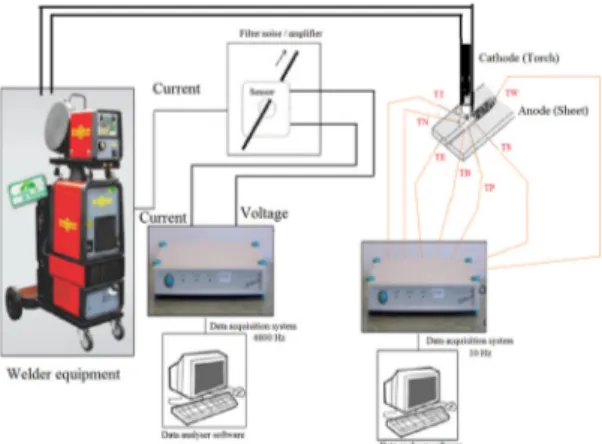
previously published work7,8.The experimental procedure is carried out with the automatic measurements and monitoring system schematically shown in Figure 1. The system is composed of a controlled welding module and multiple
acquisition data module for welding parameters of voltage, current and speed and a temperature acquisition module
where simultaneous transient measurements are recorded. Figure 2 shows the positions and arrangements of the inner temperature monitoring for the dynamic thermophysical
properties determination and model verification. A large number of transient temperature measurements at different
positions, designed for the inverse method proposed in the study, are used for both dynamic estimation of the
thermophysical properties and model verification.
Figure 1. Welding experimental arrangement and data acquisition
2.1 Numerical procedure
The temperature field is dynamically calculated during the
welding process evolution and the materials thermophysical
properties are continuously updated. The basic equations to model the process are presented by Equations (1)-(7). The
model takes into account the heat transfer by radiation, convection and conduction. The mass transfer due to consumable deposition and dilution within metal base
melting and solidification are considered and the properties
changes due to local composition and temperature are taken into account9-12. The temperature distribution is obtained by
solving the energy conservation, shown in Equation(1)9-12. In
Equation 1, ρ is the density, Cp is the specific heat capacity; k
is thermal conductivity, U→ is velocity field, which accounts
for buoyancy driven flows in the liquid pool or moving
mesh to attain the geometry changes due to the consumable deposition, T is the temperature field and S are all source or sink heat due to moving arc torch, phase transformations,
melting and solidification.
(1)
(2)
(3)
The model equations are completed with the formulation
of the heat source due to the torch and metal transfer mode. The heat input is supplied by the moving torch. We assume the well-known double-ellipsoid model9-13,22. The heat source is a combination of two ellipses in the front and rear
quadrants. Equations (4) and (5) present the volumetric heat flux distributions for the front and rear quadrants, respectively,
and their constant parameters. The coordinates are time dependent and gives spatial transient distributions22.
(4)
(5)
The total heat input Q = ηVI is determined by the operational parameters current (I), voltage (V) and thermal
efficiency η, respectively. The spatial distribution parameters
ff and fr are the fraction of the total heat received in the front
and rear quadrant, respectively. The parameters are chosen
attaining the relationship9-12,22, f
f + fr = 2. The heat input
constant parameters a,bf,c and br, are sellected to account for the torch heat distribution9-12. These constant parameters
sellected in this model are assumed fixed values, as shown
in Table 1. The factors ff and fr were assumed as 0.6 and 1.4 respectively while η was assumed 0.75 througout the all
cases analyzed3,9-12. The model parameters assumed in this study are presented for the cases considered in Table 1. The experimental design was sellected using the sinergic mode
where the voltage aimed fixed and the current slightly adjusted
for keeping constant welding power. The welding speed was changed by controlling the motion of the torch and thus, controlling the heat input. The constant parameters of the heat source model were kept constant, as shown in Table 1.
The initial condition is assumed with the whole workpiece at room temperature and the composition as received material.
The geometry of the bead is actualized for each time step after metal deposition and motion of the torch arc. The effects of convective and radiative fluxes are considered using Equations
6 and 7, respectively, by applying the boundary conditions.
(6)
(7)
In Equations (6) and (7), is the room temperature, ε(T) is
the emissivity and σ = (5.67x10⁻⁸ W .m-2 .K-4) is the
Stefan-Boltzmann constant. The effective heat transfer coefficient
accounting for the convective heat loss, h, was assumed 8 W .m-2 .k-1. In this study is assumed constant emissivity (0.45) during welding simulations3,9-23. The specific mass appeared
in Equation 1 is assumed constant as 7700 kg.m-3. The
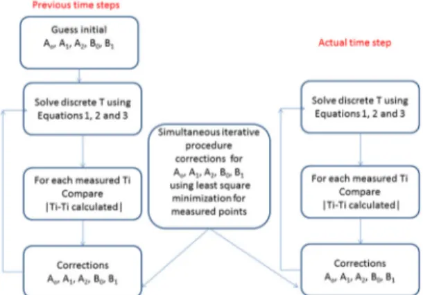
constants used in Equations 2 and 3 are obtained by iterative procedure using the optimization problem for corrections
of the constant parameters using transient measurements of the temperatures positioned within the working piece, as shown in Figure 2. The iterative process for determining the constants A0, A1, A2 and B0 and B1 is shown in Figure 3 for one time increment, involving backward and forward time
steps for solving the complete discrete equations based on
the measured values. This iteration process is carried out for the whole transient calculations and averaged values are
obtained and fitted for the equations 2 and 3 as temperature
dependent functions. Therefore, simultaneous measurements
of the temperatures for the same time step are required. The basic discrete equation used in this study is presented in Equations (8)-(12).
(8)
Figure 2. Temperature measurements arrangement using thermocouples
and numerical predictions for first welding pass (t=10s and heat
input 0.7 kJ mm-1)- central thermocouples dynamic measurements for estimating thermophysical properties.
( ( ))
t c Tp div cp U T" div k grad T S
2 2
t + t = +
Q
V
#S
X
& " %( )
C T
p=
A
0+
A T
1+
A T
2 2( )
k T
=
B
0+
B T
1( ), ( ), ( )
q x t y t z t
ab c f Q
e e e
6 3 r r r a x b y c z
3 3 3
r
2 2 2
r r
= - -
-R W S X T Y SX
( ), ( ), ( )
q x t y t z t
ab c f Q
e e e
6 3 f f f a x f y z
3 3b 3c
2 2 2
r r
= - -
-R W S X U Z SX
(
)
q
c=
h T
-
T
0(
)
q
r ( )TT
T
4 04
f
v
=
-( ) ( ) ( )T C T k T
T T T
y T T T
z T T T
2 2 2
pk P Pk P k
t T T S
Wk Pk Ek Sk kP Nk Bk Pk Tk
2 2
2
2
2 2 2
2
2 2 2
2
2 2 2
P k Pk k 2 3 2
T T T
t \ = - + + - + + - + T - -- - -- - - --
-T Y T Y T Y
# #
(9)
(10)
(11)
(12)
The values used in the right side of the Equations
(8)-(12) are measured and the left side after substitutions using
equations (2) and (3). The superscript k indicates the time step measured of the temperature values. The resulting system
of algebraic equations are solved for the unknown constants
and using the procedure schematically shown in Figure 3 for all transient measured values for the welding conditions shown in Table 1. The constants are then used on the direct method solution of the transient temperature distributions of the whole sheet and can be universally used for the SDSS.
2.2 Experimental procedure
We prepared samples of super duplex stainless steel (SDSS) sheets with dimensions of 60 x 210 x 8.0 mm to use in the experimental runs. The chemical composition of the main
elements was determined by the technique inductive coupled
plasma optical emission spectrometry (ICP-OES) for the as
received material, as shown in Table 2. The experimental procedure was carried out with thermocouples inserted within the specimen and the temperature recorded and used to apply the inverse method. The recorded data were used
to obtain the basic effective properties used to calculate the temperature field, thermal conductivity and heat capacity, k and Cp, respectively, applying Equations (2) and (3).
Three runs of experimental conditions were conducted for
different heat inputs, 0.7, 1.2 and 1.7 kJ.mm-1, respectively. The transient average temperature values were used and for each heat input the same position of the thermocouples
undergoes different thermal history, which was used to fit the constants of equations 2 and 3. Therefore a large number of
temperature values are measured and can be used for solving
the minimization problem obtained by applying the inverse
method with the unknown constants (A0, A1, A2, B0, B1) of
equations 2 and 3, respectively. The measured transient
temperatures obtained from the thermocouples 7 central
positions (TS, TN, TW, TE, TB, TT and TP) are used to generate 5 discretized equations for 5 sequential time steps,
which are solved for the unknowns A0, A1, A2, B0, B1, as
shown in Equations (8)-(12). This procedure is repeated
for a large number of time steps and the average values are computed. These computed values are now used for the direct
numerical method calculations of the temperature field. The
temperature history are compared for the whole transient calculation on the positions (T1,T2,T3,T4,T5 and T6) and
small adjustment are iteratively allowed for minimizing the average absolute difference of the measured and calculated
temperatures (see Figure 3).
The austenitic grain size plays important role on the
mechanical properties and during the phase decomposition
process. We applied a temperature-dependent rate equation, as shown in Equation (13), with the parameters obtained by measuring the final grain size of the HAZ previously
determined3.
(13)
( ) ( ) ( )
T C T k T
x T T T
y T T T
z T T T
2 2 2
Pk P Pk P k
t T T S
Wk Pk Ek S k P k N k B k P k Tk 1 1 1 2
1 1 1
2
1 1 1
2
1 1 1
P k P k k 1 2 1
T T T
t = - + + - + + - + T - -- -- - - --
-T Y T Y T Y
# # & & ( ) ( ) ( )
T C T k T
x T T T
y T T T
z T T T
2 2 2
P k
P Pk Pk
t TT
S
Wk Pk Ek Sk pk Nk Bk Pk Tk
2 2 2
P k
Pk k
1
T T T
t = - + + - + + - + T
-T Y T Y T Y
# # & & ( ) ( ) ( )
T C T k T
x T T T
y T T T
z T T T
2 2 2
P k P P k Pk t T TS
W k P k E k S k P k N k B k P k T k 1 1 1 2
1 1 1
2
1 1 1
2
1 1 1
Pk Pk
k
1 1
T T T
t = - + + - + + - + T + + + - -+ + + + + + + + + + +
T Y T Y T Y
# # & & ( ) ( ) ( )
T C T k T
x T T T
y T T T
z T T T
2 2 2
P k
P Pk p k
t T T S
Wk Pk Ek Sk kP Nk Bk Pk Tk
2 2
2
2
2 2 2
2
2 2 2
2
2 2 2
P k P k k 2 1 2
T T T
t = - + + - + + - + T + + + - -+ + + + + + + + + + + +
T Y T Y T Y
# #
& &
Table 1. Selected double ellipsoid model parameters and welding data
Voltage (V) Current (A) Speed (mm.s-1) Thickness (mm) Heat input (kJ.mm-1) Double-ellipsoid model constants (mm)
30 179 7.41 6.35 0.7 a = 5.35; bf= 2.3; c = 7.8; br= 14
30 178 4.33 6.35 1.2 a = 5.35; bf= 2.3; c = 7.8; br= 14
30 180 3.05 6.35 1.7 a = 5.35; bf= 2.3; c = 7.8; br= 14
25.7 170 6.76 8.00 0.5 a = 5.35; bf= 2.3; c = 7.8; br= 14
25.7 166 2.24 8.00 1.5 a = 5.35; bf= 2.3; c = 7.8; br= 14
25.7 169 1.59 8.00 2.2 a = 5.35; bf= 2.3; c = 7.8; br= 14
30 178 4.33 10.50 1.2 a = 5.35; bf= 2.3; c = 7.8; br= 14
30 179 4.33 6.35 1.2 a = 5.35; bf= 2.3; c = 7.8; br= 14
30 179 4.33 2.00 1.2 a = 5.35; bf= 2.3; c = 7.8; br= 14
Figure 3. Flowchart of the iterative procedure to estimate the constant
parameters for equations 2 and 3 based on discrete measurements
of transient temperatures
-The deleterious phase formation kinetic was modeled
as Avrami-type equation with the parameters previously
determined by Fonseca et al7. We applied the constants obtained using the published data for the mechanism 1, presented by Fonseca et al7, which is compatible with the welding typical times carried out on this study.
(14)
In Equation (14)Vv is volume fractions of the phases,
R is apparent activation energy, R is universal constant, t is residence time and T is temperature. The values obtained
from the data fitting for the mechanism 1, K0 = 1.54x10 20,
Q = 421 KJ .mol-1, and n = 2.68 were used for the computations
of the dynamic calculation of the transformed phases. In the
present model, the initial phase composition of the material,
chemical composition and average grain size are input
parameters for the model. Thus, when local transformations temperature is achieved the transformations are likely to occur following the local kinetic conditions.
3. Results and Discussion
3.1. Estimation of the thermophysical properties
for SDSS using inverse method
The welding predictions are strongly dependent on
the themophysical properties, as shown in equation (1).
This section discuss the results obtained for the constants
of the Equations (2) and (3) and the comparisons of
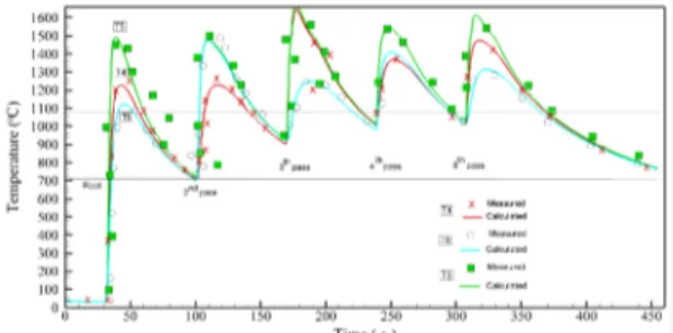
the model predictions for the recorded temperatures of the selected points where the thermocouples are positioned. Three different heat input were selected and the proposed method was applied. Figure 4, 5 and 6 show the comparison of the calculated and measured
transient temperatures for the heat input of 0.7, 1.2 and 1.7 kJ.mm-1, respectively, used to estimate the constants presented in Table 3. As can be shown in Figures 4, 5 and 6, the measured and calculated transient results are in close agreement for all compared results, which validates the proposed inverse method procedure used in this study. Therefore, the constants presented in Table
3 adequately represent the behavior of the SDSS during
the whole thermal cycle.
The evolution of the heat capacity and conductivity are presented in Figures 7 and 8, respectively, as functions of time and temperature for a measured position (TP). The calculated values of the thermal conductivity, k and capacity, Cp, were obtained after substitution of the
constants presented in Table 3 in the Equations (2) and
(3), respectively. As observed, the measured temperature
fitted well with the local predicted with the new constants
obtained in this study. The spatial variations of the thermal conductivity and heat capacity are presented in Figure 9
and 10, respectively, for the first pass showing the strong
dependence with the temperature variations. Similar results
are obtained for the analyzed cases, reflecting the effect
of temperature.
V
EXP
k t EXP
RT
Q
1
V
n 0
= -
T
-
T
-
Y
Y
Table 2. Super duplex stainless steel (SDSS) chemical composition used.
C (%) Mn (%) Si (%) P (%) S (%) Cr (%) Ni (%) Mo (%) Cu (%) N (%)
0.020 0.850 0.328 0.027 0.0009 24.890 6.820 3.720 0.156 0.278
PREN=%Cr+3.3×(%Mo)+16×(%N)=41.62 - Note: chemical analysis carried out using ICP-OES technique.
Figure 4. Transient temperature measurements and comparison with
numerical predictions after thermophysical properties determination using inverse method (heat input =0.7 kJ mm-1).
Figure 5. Transient temperature measurements and comparison with
numerical predictions using inverse method (heat input =1.2 kJ mm-1).
Figure 6. Transient temperature measurements and comparison with
3.2. Effects of welding parameters on deleterious
phases formation
The sigma phase formation in SDSS usually requires larger
times at during the cooling step at the range of 750-850 ºC. We applied model to the conditions and times where are expected
significant amount of this phase formation. Figure 11 shows the
comparison of sigma phase volume formation and those predicted
by the model under such conditions. As expected, the model fitted
well the experimental data in those conditions, therefore we can
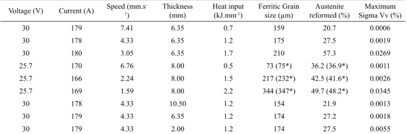
have confidence on the predictions under the welding procedures carried out in this study. The effects of welding parameters on the maximum volume fractions of phases on the HAZ are presented
in Table 4. The increase of the heat input promotes the increase
of the maximum grain size, austenite reformed and sigma
phases. The sigma and reformed austenite phases distributions for the intermediate heat input are shown in Figure 12 and 13, respectively. Table 4 shows the maximum values for all cases
analyzed and their respective welding parameters.
Table 3. Constants for the heat capacity (Cp) and thermal conductivity
(k) of super duplex stainless steel (SDSS) determined using the
proposed method (Equations 2 and 3).
A0 A1 A2 B0 B1
558.14 0.3253 0.000525 10.50 0.0108
Figure 7. Transient thermal conductivity predictions for position
TP using equation 2 and table 3 (heat input =1.2 kJ mm-1).
Figure 8. Transient heat capacity calculations at position TP using
equation 3 and table 3 (heat input =1.2 kJ mm-1).
Figure 9. Transient thermal conductivity (k) distributions during
the first welding pass (time = 32 s and heat input =1.2 kJ mm-1)
Figure 10. Transient heat capacity(Cp) distributions during the
finishing welding pass (time = 32 s and heat input =1.2 kJ mm-1).
Figure 11. Model predictions confronted with experimental
predictions of sigma phase under favorable formation conditions.
Figure 12. Grain size evolution resulted after the finishing welding
pass (heat input =1.2 kJ mm-1).
Figure 13. Predicted sigma phase evolution resulted after the
Table 4. Maximum sigma and reformed austenite phases volumes fractions and grain size predicted for the welding conditions
Voltage (V) Current (A) Speed (mm.s -1)
Thickness (mm)
Heat input (kJ.mm-1)
Ferritic Grain
size (µm) reformed (%)Austenite
Maximum
Sigma Vv (%)
30 179 7.41 6.35 0.7 159 20.7 0.0006
30 178 4.33 6.35 1.2 175 27.5 0.0019
30 180 3.05 6.35 1.7 210 57.3 0.0269
25.7 170 6.76 8.00 0.5 73 (75*) 36.2 (36.9*) 0.0011
25.7 166 2.24 8.00 1.5 217 (232*) 42.5 (41.6*) 0.0026
25.7 169 1.59 8.00 2.2 344 (347*) 49.7 (48.2*) 0.0345
30 178 4.33 10.50 1.2 154 21.9 0.0013
30 179 4.33 6.35 1.2 174 27.2 0.0018
30 179 4.33 2.00 1.2 174 27.5 0.0055
*Averaged measured values using 10 randomly samples (about 5% of dispersion for grain size and 2% for austenite volume fractions).
Figure 14. SEM image of the welding regions for heat input of
0.5 kJ mm-1.
Figure 15. SEM image of the welding zones for heat input of 1.2
kJ mm-1.
Figure 16. SEM image of the welding zones on the SDSS for heat
input of 2.2 kJ mm-1
Therefore the heat input and thickness are important
parameters to take into account during the adequate
selection of the welding procedure depending on the application29,30. The model presented in this study is an important tool to correctly design the suitable welding
procedure and control of the changes on the HAZ. The
simulation results indicated that, under the welding conditions considered, very small amount of sigma phase
is dispersed formed on the HAZ.
Therefore, the predicted amount is negligible, as can be seen in Figure 13 and Table 4. These results are in agreement with microscopic observation on the welded samples, which could not be observed for all cases
considered. Figure 14, 15 and 16 show SEM images of the welding regions used to estimate the grain size and phase
changes evolution. The results of the micrographs and the calculations present same trend. As can be observed, the
ferritic grain size increased as the heat input increased.
4. Conclusions
We proposed a coupled model for dynamically estimating the thermophysical properties during welding procedures of
the SDSS. The model was verified comparing experimental
measurements of the transient temperatures during welding
and the final microstructure. Local effects of heat input,
thickness and interpass temperatures were evaluated using the mathematical model. We found that very small amount
of deleterious phases could be formed on the HAZ during
welding of SDSS sheets (less than 15 of volume fraction). The amount of deleterious phases increased for interpass temperatures of 600ºC and smaller thickness for heat input of 1.2 kJ. mm-1.
5. Acknowledgements
The first author thanks to CNPq and FAPERJ for finantial support.
6. References
1. Zacharia T, Vitek JM, Goldak JA, DebyRoy TA, Rappaz M, Badeshia HKDH. Modeling of fundamental phenomena in
welds. Modelling and Simulation in Materials Science and Engineering. 1995;3(2):265-288.
2. Grong Ø, Shercliff HR. Microstructural modelling in metals
processing. Progress in Materials Science. 2002;47(2):163-282.
3. Almeida DSS, Queiroz AV, Xavier CR, Marcelo CJ, Castro JA, Oliveira EM. Modelo duplo-elipsoide acoplado a volumes finitos para simular a soldagem GMAW do aço inoxidável
SAF 2205. Tecnologia em Metalurgia Materiais e Mineração.
2016;13(2):148-156.
4. Souza GC, Silva AL, Tavares SSM, Pardal JM, Ferreira MLR, Cardote Filho I. Avaliação das propriedades mecânicas e da resistência à corrosão em soldas de reparo pelo processo GTAW
no aço inoxidável superduplex UNS S32760. Soldagem &
Inspeção. 2014;19(4):302-313.
5. Heinze C, Schwenk C, Rethmeier M. Numerical calculation
of residual stress development of multi-pass gas metal arc welding under high restraint conditions. Materials & Design.
2012;35:201-209.
6. Fonseca GS, Barbosa LOR, Ferreira EA, Xavier CR, Castro JA. Microstructural, Mechanical, and Electrochemical Analysis
of Duplex and Superduplex Stainless Steels Welded with the
Autogenous TIG Process Using Different Heat Input. Metals.
2017;7(12):538-559.
7. Fonseca GS, Oliveira PM, Diniz MG, Bubnoff D, Castro JA.
Sigma Phase in Superduplex Stainless Steel: Formation, Kinetics
and Microstructural Path. Materials Research.
2017;20(1):249-255.
8. Magnabosco R. Kinetics of sigma phase formation in a Duplex
Stainless Steel. Materials Research. 2009;12(3):321-327.
9. Xavier CR, Delgado HG Jr, Castro JA, Ferreira AF. Numerical Predictions for the Thermal History, Microstructure and Hardness Distributions at the HAZ During Welding of Low Alloy Steels.
Materials Research. 2016;19(3):520-533.
10. Demarque R, Castro JA, Xavier CR, Almeida DSS, Marcelo CJ, Santos EP, et al. Estudo Numérico e Experimental da Evolução Microestrutural e das Propriedades de Juntas Soldadas
de Vergalhões pelo Processo GMAW. Soldagem & Inspeção.
2015;20(4):434-445.
11. Demarque R, Castro JA, Xavier CR, Almeida DSS, Marcelo CJ, Santos EP, et al. Numerical and experimental study of the
microstructural evolution and the properties of joints welded
on rebars using the GMAW process. Welding International.
2017;31(6):425-434.
12. Castro JA, Xavier CR, Moreira LP, Sazaki Y. Modeling the Welding Process of the Low Alloy Ferritic Steels T/P23 and T/
P24. Advanced Materials Research. 2012;476-478(2):642-649.
13. Babu K, Prasanna Kumar TS. Comparison of Austenite
Decomposition Models During Finite Element Simulation of Water
Quenching and Air Cooling of AISI 4140 Steel. Metallurgical
and Materials Transactions B. 2014;45(4):1530-1544.
14. Gergely M, Somogyi S, Réti T, Konkoly T. Computerized
Properties Prediction and Technology Planning in Heat Treatment
of Steels. In: ASM Handbook. Volume 4. Materials Park: ASM
International. 1991; p. 638-656.
15. Paloposki T, Liedgust L. Steel emissivity at high temperatures.
VTT: VTT Information Service; 2005. 81 p.
16. Reti T, Fried Z, Felde I. Computer simulation of steel quenching
process using a multi-phase transformation model. Computational Materials Science. 2001;22(3-4):261-278.
17. Xavier CR, Delgado HG Jr., Castro JA. An Experimental and Numerical Approach for the Welding Effects on the
Duplex Stainless Steel Microstructure. Materials Research.
2015;18(3):489-502.
18. Xavier CR, Delgado HG Jr., Castro JA. Numerical evaluation of the weldability of the low alloy ferritic steels T/P23 and T/
P24. Materials Research. 2011;14(1):73-90.
19. Xavier CR, Campos MF, Castro JA. Numerical method
applied to duplex stainless steel. Ironmaking and Steelmaking. 2013;40(6):420-429.
20. Islam M, Buijk A, Rais-Rohani M, Motoyama K. Simulation-based numerical optimization of arc welding process for reduced
distortion in welded structures. Finite Elements in Analysis and Design. 2014;84:54-64.
21. Jalaal M, Ghasemi E, Ganji DD, Bararnia H, Soleimani S, Nejad MG, et al. Effect of temperature dependency of surface emissivity on heat transfer using the parametrerized perturbation
method. Thermal Science. 2011;15(Suppl 1):S123-S125.
22. Goldak J, Chakravarti A, Bibby M. A new finite element
model for welding heat sources. Metallurgical Transactions B. 1984;15(2):299-305.
23. Ashok Kumar K, Satish G, Lakshmi Narayana V, Srinivasa Rao
N. Development of mathematical model on gas tungsten arc welding process parameters. International Journal of Research
24. Avrami MJ. Kinetics of Phase Change. I: General Theory.
Journal of Chemical Physics. 1939;7(12):1103-1112.
25. Cahn JW. Transformation kinetics during continuous cooling.
Acta Metallurgica. 1956;4(6):572-575.
26. Karki KC, Patankar SV. Calculation procedure for viscous
incompressible flows in complex geometries. Numerical Heat
Transfer. 1988;14(3):295-307.
27. Patankar SV, Spalding DB. A calculation procedure for heat, mass
and momentum transfer in three-dimensional parabolic flows.
International Journal Heat Mass Transfer. 1972;15(10):1787-1806.
28. Melaaen MC. Calculation of fluid flows with staggered and
nonstaggered curvilinear nonorthogonal grids-the theory. Numerical Heat Transfer, Part B: Fundamentals. 1992;21(1):1-19.
29. Ferro P, Bonollo F. A Semiempirical Model for Sigma-Phase
Precipitation in Duplex and Superduplex Stainless Steels.
Metallurgical and Materials Transactions A. 2012;43(4):1109-1116.
30. Tavares SSM, Pardal JM, Lima LD, Bastos LN, Nascimento AM, Souza JA. Characterization of microstructure, chemical