Consumer credit analysis: a VAR/VECM methodology

2019

UNIVERSIDADE DE LISBOA

FACULDADE DE CIÊNCIAS

DEPARTAMENTO DE MATEMÁTICA

INSTITUTO SUPERIOR DE CIÊNCIAS

DO TRABALHO E DA EMPRESA

DEPARTAMENTO DE FINANÇAS

CONSUMER CREDIT ANALYSIS: A VAR/ VECM

METHODOLOGY

Inês Fernandes Claudina

Mestrado em Matemática Financeira

Dissertação orientada por:

2019

UNIVERSIDADE DE LISBOA

FACULDADE DE CIÊNCIAS

DEPARTAMENTO DE MATEMATICA

INSTITUTO SUPERIOR DE CIÊNCIAS

DO TRABALHO E DA EMPRESA

DEPARTAMENTO DE FINANÇAS

CONSUMER CREDIT ANALYSIS: A VAR/ VECM

METHODOLOGY

Inês Fernandes Claudina

Mestrado em Matemática Financeira

Dissertação orientada por:

i

ACKNOWLEDGMENTS

A sincere thank you to the following people.

I would like to start thanking to the faculty members of the master’s in financial mathematics for what they have taught me, and specially, to my thesis advisor Professor Diana Aldea Mendes. The door to Prof. Mendes office was always open whenever needed, she allowed this paper to be my own work but guided me in the right the direction whenever she thought I needed it.

I also want to thank to my colleagues Mariana, João and Francisco to help me through my Master, without all the study sessions, ideas exchange and companionship this experience would have been much harder and not so enjoyable. Then, I want to thank Nuno, that always encouraged me and kept me motivated through this process.

Finally, I must express my very profound gratitude to my parents for the continuous encouragement they have always given me, not only throughout my years of study and through the process of researching and writing this thesis, but at all times in my life, good or bad. This accomplishment would not have been possible without them. Thank you.

iii

ABSTRACT

The main objective of this dissertation is to present an empirical analysis that is able to describe the credit channel for households in Portugal, focusing on the disparities caused by the 2008 crisis. For this purpose, it was analysed a set of four times series including GDP (GDP), 3 months Euribor rate (EURIBOR), Inflation Rate (CPI) and Households Consumer Credit (CC) between the first quarter of 2003 to the last quarter to 2018. The data used was taken from Pordata website.

The subject in question begins with the study of the stationarity of the time series and the significance of the same followed by the implementation of the VEC model to answer several questions around this topic. It will be done an Impulse response function analysis for the most appropriate estimated model to assess the effect of an impulse (or shock) to the time series.

The main interest in the use of these models is the possibility of separate the endogenous and exogenous components of monetary policy to study the dynamic of time series in the long-term and measuring the response of variables to unexpected shocks.

v

RESUMO

O principal objectivo desta dissertação é apresentar uma análise empírica capaz de descrever o canal de crédito do sector privado em Portugal, com foco nas disparidades causadas pela crise de 2008. Para este propósito analisou-se um conjunto de quatro séries temporais, o Produto Interno Bruto (PIB), a taxa Euribor a 3 meses (Euribor), a taxa de inflação (IPC) e o crédito ao consumo do setor privado (CC) entre o primerio trimestre de 2003 e o último trimestre de 2018. Os dados utilizados foram obtidos no site Pordata.

Começa-se com o estudo da estacionaridade das séries temporais e a significancia das mesmas, seguido pela implementação do modelo VEC para responder a várias questões. Posteriormente será feita uma análise da função Impulso-resposta para o modelo estimado mais apropriado para avaliar o efeito de um impulso (ou choque) na série temporal.

O principal interesse no uso desses modelos é a possibilidade de separar os componentes endógenos e exogenas da política monetária para estudar a dinâmica das séries temporais a longo prazo e medir a resposta das variáveis a choques inesperados.

vii

CONTENTS

INTRODUCTION ... 1

1. THEORETICAL FRAMEWORK ... 2

1.1 CREDIT CHANNEL THEORY ... 4

1.2 THE PORTUGUESE ECONOMY ... 4

1.3 LITERATURE REVIEW ... 6

2. MACROECONOMETRICS: CONCEPTS AND MODELS ... 7

2.1 TIME SERIES ... 7

2.2 VAR MODEL………..………10

2.3 VEC MODEL ………...………..12

2.4 ADF, PP AND KPSS TESTS ... 13

2.5 COINTEGRATION AND GRANGER CAUSALITY ... 14

2.5.1. ENGLE-GRANGER TEST ... 15

2.5.2. JOHANSEN TEST ... 16

2.5.3. GRANGER CAUSALITY ... 17

2.5.4. IMPULSE RESPONSE FUNCTION ... 18

3. DATA AND RESULTS ... 19

3.1 EMPIRICAL ANALYSIS ... 20 CONCLUSION ... 33 REFERENCES ... 35 APPENDIX A ... 37 APPENDIX B ... 41 APPENDIX C ... 45 APPENDIX D ... 47

viii

LIST OF FIGURES

Figure 1 – The Circular Flow of Income ... 2

Figure 2 – Transmission mechanism of monetary policy ... 4

Figure 3 – Stationary time series (Juselius, 2006) ... 7

Figure 4 – Non-stationary time series (Juselius, 2006) ... 8

Figure 5 – Non-stationary behaviour ... 9

Figure 6 – VAR Model (Lutkepohl, 2005) ... ………..11

Figure 7 – Time Series logGDP, EURIBOR, CIP and logCC ... 20

Figure 8 – Time series consumer credit ... 21

Figure 9 – Histograms of the Series logGDP, EURIBOR, CIP and logCC ... 21

Figure 10 – Granger Causality Test ... 22

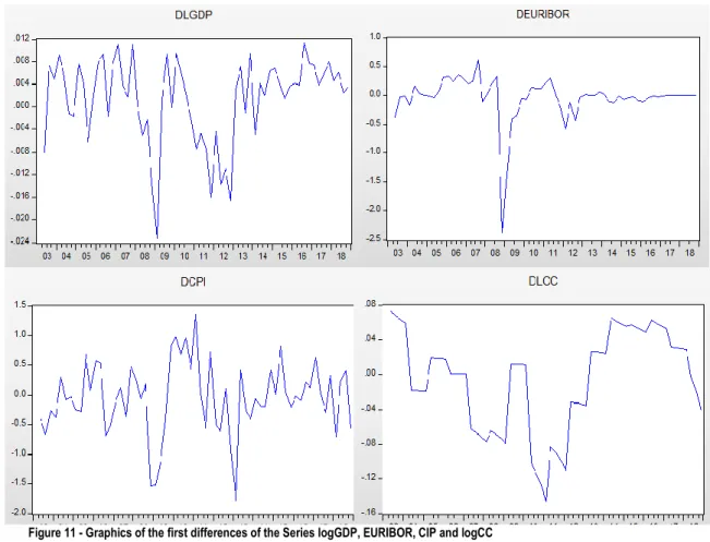
Figure 11 – Graphics of the first differences of the Series logGDP, EURIBOR, CIP and logCC ... 23

Figure 12 – Histograms of the first differences of the Series logGDP, EURIBOR, CIP and logCC ... 24

Figure 13 – VEC Residual Pormanteau Test for Autocorrelations ... 26

Figure 14 – VEC Residual Heteroskedasticity Test (Levels and Squares) ... 27

Figure 15 – VEC Residuals ... 28

Figure 16 – Cointegration relationship... 29

Figure 17 – Impulse Response Function EURIBOR ... 30

ix

LIST OF TABLES

Table 1 – Bank lending channel conditions ... 3

Table 2 – ADF, PP and KPSS Test Hypothesis ... 10

Table 3 – Linear correlation coefficients between variables... 22

Table 4 – Results for ADF, PP and KPSS Tests ... 23

Table 5 – Unit Root Test for the variables ... 24

Table 6 – Linear regression between variables ... 25

Table 7 – Johansen Trace Test ………..…25

Table 8 – Normalized cointegration coefficients ... 28

Table 9 – Unit Root Test ADF of the variable LGDP in level... 37

Table 10 – Unit Root Test PP of the variable LGDP in level ... 37

Table 11 – Stationarity Test KPSS of the variable LGDP in level ... 37

Table 12 – Unit Root Test ADF of the variable EURIBOR in level ... 38

Table 13 – Unit Root Test PP of the variable EURIBOR in level ... 38

Table 14 – Stationarity Test KPSS of the variable EURIBOR in level ... 38

Table 15 – Unit Root Test ADF of the variable CIP in level ... 39

Table 16 – Unit Root Test PP of the variable CIP in level ... 39

Table 17 – Stationarity Test KPSS of the variable CIP in level ... 39

Table 18 – Unit Root Test ADF of the variable LCC_TOTAL in level ... 40

Table 19 – Unit Root Test PP of the variable LCC_TOTAL in level ... 40

Table 20 – Stationarity Test KPSS of the variable LCC_TOTAL in level ... 40

Table 21 – Unit Root Test ADF of the variable LGDP - first difference ... 41

Table 22 – Unit Root Test PP of the variable LGDP - first difference ... 41

Table 23 – Stationarity Test KPSS of the variable LGDP - first difference ... 41

Table 24 – Unit Root Test ADF of the variable EURIBOR - first difference ... 42

Table 25 – Unit Root Test PP of the variable EURIBOR - first difference ... 42

Table 26 – Stationarity Test KPSS of the variable EURIBOR - first difference ... 42

Table 27 – Unit Root Test ADF of the variable CIP - first difference ... 43

Table 28 – Unit Root Test PP of the variable CIP - first difference ... 43

Table 29 – Stationarity Test KPSS of the variable CIP - first difference ... 43

x

Table 31 – Unit Root Test PP of the variable LCC_TOTAL - first difference ... 44

Table 32 – Stationarity Test KPSS of the variable LCC_TOTAL - first difference ... 44

Table 33 – R1: lcc_total c cpi ... 45

Table 34 – R2: lcc_total c euribor ... 45

Table 35 – R3: lcc_total c cpi ... 45

Table 36 – R4: cpi c euribor ... 46

Table 37 – R5: cpi c lgdp ... 46

Table 38 – R6: euribor c lgdp ... 46

Table 39 – Test Lags information criteria of Schwartz ... 47

xi

ABBREVIATIONS

CPI – Consumer Price Index

EBF – European Banking Federation ECB – European Central Bank

EFAP – Economic and Financial Assistance Programme EU – European Union

EURIBOR – Euro Interbank Offered Rate GDP – Gross Domestic Product

IMF – International Monetary Fund

HICP – Harmonized Index of Consumer Prices LHS – Left Hand Side

LR – Likelihood Ratio

MLE – Maximum Likelihood Estimation

OECD - Organisation for Economic Co-operation and Development OLS – Ordinary Least Squares

RHS – Right Hand Side VAR – Vector Autoregressive

1

INTRODUCTION

The constantly growing need for economic and financial information has been a major subject of study for investor groups, governments and even individuals participating in the financial markets that are looking for a basis for all their decisions. Forecasting economic indicators it is essential to the benefit of those directly or indirectly related to the local and international financial markets. Monetary policy can be a powerful instrument for the Central Banks and a subject of interest for economist and policymakers due its significant influence in

achieving price stability (low and stable inflation) and to help to manage economic fluctuations.

We live in a period of time characterized by change, both economic and social. The world changed more since the beginning of the XXI century than in the last seventy years. These permanents changes need an active response as a way of survival. Financial innovation emerges in a continuous process as a consequence of the transformations that the business world suffered.

As stated by Brinkmeyer (2014) the recent crisis of 2008 has presented a major challenge to banks, monetary policymakers and the stability of the financial system as whole all over the world. The latter phases are still ongoing and with different repercussions in different economies. The present master thesis, having in mind this point, will analyse the consumption credit behaviour in the case of Portugal, in the time period between 2003 and 2018

This dissertation is organized in 3 chapters. Chapter 1 is an introduction to the economic and financial concepts in the context of the recent crisis, and also makes a brief review to the literature relating the relationship between these concepts and the macroeconometrics models that will be used. Chapter 2 explores the concepts of time series, stationarity, cointegration and causality focused on the VAR/VECM model. The empirical data and the process implemented with the help of Eviews software in order to obtain the results are described in Chapter 3. The thesis is finalized with the presentation of the conclusions.

2

1. THEORETICAL FRAMEWORK

The global economic and financial crisis of 2008 that originated in the United States and the bankruptcy of the American investment bank Lehman Brothers in September of the same year had negative effects on several financial institutions worldwide, a process that became known as the subprime crisis. The subprime lending crisis had a domino effect in the economy and originated a global financial crisis, a banking crisis and sovereign debt crisis. The recent crises have changed the way that banks and monetary policymakers work, especially when it refers to the grant of credit.

One of the most important functions of a bank in an economy (and the most significant source of income for a bank) it’s theirs lending capacity and the crisis marked after the collapse of the bank Lehman Brothers putted it at risk and so the lending business had to be revaluated from the Banks and monetary policymaker’s perspective point of view with the ultimate goal to maintain price stability to reassure the effectiveness of monetary policy. The crises and all the economic, political and social issues that emerged from it raised several issues and questions on how banks will act in the future concerning lending restrictions and how to protect their volatility against Market anomalies/ discrepancies and captures the impact of the crisis on the role which bank characteristics play in the context of bank lending.

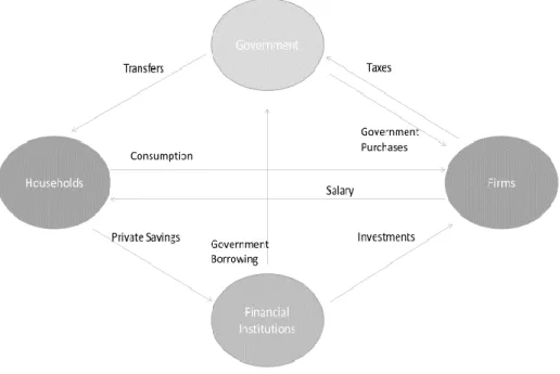
Figure 1 illustrates the circular flow of income, which represent a macroeconomic model that try to explain how money is distributed within an economy.

3 The Transmission channel of monetary policy is the process through which monetary policy decisions affect the economy and the price level. A State should be able to achieve macroeconomics objectives with the control of inflation, consumption, growth and liquidity as it is related to borrowing, consumption and spending by individuals and private.

There are several transmission channels of monetary policy decisions such as change in official interest rates, that affects banks and money-market interest rates, expectations, the asset prices, savings and investment decisions, the supply credit that leads to a change in aggregate demand and prices, that affects the supply of bank loans. The interest-rate channel it’s the one with the biggest impact as explains the effect of monetary policy on aggregate spending through changes in interest rates and assumes that the central bank can affect the short-term nominal interest rate given its monopoly power over the issuing of money and that investment and consumption expenditures are sensitive to changes in the real interest rate.

The bank lending channel suggests that banks play a special role in the transmission of monetary policy, this works by affecting banks’ assets (loans) and banks’ liabilities (deposits). The bank lending channel requires three conditions (Table 1) to be operational in the transmission of monetary policy (see, e.g., Bernanke and Blinder, 1988; and Kashyap and Stein 1994). The first one is that the central banks must be able to affect the supply of bank loans. Second, loans and bonds must not be perfect substitutes as a source for bank loans, describing firms’ dependence on bank-intermediated loans, there two conditions distinguish the bank lending view from the money view. The third condition states that prices must not be adjusted instantaneously after monetary policy changes – money is not neutral.

Condition 1 Condition 2 Condition 3

Central bank must be able to affect supply scheme of bank loans

Publicity issued debt and non-bank intermediated loans must not be perfect substitutes for bank loans

Prices must not adjust instantaneously (monetary policy must not be neutral)

Explanation

Banking sector must not be able to or willing to completely insulate lending portfolio from monetary policy shocks, either by:

- Switching from deposits to others forms of funding or - Selling securities

(liquid assets)

It must not be the case that firms are able to offset the decline in the supply of bank loans completely, i.e. without incurring additional cost, by borrowing more directly from household sector in public markets

Frictionless price adjustments would imply that policy rate changes immediately translate into price adjustments of an equal proportion and this must not be the case

4

1.1. C

C

T

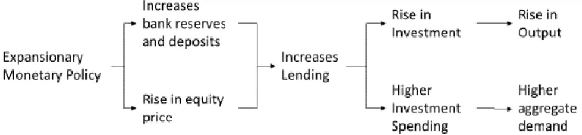
The transmission mechanism of monetary policy may be defined as the process by which asset prices and general economic conditions are affected because of monetary policy decisions. The modern financial system identified four channels of transmission of monetary policy: The Interest Rate Channel, the Asset Price Channel, the Exchange Rate Channel and the Credit Channel, which includes the Bank Lending Channel and the Balance Sheet Channel.

While the Bank Lending Channel focus on the importance of banks loans in the financial system, especially for certain borrowers that will not have access to the credit markets unless they borrow from banks (e.g. small firms and particulars), the Balance Sheet Channel operates through the balance-sheet positions of business firms, i.e. the loan borrower’s capacity to obtain loans. Figure 2 shows the transmission mechanism of monetary policy through the Credit Channel Theory. The Rise in output and higher aggregate demand are due to banks’ special role as lenders to classes of bank borrowers and the decrease in adverse selection and moral hazard problems, respectively.

1.2. T

P

E

The subprime crisis was the Biggest European crisis since the Great Depression (1929-1930) and became the crisis of sovereign debts, giving rise to the Greek and Irish bailout in May and November of 2010, respectively, and in April 2011 in Portugal held by Troika (the European Union (EU), the European Central Bank (ECB) and the International Monetary Fund (IMF)) leaving Portugal under the Economic and Financial Assistance Programme (EFAP) until May 2014.

At the time of the crisis the Portuguese economic situation was already problematic due to the excessive consumption growth, lower investment and savings from households, problems of international competitiveness, a growing public indebtedness and high current account deficits were reflected in a low economic growth. All that led Portugal quite vulnerable to the high volatility in the financial markets, the increase of the spread of the Portuguese sovereign debt was

5 so big that Portuguese banks no longer had access to foreign credit. The bailout reflected in several austerity measures applied, labour market reforms and reduced spending on education, health and pensions for Portugal.

The international financial crisis has demonstrated the seriousness of the imbalances accumulated over the previous decades and the barrier they represent for the growth of the Portuguese economy advent of the new millennium. The high unemployment and public debt, low wages, budget deficits, unsustainability of Social Security and constraints imposed to business and households by high debt level helped to create a snowball effect of the economic growth stagnation since the beginning of the XXI century.

This stagnation period from 2001 to 2014 can then be divided in two periods. From 2001 to 2007, before the national crisis that reflects the low economic growth and between 2008 to 2014, reflecting the impact of the international financial crisis and the euro area sovereign debt crisis and the resulting adjustment period, having as result the fall in the GDP.

6

1.3. L

R

The study of the transmission of the monetary policy is crucial for an economy and its interest was renewed after the 2008 crisis, inquiring the effectiveness and the determinants of the transmission channels.

The operating of monetary transmissons channels differs across different countries/ economic groups due to differences in the level of development of capital markets, the central bank autonomy and the country’s specific structural economic conditions. A quantitive approach can be a complement to historical event/data as it permits the measurement of the impact of monetary policy.

Jacobson et al. (2001) say that the two reasons behind the increase interest in empirical research of transmission mechanism of monetary policy was due to the deregulation of financial markets made monetary policy more oriented towards open markets operations than regulatory measures and that in many countries the emphasis in monetary policy has shifted towards explicit use of policy rules and monetary targeting.

The VAR model has received much attention as an instrument for modelling the monetary policy channels as it treats all linear relationships between variables as endogenous and the past values of these variables without imposing restrictions if they are dependent or independent, and, if necessary, it also allows exogenous variables on the model. furthermore, the VAR model allows to infer the effects from an impulse reponse function to one of the variables on all the other varaibles.

Several authors applied the VAR model in order to study the monetary policy channels: see for example, Canh (2016) and Lavally (2015), between others. ~

“Since the seminal work of Sims (1980), it has become a common practice to estimate the effects of the monetary policy on the real sector using vector autoregressions (VAR). This methodology avoids the problem of specifying the whole structural model of an economy and allows for the study of the dynamics of monetary policy shocks on the real economy. (…) The key aspect in applying the VAR methodology is the identification of the monetary policy shock.” (Aslandi, 2007).

This work aims to obtain impulse response functions that conform to the theoretical expectations, regarding the existence of the credit channel in the transmission of monetary distrubances, and are in line with the quantitative data previous obtained through the several tests.

7

2.

MACROECONOMETRICS: CONCEPTS AND MODELS

2.1.

T

S

A time series is a set of observations on the values of a variable timely ordered. A time series can refer to only one dependent or endogenous variable, if it refers to a univariate model, or to a set of observations if it is a multivariate model. The time series can be deterministic, when the output of the model is fully determined by the parameter values and the initial conditions or stochastic when randomness is present and variable states are not described by unique values, but rather by probability distributions. While linear regression requires a linear model and a linear equation has one basic form, a nonlinear equation can take many different forms. A relationship is spurious when two or more variables are associated but not causally related, this can be due to a third variable, known as the common response variable, or, it can just be a mere coincidence.

A time series it is called stationary if the mean, variance and covariance are all constant for each given time lag and do not show any trending behaviour (Figure 3), i.e., a stochastic process { 𝑋(𝑡) , 𝑡 ∈ 𝑇 } it is second order stationary if, ∀ 𝑡 ∈ 𝑇, we have:

1. 𝐸 (𝑋(𝑡)) = 𝜇

2. 𝑉𝑎𝑟(𝑋(𝑡)) = 𝜎2_{< +∞}

3. 𝐶𝑜𝑣(𝑋(𝑡1), 𝑋(𝑡2)) = 𝛾(𝑡1, 𝑡2) = 𝛾(|𝑡2− 𝑡1|) , 𝑡1, 𝑡2∈ 𝑇

A non-stationary time series refers to unpredictable data that cannot be modelled or forecasted as the results may have a spurious correlation. The data can be non-stationary if the

8 mean increases over time (the series should not be a function of time); the variance change with the time (heteroscedasticity) and the covariance is not constant as the spread becomes closer as the time increases. A typical non-stationary time series (with linear trend and non-constant variance) can be observed in figure 4.

The stationarity tests are very important and it’s essential that variables that are non-stationary be treated differently from those that are non-stationary as it can strongly influence its behaviour and properties and the use of non-stationary data can lead to spurious regressions. To have relevant results the non-stationary data needs to be transformed into stationary data, since the most of econometric/macroeconometric models are given for stationary data.

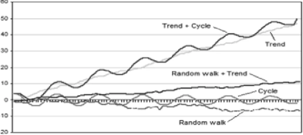
Non-stationary behaviours can contain trends, cycles, random walks or combinations of the three (see Figure 5). Random walk is the simplest example of a non-stationary time series. It is defined as the process where the current value of a variable is composed of the past value plus an error term defined by white noise (that is, a stochastic variable with null mean, variance one and zero autocorrelations) and it implies that the best prediction of the next period is the current value.

Figure 4 – Non-stationary series (Juselius, 2006)

9 The Random walk process it is also a well-known hypothesis about how financial prices move and can be formally stated as:

𝛾t= 𝛾t−1+ ɛt

where

𝛾

ɛ

ɛ

ɛt= Δ𝛾t= 𝛾t− 𝛾t−1

and is independent of past price changes. The accumulation of all past errors (below) can be written by successive backward substitution, highlighting that the price is indeed generated by the accumulation of purely random changes:

𝛾

∑ ɛ

𝑡

𝑖=1

The random walk is a difference stationary series since the first difference of

𝛾

We can deduce that the non-stationarity of a time-series generally can be induced by the trend (non-constant mean), and then we have a trend-stationary (or deterministic non-stationary) process or by the variance (and mean) and then we say that we have a stochastic non-stationary time series.

10 A deterministic non-stationary process can be transformed in a stationary one (or stabilized) by detrending the time series. In order to stabilize a stochastic non-stationary time series, we use the difference operator, that is

Δ𝛾t= 𝛾t− 𝛾t−1, Δ2𝛾t= 𝛾t− 𝛾t−2, …

If the time series is non-stationary in levels {

𝛾

the difference operator, then we say that the time series it is integrated of order d, I(d), where d is the order of integration.

The order of integration is also the number of unit roots contained in the series. For the random walk above, there is one-unit root, so it is an I(1) series. Similarly, a stationary series is I(0).

2.2.

VAR

M

Vector Autoregressive model (VARs) were popularised by Sims (1980) in Macroeconomics and Reality as an extension of the univariate autoregression model to the analysis of multivariate time series data describing the dynamic interrelationship among stationary variables. It is a multi-equation system where all the variables are treated as dependent (endogenous) and has three purposes: forecasting economic time series; designing and evaluating economic models; evaluating the consequences of alternative policy actions. Vector autoregressive processes are quite popular in econometrics and it became a standard framework due to its flexibility and simple models for multivariate time series data being advocated as an alternative to large-scale simultaneous equations structural models.

The bivariate VAR is the simplest example of this Model, where there are only two variables, y1t and y2t. Each of whose current values is dependent on different combinations of the

previous k values of both variables and error terms.

Y1t= β10+ β11y1t−1+ ⋯ + β1ky1t−k + α11𝑦2t−1+ ⋯ + α1k𝑦2t−k+ u1t ,

Y1t= β10+ β11y1t−1+ ⋯ + β1ky1t−k + α11𝑦2t−1+ ⋯ + α1k𝑦2t−k+ u1t ,

where uit is a white noise disturbance term with E(uit) = 0, (i=1,2), E(u1tu2t) = 0. The system can

be expanded to include g variables, y1t, y2t, y3t, …, ygt, each of which has an equation.

There are two important assumptions that must be considered from the time series data to set up a VAR model: stationary (that can be tested trough Unit Root Test) and the error normality and independence.

11 Steps to perform a VAR:

1. Test stationarity of data and degree of integration 2. Determination of lag length

3. Test the Granger causality 4. Estimation of VAR 5. Variance decomposition 6. Forecasting

Advantages of VAR modelling:

• Easy to estimate and good forecasting capabilities;

• There’s no need to indicate which variables are endogenous or exogenous - it considers that all variables are endogenous. This is a very important point due to the constraints to identify certain variables as exogenous;

• Easy to test for Granger non-causality;

• It allows the value of a variable to depend on more than just its own lags or combinations of white noise terms, making VARs more flexible than the standard univariate AR models – implying that they may be able to capture more features of the data;

• Pre-determined variables include all exogenous variables and lagged values of the endogenous variables – it is possible to simply use OLS separately on each equation confirmed that there are no contemporaneous terms on the RHS of the equations; Problems of VAR modelling:

• VARs are a-theoretical, since they use little economic theory information about the relationships between the variables to guide the specification of the model. Thus, VARs cannot used to obtain economic policy prescriptions;

• Not clear the appropriate lag length for the VAR to be determined;

12 • A lot of parameters. If there are K equations, one for each K variables and p lags of each of the variables in each equation, (K + pK2_{) parameters will have to be estimated. For}

relatively small sample sizes, degrees of freedom will rapidly be used up, implying large standard errors and therefore wide confidence intervals for model coefficients.

• It is essential that all the components in the VAR are stationary, however many advocates of the VAR approach recommend that differencing to induce stationarity should not be done as will toss information on any long-run relationships between the series away. There are two methods that are used to choose the optimal lag length: cross-equation restrictions that uses block F-test and information criteria that uses the likelihood ratio (LR).

2.3.

VEC

M

In the case that the time series are not stationary the VECM (Vector Error Correction Model) should be used instead as allows consistent estimation of the relations among the series and can consider any cointegrating relations among the variables as it has the coefficient of the error correction term incorporated into the model.

Given a VAR(p) of I(1): xt= ϕ1xt−1+ ⋯ + ϕpxt−p+ ϵt ,

The Error correction representation form is: 𝛥xt= ∑𝑝−1𝑖=1 ϕiΔxt−i+ ϵt,

where ϕj= − ∑𝑝𝑖=𝑗+1 ϕi, j=1, …, p -1

and 𝛱 = −(I − ϕ1+ ⋯ + ϕp) = −𝜙(1)

Steps performs an VECM

1. Determination of lag length 2. Test the Granger causality 3. Cointegration degree test 4. Estimation of VECM 5. Variance decomposition

The error correction term becomes more difficult to interpret, as it is not obvious which variable it affects following a shock.

13

2.4.

ADF,

PP

KPSS

T

The stationarity will be tested trough the unit root tests, like Augmented Dickey-Fuller (ADF) and Phillips-Perron (PP), and stationarity test, Kwiatkowski–Phillips–Schmidt–Shin (KPSS). The ADF Test is one of the best known and frequently used unit root tests and it is based on the model of the fist-order autoregressive process (Box, Jenkings, 1970), that is:

𝛾t= φ1𝛾t−1+ ɛt, t= 1, …, T

where φ1 is the autoregression parameter, ɛt is the non-systematic component of the model that

fits the characteristics of the white noise process. The null hypothesis of the ADF and PP test is: H0: φ1= 1

Which is expressed as an I(1), meaning that the process is non-stationary as it contains a unit root. The alternative process is

H1: | φ1 | < 1,

and it’s expressed as I(0), i.e., the process does not contain a unit root and it is stationary. The PP Test it’s an improvement from ADF Test as it incorporates an automatic correction to allow for autocorrelated residuals, considering breaks structures and volatility. The two tests provide similar conclusions.

The KPSS Test shows if a series is stationary around a mean or linear trend or is non-stationary due to a unit root. The null hypothesis is

H0: φ1= 0

for the test is that the data is stationary and the alternate hypothesis for the test H1: | φ1 | < 0

is that the data is not stationary. This test is a linear regression:

𝑥

= r

+ β

𝑡 + ɛ

,

breaking up the series into three parts: a deterministic trend (t), a random walk (rt) and a stationary

14 The use of stationarity and unit root tests are known as confirmatory data analysis. The null and alternative hypotheses under each testing approach are as follow (Brooks(2012)):

ADF/ PP KPSS

H0: yt ~ I(1) H0: yt ~ I(0)

H1: yt ~ I(0) H1: yt ~ I(1)

Table 2 - ADF, PP and KPSS Test Hypothesis

There are four possible outcomes: a) Reject H0 and Don’t Reject H0

b) Don’t Reject H0 and Reject H0

c) Reject H0 and Reject H0

d) Don’t Reject H0 and Don’t Reject H0

To have a relevant conclusion we should have outcome a) or b), which would be the case when both tests concluded that the series is stationary or non-stationary, respectively. Otherwise it would mean that there’s a confit in the results.

2.5.

C

G

C

We say that we are in the presence of cointegration if there is at least one stable, long-term, non-spurious relationship between a set of non-stationary time series. Cointegration considers the long-term properties (behaviour) of the model, not explicitly dealing with short-term dynamics. For this purpose, error correction models (ECM and VECM) have become very popular in the last decades. The dynamics part of the VECM describes the short-run effects and the cointegration relation describes the long-term relation between the non-stationary time series in the model.

The behaviour of cointegrated processes can be easily explained in the following way: treated individually, each process contains a unit root and has shocks with permanent impact. However, when combined with another series, a cointegrated pair will show a tendency to revert towards one another. Cointegration and error correction provide the tools to analyse temporary deviations from long-run equilibria.

Engle and Granger (1987) says that the components of a (k x 1) vector, Yt, are

cointegrated of order (d,c), Y ~ CI(d,c) if all Y elements are integrated of order d, I(d) and if exists at least one non-trivial linear combination, z, of this variables, that’s like I(d - c), where d ≥ c > 0, that is:

15

β′Y

= Z

~ I(d − c),

where β is the cointegration vector and it’s usually considered the case with d = b = 1. The cointegration level r it’s the same as the number of linearly independent cointegration vectors. The cointegration vectors are the columns of the cointegration matrix β′ such as:

β′Y

= Z

,

if all variables are I(1) and 0 ≤ r < k. For r = 0 the elements of vector Y are

non-cointegrated.

In this dissertation it will be considered the Engle-Granger and the Johansen cointegration methodologies, since they have been the most commonly used for cointegration analyses. The Ordinary Least Squares (OLS) estimation is used for the Engle-Granger method, while the VECM is estimated by the Maximum Likelihood Estimation (MLE) procedure.

The variables might be not cointegrated in the log-run, but still be related in the short-run – in order to understand short-run interdependence among the variables it will be performed the Granger causality tests. Each one of this topic will be briefly presented in what follows.

2.5.1. E

-G

T

The Engle-Granger test is a single-equation method used to determine whether there is a cointegrating relationship between two variables (Engle and Granger, 1987). Supposing that ût

are the residuals of the estimated model, the hypotheses for the Engle-Granger test for cointegration are:

• H0: ût ̴ I(1) – Non-stationary residual and no cointegration between variables.

• H1: ût ̴ I(0) – Stationary residual and cointegration between variables

Steps to perform Engle-Granger Test:

1. Determine the order of integration of the two variables (based on Unit root tests). 2. If the variables are both integrated of order one, I(1), cointegration is theoretically

possible. If the variables have a different order of integration, it can be concluded that cointegration is not possible.

3. Estimate the long-run, static relationship (equilibrium) by running the OLS linear regression, given by the general equation: Yt= βxt+ ut, where Yt and xt are the times

16 4. Test the residuals of the regression for unit root. The variables are cointegrated when the

null hypothesis (above) is rejected.

5. If the variables are cointegrated, estimate an error-correction model.

The major’s critics to this method are that it can only identify one cointegration vector at a time and the choice of the dependent variable may guide to different conclusions.

2.5.2. J

T

This test is an improvement to the Engle-Granger test. The Johansen method relies on a vector autoregression (VAR) model. A VAR is a system regression model which includes more than one dependent variable. Every variable is regressed on a combination of its own lagged values and lagged values of other variables from the system. Here, the simplest form is presented, where k denotes the number of lags included (Brooks, 2008):

Y

= β

y

+ β

y

+ ⋯ + β

y

+ u

,

where Yt is a vector of variables and yt−k is the lag of order k of the variable Yt. The VAR model

will be differentiated to be transformed into a VECM, that is:

Δy

= Πy

+ Γ

+ Δy

+ Γ

Δy

+ … + Γ

Δy

+ u

,

where  =∑ βj 𝑘

𝑗=1 − I𝑔 and Γ𝑖 = ∑ βj 𝑖

𝑗=1 − I𝑔.  is denoted the long-run coefficient matrix

and is of type (g×g). We can decompose the matrix  as the product  where (g×r) contains the cointegrating vectors while (g×r) gives the “loadings” of each cointegrating vector in each equation. We denote by r the rank of matrix . Now

(a) If r = g, then all-time series in Yt are stationary (no cointegration)

(b) If r = 0, then there is no long run relationship between the elements of Yt (no cointegration)

(c) If 0 < r < g, then there are multiple cointegrating vectors

The Johansen cointegration test is based on the rank of the matrix  evaluated via its eigenvalues (rank = number of nonzero eigenvalues). The eigenvalues of the long-run coefficients matrix are denoted by i and are written in descending order, that is:

17 If the variables Yt are not cointegrated, then, the rank of matrix  will not be significantly different

from zero, so i = 0  i.

The test statistics for cointegration are formulated as 𝜆𝑡𝑟𝑎𝑐𝑒(𝑟) = −T ∑ 𝑙𝑛(1 − 𝜆̂ )𝑖

𝑔 𝑖=𝑟+1

𝜆𝑚𝑎𝑥(𝑟, 𝑟 + 1) = −T 𝑙𝑛(1 − 𝜆̂𝑟+1)

where 𝜆̂𝑖 is the estimated value for the ith ordered eigenvalue from the  matrix. trace tests the

null that the number of cointegrating vectors is less than equal to r against an unspecified alternative. trace = 0 when all the i = 0, so it is a joint test.

max tests the null that the number of cointegrating vectors is r against an alternative of r+1.

The hypotheses for the Johansen method are:

• H0: no cointegration against the alternative of cointegration.

• H1: cointegration against the alternative of cointegration.

It’s very important to choose the optimal lag length, as the critical values of the method are quite sensitive to the same, and whether a constant term and time trend should be included, or not.

2.5.3. G

C

“Granger causality is a statistical method for studying casual links between [2] random variables” (Granger, 1969), determining whether one time series is useful in forecasting another. The term causality means that there is a correlation between the current value of one variable and that’s variable previous values. This test is based on a standard F-test and determinates if changes in one variable cause changes in another variable. If the previous values of X can predict the current value of Y, it’s said that variable X “Granger cause” variable Y.

Using a VAR model as an example, that is:

Y

= β

y

+ β

y

+ ⋯ + β

y

+

x

+

x

+

x

+ u

,

For this equation if all α – coefficients on lagged values of X are significant it means that “X Granger causes Y”. It’s called unidirectional causality if X Granger causes Y and Y doesn’t cause X, and bidirectional causality if X causes Y and vice versa (Brooks, 2008). The test statistic

18 follows a 𝑋2 _{distribution, with p (the optimal number of lags) degrees of freedom under the null}

hypothesis.

The hypotheses for the Granger causality test are: • H0: α1 = α2 = … = αp = 0 (“X does not Granger cause Y”)

• H1: at least one of α – coefficients ≠ 0 (“X does Granger cause Y”)

Granger Causality test can only show if two variables have significant impact on each other, it doesn’t give any information on how long it will last. An impulse response analysis can give an answer to this.

2.5.4. I

R

F

Impulse response analysis is widely used in econometric analyses, which uses vector autoregressive models. The Impulse Response Function (IRF) method is used to describe the evolution of a model’s variables in reaction to a shock in one or more variables. The impulse responses (IR) are used to ger a better understanding of the model’s dynamic behaviour. The IRF for a linear VAR model is made through its moving average representation that is also the forecast error impulse response function, that can be mathematically obtained by:

ϕi = ∑𝑖𝑗=1 ϕi−1Aj i=1, 2, ...

with ϕ0 = IK and Aj = 0 for j > p, where p is the lag order of the VAR model and K is the number

19

3. Data and Results

The present work consists of the econometric analysis of four time series that characterize the monetary policy in Portugal. The data it is comprised between the first quarter of 2003 and the last quarter of 2018, consists in 64 observations and was downloaded from the Portugal Central Bank site. We are going to apply VAR and VEC models in order to get the reaction of the variables to external shocks, by analysing the associated impulse response function. We are applying the EViews software in all the performed analysis. As it is usual in the Economic field the difference in the price series will be worked in logarithms instead of levels. It will be considered a level of significance of 5%.

Variables:

• Gross Domestic Product (GDP) for Constant Prices (in Millions) is the monetary value of all the goods and services produced within the geographic boundaries of a country during a specific period, normally one year. The GDP growth rate is an important indicator of the economic performance of a country (Time Serie: LogGDP).

• EURIBOR or the Euro Interbank Offer Rate is based on the interest rates at which a panel of European banks borrow short-term funds from one another, and it’s communally used as benchmarked reference for bank loans. This Market interest rate is calculated daily by the European Banking Federation (EBF) and published by Reuters. The oscillation of the EURIBOR interest rates evolves accordingly the reference rate practiced by the ECB but this can be also influenced be others external factors, such as, the demand and supply variation, the economic growth and the inflation rate. It will be considered the 3 months EURIBOR rate (Time Serie: EURIBOR).

• Inflation Rate: “Inflation measured by consumer price index (CPI) is defined as the change in the prices of a basket of goods and services that are typically purchased by specific groups of households. Inflation is measured in terms of the annual growth rate and in index” OECD (Time Serie: CPI).

• Households Consumer credit or consumer debt (in Millions) is a debt that a person incurs when purchasing a service or good, being the credit card the most common form of consumer credit. We will analyse the loan supply and loan demand data as certain events impact on factors that influence both at the same and to better understand the supply-side or demand-side factors (Time Serie Log CC_total).

20

3.1

E

A

The first step in our analysis consist in the graphical representation of the 4 economic variables in consideration. From Figure 7 we observe that none of the variables are characterized by a global linear trend, instead of this, several increasing and decreasing patterns are present. The variance it is quite smooth, which is typical to quarterly data.

1.6 2.0 2.4 2.8 3.2 3.6 2004 2006 2008 2010 2012 2014 2016 2018 LCC_TOTAL -1 0 1 2 3 4 5 6 2004 2006 2008 2010 2012 2014 2016 2018 EURIBOR 10.62 10.64 10.66 10.68 10.70 10.72 10.74 10.76 2004 2006 2008 2010 2012 2014 2016 2018 LGDP -2 -1 0 1 2 3 4 2004 2006 2008 2010 2012 2014 2016 2018 CPI

Figure 7 - Time Series logGDP, EURIBOR, CIP and logCC

The variable GDP doesn’t show a clear linear trend, since there’s a structural break in the last quarter of 2012 followed by a significant growing tendency period until the last quarter of 2018. The EURIBOR time series has an upright break from 2007 to 2008 followed by a decreasing trend which seems to stabilize in the last two years. The CPI time series also shows a break structure in the middle of 2009 and after that some more turbulent behaviour. The graphic of LCC variable it is given by a smooth curve, decreasing during the crises period and showing a recovery tendency beginning with 2014.

21

Figure 8 – Time series consumer credit

As it can be seen from Figure 8, the mortgage loans had a bigger variation and impact in the overall consumer credit during the studied period than the consumer credit and other purposes variables.

The next step it is the analysis of the descriptive statistics of the considered variables.

We observe that GDP, CPI and CC are normally distributed since we do not reject the null hypothesis of Jarque-Bera. All variables have a platykurtic distribution and small negative skewness, except Euribor, that is moderate positive asymmetric.

22 As per Jarque-Bera test the variable EURIBOR doesn’t follow a normal distribution for a level of significance of 5%, however the distribution is normal for a level of significance of 1% as H0 is not rejected. As so, it will be considered that all variables are Normally distributed.

We have below the table of linear correlation coefficients between the considered variables. We can observe positive correlation between all variables, with the highest correlation between Euribor and Households Consumer credit (0.6673), followed by Euribor and CPI (0.5881).

LCC_TOTAL EURIBOR LGDP CPI

LCC_TOTAL 1.000000 0.667392 0.456590 0.383195 EURIBOR 0.667392 1.000000 0.293009 0.588140 LGDP 0.456590 0.293009 1.000000 0.149092 CPI 0.383195 0.588140 0.149092 1.000000

Table 3 – Linear correlation coefficients between variables

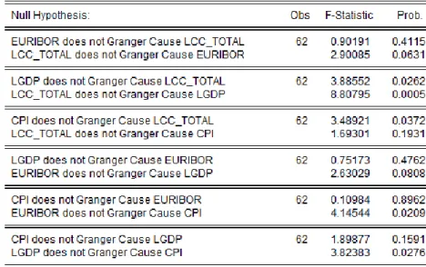
Figure 10 shows the Granger causality relation between the time series. It seems to exist several causality relationships between the variables, namely: Lcc_total Granger causes Euribor (for a confidence level of 10%), Lcc_total Granger causes lgdp, Cpi Granger causes Lcc_total, Euribor Granger causes lgdp (for a confidence level of 10%), Euribor Granger causes cpi and Lgdp Granger causes cpi. We observe that GDP and Consumer Credit are the only two variables characterized by a bidirectional Granger causality. We also observe that highly correlated variables are also Granger causal, in this case.

23 We conclude that exists a short time relationship between the variables, given by the causality effect between each other. In practice, when we establish Granger causality (or not), policy prescriptions might be suggested in order to encourage (or not) the provision of credit.

It will now be tested the stationarity of the series through the Unit Root Tests ADF and PP and the stationary test KPSS. The variables are considered in levels, with Intercept and maximum lags number equal to 4. The results for the three Tests can be find below, in Table 4:

ADF PP KPSS

LGDP 0.4989 0.6383 0.117859*

EURIBOR 0.5756 0.6338 0.723321

CPI 0.0771 0.0964 0.471588

LCC_TOTAL 0.2350 0.6988 0.623313

Table 4 – Results for ADF, PP and KPSS Tests *H0 is Rejected with a confidence level α = 5%

For ADF and PP Tests as p-value is bigger than 0.05, H0 is not rejected and as so the

series have a unit root and in consequence are non-stationary. For KPSS Test, for a confidence level of 5% all series are non-stationary, and the null hypothesis is rejected, since the test statistics it is lower than the critical values.

Since all the time series are non-stationary we have to apply the first difference operator and study the returns for the four series.

24 From Figure 11 we can observe that the mean is constant, but the variance increases. A negative “outlier” it is observed for the first difference of EURIBOR in midd 2008. Steepest decreasing values are present also for the growth rate of GDP and CPI in mid of 2008.

Figure 12 shows the histograms and the basic statistics of the first difference of the considered variables. CPI and LCC are normally distributed with zero mean, based on the Jarque-Bera test. The GDP is negatively asymmetric and leptokurtic. Finally, the EURIBOR it is also skewed to the right and with a very high kurtosis coefficient. An outlier can be observed.

ADF PP KPSS

LGDP 0.0000 0.0000 0.166573

EURIBOR 0.0000 0.0000 0.070910

CPI 0.0000 0.0000 0.049785

LCC_TOTAL 0.0301 0.0244 0.225301

Table 5 – Unit Root Test for the variables

For the Unit Root Tests ADF and PP, the P-value is smaller than 0.05, H0 is rejected and

so the series don’t have unit roots and they are all stationary. For KPSS Test, for a confidence level of 5% all series are stationary, and the null hypothesis is not rejected. We conclude than, that all variables are integrated of order 1, I(1).

25 In what follows we will study if the time series are cointegrated, or not, using the two methodologies defined by Engle-Granger and by Johansen.

We recall that Engle-Granger methods requires to analyse if the linear combination between two non-stationary variables (that is, the linear regression) produce a stationary time series (that is, the residuals). The output of all the simple linear regression models between the pairs of variables and the unit root test for the associated residuals are presented in Appendix C. Table 6 is the sum of these regressions, showing the p-value of the ADF unit root test applied to the residuals. lcc_total c cpi 0.4980 lcc_total c euribor 0.2625 lcc_total c lgdp 0.4019 cpi c euribor 0.0072 cpi c lgdp 0.0870 euribor c lgdp 0.7753

Table 6 – Linear regression between variables

It seems that there is a cointegration relationship between the variables cpi and Euribor as the p-value is smaller than 5% for the residuals unit root test. For the remaining variables, since the p-value is bigger than the test critical values (for all confidence levels) the null hypothesis of unit root is not rejected and so the residuals are non-stationary meaning that there is no additional cointegration relationship between the studied variables.

This statement will be confirmed (or not) by running in EViews the Johansen Trace Test, which is shown in Table 7:

Hypothesized

No. of CE(s) Eigenvalue

Trace Statistic

0.05

Critical Value Prob.**

None* 0.450527 60.09028 47.85613 0.0024

At most 1 0.235960 24.76135 29.79707 0.1701 At most 2 0.139211 8.882386 15.49471 0.3764 At most 3 0.000643 0.037962 3.841466 0.8455 Trace test indicates 1 cointegration eqn(s) at the 0.05 level

* denotes rejection of the hypothesis at the 0.05 leve ** MacKinnon-Haug-Michelis (199) p-values

Table 7 – Johansen Trace Test

At the 5% significance value, the trace test concluded in favour of one cointegration relation among the four variables, that is, there exist only one relationship which drive the long-run behaviour of the system.

26 Now, since there is one cointegration relationship between the variables, we are going to use a VECM instead of a VAR analyses. The VECM will identify long-run and short-run dynamics of the banking lending. First, we will test for the optimal lag number, which is two in our case, based on the information criteria of Schwartz (see Appendix D). Next the model VECM(4,2) will be estimated by the Maximum Likelihood method and the residuals are checked for independence (Figure 13), homoscedasticity (Figure 14) and normality.

From the VECM output (Appendix D), we can observe the short-run behaviour, that is, about 1% of disequilibrium it is corrected each quarter by changes in the consumer credit. In the same way, 9%, 0.5% and 34% of disequilibrium will be corrected each quarter by changes in the Euribor, GDP and CPI variables, respectively. The coefficients of the error correction term of Consumer Credit, Euribor and GDP variables are almost all insignificant, but the coefficient of CPI are significant. These means that if a disturbance occurs in the system, then, the change of CPI variable will have significant conservative force tending to bring the model back into the equilibrium state when it is going around.

VEC Residual Portmanteau Tests for Autocorrelations Null Hypothesis: No residual autocorrelations up to lag h Date: 09/01/19 Time: 20:13

Sample: 2003Q1 2018Q4 Included observations: 61

Lags Q-Stat Prob.* Adj Q-Stat Prob.* df 1 0.768944 --- 0.781760 --- --- 2 11.09346 --- 11.45626 --- --- 3 27.44556 0.4941 28.65416 0.4302 28 4 45.84515 0.3955 48.34494 0.3018 44 *Test is valid only for lags larger than the VAR lag order.

df is degrees of freedom for (approximate) chi-square distribution after adjustment for VEC estimation (Bruggemann, et al. 2005)

Figure 13 – VEC Residual Pormanteau Test for Autocorrelations

From Figure 13 we can see that the residuals are independent up to lag 2, based on the Portmanteau test. We check this by observing the p-values, which are higher than 0.05, and so, we do not reject the null of no residual autocorrelation

Figure 14 illustrates another residual test, namely the heteroscedasticity test. The null hypothesis is: residual variance is constant (or homoscedastic), which it is not rejected, since the p-value is higher than 0.05.

27 VEC Residual Heteroskedasticity Tests (Levels and Squares)

Date: 09/01/19 Time: 20:15 Sample: 2003Q1 2018Q4 Included observations: 61 Joint test: Chi-sq df Prob. 207.9042 180 0.0756 Individual components:

Dependent R-squared F(18,42) Prob. Chi-sq(18) Prob. res1*res1 0.275721 0.888260 0.5944 16.81896 0.5356 res2*res2 0.200555 0.585356 0.8901 12.23383 0.8349 res3*res3 0.412854 1.640690 0.0933 25.18407 0.1199 res4*res4 0.177050 0.501995 0.9423 10.80005 0.9026 res2*res1 0.501877 2.350919 0.0114 30.61450 0.0319 res3*res1 0.396522 1.533142 0.1264 24.18783 0.1490 res3*res2 0.174265 0.492431 0.9471 10.63014 0.9094 res4*res1 0.348736 1.249442 0.2692 21.27288 0.2659 res4*res2 0.201738 0.589682 0.8869 12.30599 0.8310 res4*res3 0.215158 0.639664 0.8467 13.12464 0.7841

Figure 14 – VEC Residual Heteroskedasticity Test (Levels and Squares)

The normality assumption cannot be attained because of the outlier present in the Euribor time series. Figure 15 illustrates the residuals of all variables. We can include a dummy variable in order to vanish the outlier, but this way we will improve artificially the model, and, however, the statistical outlier it is not a numerical error, it is a true economical phenomenon.

28 -.12 -.08 -.04 .00 .04 .08 2004 2006 2008 2010 2012 2014 2016 2018 LCC_TOTAL Residuals -2.5 -2.0 -1.5 -1.0 -0.5 0.0 0.5 2004 2006 2008 2010 2012 2014 2016 2018 EURIBOR Residuals -.015 -.010 -.005 .000 .005 .010 2004 2006 2008 2010 2012 2014 2016 2018 LGDP Residuals -2.0 -1.5 -1.0 -0.5 0.0 0.5 1.0 1.5 2004 2006 2008 2010 2012 2014 2016 2018 CPI Residuals VEC Residuals

Figure 15 – VEC Residuals

The cointegration relation between CPI and Euribor it is shown in Table 8. The cointegrating vector represents the positive relationship existing in the long-run between the 3-months nominal interest rate and consumer price inflation and the negative relationship with GDP.

This cointegration vector is a Fisher-type equation (that is, defines the one-for-one adjustment of the nominal interest rate to the expected inflation rate). In the euro area institutional framework this vector can be interpreted as a monetary policy reaction function, i.e., a Taylor rule describing the behaviour of the European Central Bank that sets the interest rate with the only objective of stabilizing the rate of consumer price inflation around a given target.

Normalized cointegrating coefficients (standard error in parentheses)

LCC_TOTAL EURIBOR LGDP CPI

1.000000 -0.090580 4.343800 -0.527891 (0.06871) (3.83756) (0.09302)

29 -2.0 -1.5 -1.0 -0.5 0.0 0.5 1.0 1.5 2.0 03 04 05 06 07 08 09 10 11 12 13 14 15 16 17 18 Cointegrating relation 1

Figure 16 – Cointegration relation

Once we validated the VECM(4,2) we can proceed to the impulse response function analysis to test the effect of perturbations on the variables.

First, we will give one standard deviation shock to the Euribor time series (Figure 17). The responses of GDP time series to the one standard deviation shock on Euribor is reflected by a short-term 0.3% quick increase, followed by a decreasing tendency and finally the turn back to the equilibrium after around three years. The CPI inclines in response to tightened Interest Rate conditions. The effect of Euribor restrictions on CPI reaches a peak after around one year and fades away after around three years.

The response of the Consumer Credit time series to the one standard deviation shock on Euribor it is more volatile. The first reaction observed it is the increase of the consumption credit, with more-less a quarter duration, which can be viewed as the normal reaction to novelty. After a short period of time, the consumer credit will decrease, about 2%, that is, a cautionary reaction of the consumer, and after, will slowly recover, taking around 10 quarters to get back to the stationary level. This confirms the existence of the relationship between interest rates and consumption. Usually, Central banks try to keep the interest rate below some threshold value and this way believes in the increase of the household consumption.

30 -.10 -.05 .00 .05 .10 2 4 6 8 10 12 14

Response of LCC_TOTAL to EURIBOR

-.010 -.005 .000 .005 .010 2 4 6 8 10 12 14 Response of LGDP to EURIBOR -.4 -.2 .0 .2 .4 2 4 6 8 10 12 14

Response of CPI to EURIBOR

Response to Nonfactorized One S.D. Innovations ± 2 S.E.

Figure 17 – Impulse Response Function EURIBOR

It will also be applied one standard deviation shock to the Consumption Credit time series. Figure 18 shows that the three-time series behave similarly, with moderate shock variation and they all take around 2 years to get back to equilibrium. The CPI and the Euribor variables initially

31 decrease some percentage points as consequence to the shock in the Consumer Credit, that is, a statistically significant reaction can be observed in the model. The one standard deviation shock to Consumption Credit causes the most significant decrease in the CPI time series (around 10%) for a period of 4 quarters after which the effect dissipates and an increasing tendency will be dominant in the next quarters. The maximum impact of the innovation in CC is experienced at quarter 3 and 2 for CPI and Euribor variables, respectively.

These are important pieces of information about the relationships between the time series in the VAR/VECM model. The GDP reaction it is to increase, attaining the maximum value, that is, about 1% at quarter 12, after which it will decrease. This reflects that the impact of consumer credit on output growth is clearly positive in short run. Recall also the bidirectional Granger causality and the high correlation coefficient between these two economic variables, reflecting the contemporary and short-run relation between them.

This way, from the analysis of the impulse response function, we can account for the relation between the credit and the business cycle given by the macroeconomic variables and to conclude that the credit it is important in explaining output fluctuations.

32 .000 .004 .008 .012 .016 .020 .024 2 4 6 8 10 12 14 Response of LGDP to LCC_TOTAL -.2 .0 .2 .4 2 4 6 8 10 12 14

Response of CPI to LCC_TOTAL

.0 .2 .4 .6

2 4 6 8 10 12 14

Response of EURIBOR to LCC_TOTAL

Response to Nonfactorized One S.D. Innovations ± 2 S.E.

33

CONCLUSION

This study focused on the credit channel theory in order to determine the effectiveness of transmissions mechanisms of monetary policy in Portugal during the last 16 years. To achieve this, the following variables were studied: Euro Interbank Offer Rate (EURIBOR), Consumer Price Index (CPI), Gross Domestic Price (GDP) and Households Consumer Credit, or consumer credit.

Looking to the graphic representation of the variables, the effects of the crisis is quite notable, even though, noticing in different periods/ ways for different variables. The consumer credit to households started to decrease in 2007, having an abrupt contraction until the end of 2008. This was due to the monetary policy barrier imposed, not for a declining in the demand. Ten years after and the consumer credit in Portugal is still below of the values before the crisis. The Euribor rate started to decrease after the crisis (more significantly in 2009) reaching, a never seen before, negative values in 2015, this was an unconventional monetary policy used to mitigate the financial crisis effects. The impact of the crisis in the GDP was first seen in 2008, however the lowest value of the same was in 2012, when the impact of the crisis already made itself felt in the Portuguese Economy and this reflects the status of the Portuguese Economy in the period followed by the crisis. The Index Price to Consumer had a tremendous decrease in the middle of 2009, followed by a turbulent period since 2013.

All the series are non-stationary while testing the stationarity of the same in levels (contains a unit root), however all variables are integrated of order 1, I(1). A Vector Error Correction (VEC) model was used as there was one cointegration relationship between the variables Euribor and CPI.

All the variables are correlated and there were several causality relationships between the variables. It was studied the Granger causality and the conclusion was that GDP and Consumer Credit are the only two variables characterized by a bidirectional Granger causality and they are also the variables that have the higher correlation coefficient. There is a short time relationship between all the variables, given the causality effect between each other. The Johansen test confirmed that there is only one cointegration relation between variables.

From the Impulse response function, it was intended to verify how the endogenous variables respond to exogenous shocks effects applied to the Euribor and consumer credit variables. This way, we can account for the relation between the credit and the business cycle given by the macroeconomic variables and to conclude that the credit it is important in explaining output fluctuations.

34 In conclusion, it is important to mention that there are some points that can be explored in the continuation of this dissertation that would add more value to the same, as the analysis of the same methodology but for other countries within the Eurozone. This would enable to crosscheck the results with the Portuguese reality and analyse the impact of the variables in different countries. Moreover the separation of the consumer credit in demand and supply can also give more insight to the monetary policy and bank lending channels in the Portuguese economy.

References

35

REFERENCES

Aslandi, O., (2007), The optimal monetary policy and the channels of monetary transmission mechanism in CIS-7 countries: the case of Georgia, Charles University

Brinkmeyer, H., (2014), Drivers of Bank Lending; New Evidence from the crisis, Springer Gabler

Brockwell Peter J. and Davis, Richard (2002), Introduction to time series analysis and forecasting, Springer, N. York

Brooks, C., (2008), Introductory Econometrics for Finance, 2nd ed., Cambridge University Press.

Canh, N., (2016), Monetary Policy Transmission and banks lending channel in Vietnam. PHD Thesis’s, University of Economics Ho Chi Minh City

Dickey, D. A., Fuller, W. A., (1979), Distribution of the estimators for autoregressive time series with a unit root, Journal of the American Statistical Association 74, 427-431

Engle, R. F., Granger, C. W. J., (1987), Co-integration and error correction: Representation, estimation and testing, Econometrica 55, 251-276.

Granger, C., (1969), Investigating causal relations by econometric models and cross-spectral methods, Econometrica, Vol. 37, No. 3, 424–438

Jacobson T, Jansson, P., Vredin A., and Warne A. (2001), A VAR Model for Monetary Policy Analysis in a small open Economy, Journal of Applied Econometrics, pages 487-520.

Johansen, S. (1992), Cointegration in Partial Systems and the Efficiency of Single Equation Analysis, Journal of Econometrics,

Juselius, K., (2007), The Cointegrated VAR model: Methodology and Applications, Oxford Univ Press.

Lavally, M., (2015), Investigating the effectiveness of transmission mechanisms of monetary policy in Sierra Leone. Master’s Thesis, The University of Namibia

Lutkepohl, H., (2005). New Introduction to Multiple Time Series Analysis (2nd edn.).Springer-Verlag: Berlin.