Estud. Econ. vol.38 número1

(1)

 ViViane Luporini

Resumo

Esse artigo analisa o canal juros do mecanismo de transmissão monetária sobre o produto, preços e taxa de câmbio na economia brasileira dos anos 90 através dos efeitos de uma redução inesperada na taxa básica de juros em um sistema de vetores auto-regressivos. Os principais resultados obtidos são: a) um choque monetário afeta imediatamente a atividade econômica, reduzindo a taxa de crescimento do PIB; b) a inflação e a taxa de câmbio são afetadas somente após um intervalo de tempo, e a inflação assume uma tendência declinante somente dois meses após o choque de juros; c) os resultados são robustos quando controlados para condições internacionais, preço das commodities ou outras medidas de inflação e atividade econômica; d) choques monetários afetam significativamente a volatilidade do produto e da inflação no modelo padrão; e) choques monetários afetam significativamente a volatilidade da relação dívida/PIB no modelo de controle.

PalavRas-chave

política monetária, mecanismo de transmissão monetária, Brasil

abstRact

This article presents evidence on the interest channel of the monetary policy for the Brazilian economy of the 1990s analyzing the effects of an unexpected change in the baseline interest rate on output, prices and the exchange rate in a vector autoregression system. Our main results are: a) a tightening in the monetary policy affects economic activity immediately, reducing the rate of growth of real GDP; b) the exchange rate and prices are affected only after a time interval, with inflation assuming a downward trend only two months after the monetary shock; c) results do not change when the specification is controlled for international conditions, commodity prices or other measures of inflation and economic activity; d) monetary shocks have a significant impact on the volatility of output and inflation in the benchmark model e) monetary shocks have a significant impact on the volatility of the debt/GDP ratio in the control-model.

KeywoRds

monetary policy, monetary transmission mechanism, Brazil

Jel classification E52

 _{professora do instituto de economia da universidade Federal do rio de Janeiro (uFrJ) e pesquisadora do Cnpq.}

en-dereço para contato: instituto de economia - ie, uFrJ – praia Vermelha – avenida pasteur, 250, sala 103, urca – rio de Janeiro – rJ. Cep: 22290-240. e-mail: viviane.luporini@ie.ufrj.br.

(2)

1. IntRoductIon

This paper presents evidence on the interest channel of the monetary policy for the Brazilian economy of the 1990s. Most economists tend to agree that actions by the monetary authority have real effects on the economy, altering the time path of real ou-tput and employment at least in the short run. On the empirical level, several studies have indeed shown that contractionary monetary policy actions, usually characterized by increases in the baseline nominal interest rate, tend to be followed by reductions in economic activity while expansionary actions are usually accompanied by increments in production and employment [see for example, Friedman and Schwartz (1963); Romer and Romer (1989); Cook and Hahn (1989); Sims (1992); Cochrane (1998); Barth and Ramey (2000)]. The reasons for this “empirical regularity” have been the subject of substantial controversy and produced a large literature on why and how changes in monetary policy may affect real variables (Blanchard,1990). Although the dispute may in fact reflect different views on how the real world actually works, the main explanations for the non-neutrality of monetary policy have been centered on informational issues, problems of signal extraction and expectation formation on one side, contracts, rigidities (nominal and real) and coordination problems on another. Theoretical disagreements standing, the important question from the policymaker’s point of view is not so much why monetary policy is not neutral, but how the main aggregates in the economy respond to actual changes in the monetary instruments available.

(3)

This paper follows the international empirical literature in terms of the methodology and examines the response patterns of main economic variables to an unanticipated tightening in the Brazilian monetary policy through a vector autoregression system of equations (VAR). Our analysis differs from Minella’s in three important ways. First, our benchmark specification includes the exchange rate as one of the endoge-nous variables in the model. Since the early 1990s, as the Brazilian economy began to open to international trade, this variable has become an important component of internal prices as well as monetary policy decision-making. Second, given the well-known sensitivity of impulse response functions to different specifications, the paper presents a sequence of alternative specification schemes providing a robustness analysis for the results. Finally, the paper sheds some light on how unexpected mo-netary policy shocks have contributed to the volatility of the economic aggregates in the model. The benchmark model finds that a tightening in the rate of change of the nominal selic rate has an immediate effect on economic activity, reducing the rate of growth of real GDP and a delayed effect on the rate of inflation, the main declared goal of the policymaker.

The paper is organized as follows. The second section presents the theoretical model of the VAR system, the third presents the evidence on the interest channel of the monetary policy, the fourth section brings the robustness analysis for the results ob-tained by the benchmark model and discusses the so-called “price-puzzle”. The fifth section describes the effects of the monetary shock on the volatility of the economic aggregates of the model and the sixth section concludes the article.

2. thE ModEl

A monetary shock is identified as the disturbance term in the general equation:

( )

t t t

S

=

f I

+σε

(1)

where s represents the monetary authority’s policy instrument, the baseline interest rate or some monetary aggregate, I represents the information set available to the po-licymaker at time t ,

σε

is a random variable representing a monetary shock and f is a function, assumed linear, relating the policy instrument s to the information It.

(4)

with unfulfilled expectations formed by private economic agents [Ball (1995), Chari, Christiano and Eichenbaum (1998)], exogenous variations in the monetary policy due to technical factors such as corrections in the preliminary data used by the Central Bank when making policy decisions (Bernanke and Mihov, 1995).

A widely used strategy for estimating the effects of monetary policy shock is to adopt the recursiveness assumption that the monetary shocks are orthogonal to the infor-mation set I used by the policymaker and then estimate the dynamic responses of the variable of interest to a monetary policy shock. This assumption is convenient because it justifies estimating the dynamic responses as a two-step procedure: first, the mo-netary policy shocks are obtained by the fitted residuals of the ordinary least squares regression of s on variables in the information set I; then, the dynamic response is estimated by regressing the variable of interest against current and lagged values of the policy shocks estimated in the first step. This two-step procedure is, moreover, summarized by an asymptotically equivalent system of vector autoregressions (VAR) [Christiano et al. (1999)].

Consider a VAR for the vector of variables

Z

_t:

t q t q t

t

B

Z

B

Z

u

Z

=

₁ ₋₁

+

....

+

₋

+

, and

Eu u

_t _t'

=

V

(2)

where

u

_t is uncorrelated with variables observed in period t-1 and earlier.

Ordinarily least squares of each equation in (2) produce consistent estimates of the coefficients and the v can be estimated from the fitted residuals.

Assume that the vector of disturbances in the VAR is related to the economic shocks

t

ε

according to

A u

0 t

= ε

t, where

A

0 is an invertible square matrix. '

t t

E

ε ε =

D

,

with d a positive definite matrix. Then, premultiplying (2) by

A

0, gives:

....

t t q t q t

A Z

0

=

A Z

1 ₋1

+ +

A Z

₋

+ ε

(3)

where

A

i, i= 0, 1, … , q is a matrix of constants;

B

i

A

i

1 0

−

=

, i=1,….,q, and

( )

₁ `

0 1 0

− −

=

A

D

A

V

.

The responses of

Z

t+hto a unit shock in the elements of

ε

tis given by:

h h

A

−

γ = γ

1

(5)

where

γ

his the solution to the difference equation

γ = γ + γ + + γ

h

B

1 h−1

B

2 h−2

...

B

q h q− ,

h = 1,2, … , with initial conditions

γ =

0

I

, the identity matrix,

γ

−1

=

γ

−2

=

...

=

γ

−q

=

0

.

The recursive assumption that the monetary shocks are orthogonal to the information set I used by the policymaker restricts

A

₀.

Although the recursiveness assumption is not sufficient to identify all the elements of

0

A

, it is sufficient to identify the dynamic response of

Z

_t to a monetary shock. By

selecting a lower triangular matrix with nonnegative terms on the diagonal such that

( )

A

V

A

− −1 '

=

0 1

0 , the dynamic responses of the variables in

Z

t will be invariant to the ordering of variables prior to the last variable in the information set (or the last varia-ble ordered in the VAR). It is worth noting that in the absence of further restric-tions, the dynamic responses to shocks to the other variables in the system simply re-flect the normalization of

A

0 adopted.

3. REsPonsEs to PolIcy shocks: thE EvIdEncE

There are basically two branches in the applied literature on the monetary trans-mission mechanism. The first one usually identifies the monetary policy shocks as innovations to some monetary aggregate, the monetary base, the money stock or M2 [Barro (1977), Reichenstein (1987), Cochrane (1994)]. The second trend, inter-prets policy shocks as innovations to the baseline interest rate [Bernanke and Gertler (1995), Bernanke and Blinder (1992), Christiano, Eichenbaum and Evans (1994, 1999)]. As most of the applied literature analyses the American case, the authors employ the federal funds rate as an indicator for the monetary policy. Peersman and Smets (2001) use the three-month interest rate as the monetary policy instrument for an analysis of the Euro area.

The Brazilian monetary authorities have been using the open-market interest rate as its main policy instrument. For this reason, the policy instrument considered in the analysis is the short-run interest rate (selic).

(6)

Real/US dollar exchange rate; the overnight market interest rate (Selic). These varia-bles are denoted by output, inflation, erate and interest, and were log-transformed to facilitate interpretation. Exception is made to the interest rate, which is measured in percentage points. The inflation rate was negative for September of 1995 (-1.08 per-cent). In order to apply the log operator, a constant c= 1.1 was added to the inflation rate over the whole period. This procedure is usual and does not affect the coefficients of interest as the added constant simply alters the intercept of the inflation regression equation. Data for the robustness analysis include an index for world exports, the U.S. Prime rate, a consumer price index (IPCA), an index for industrial production; the internal debt/GDP ratio, a commodity price index and the price for crude oil. The details for the series used are presented in the appendix.

3.1 unit Root tests

Before estimating the vector autoregression system, the variables must be tested for the order of integration. As suggested by Hayashi (2000), the unit root tests were perfor-med on a constant only, unless there is strong evidence of a deterministic time trend. This was the case for the output variable. The results are presented in Table 1.

The Augmented Dickey-Fuller (ADF) and Phillips-Perron (PP) tests have indicated that Inflation, Erate, commodity, oil, debt, us Prime, World Exports, and the IPca Index have unit roots at the 5% significance level; output, Interest and the Production Index do not have unit roots and may be considered stationary processes. Both the ADF and PP tests are known to have poor finite-sample properties (Hayashi, 2000, p. 601). The Dickey-Fuller-Generalized Least Squares test (DF-GLS), which has better finite-sample properties and good power, confirm the unit root results for Inflation, Erate, commodity, oil, debt, us Prime, World Exports and IPca Index, and indicate the presence of a unit root for Interest at 5% and output at 1%. The Production Index

remains stationary in level. In accordance to the unit root tests results, all variables in the system will be treated as integrated of first order, I(1).1

(7)

taBlE 1 – unIt Root tEsts: adF, PP and dF-Gls

Unit Root Tests Augmented Dickey-Fuller and Phillips-Perron

Variables Sample Det. Terms Test Stat Critical Values

ADF PP 1% 5% 10%

Output 1990:03-2001:08 c, trend -4.457 -4.996 -4.026 -3.443 -3.146

Inlation 1990:03-2001:08 -2.352 -2.788 -3.479 -2.883 -2.578

Erate 1990:03-2001:08 -1.209 -1.081 -3.479 -2.883 -2.578

Interest 1990:03-2001:08 C -3.878 -3.936 -3.478 -2.882 -2.578

Commodity 1990:02 2001:08 C -0.353 -0.754 -3.478 -2.882 -2.578

Debt 1991:03 2001:08 C -0.551 -0.194 -3.481 -2.884 -2.579

US Prime 1990:05 2001:08 C -2.602 -2.033 -3.479 -2.883 -2.578

World Exports 1990:03 2001:08 C -1.594 -1.375 -3.479 -2.883 -2.578

Production Index 1990:02 2001:08 C -3.023 -2.758 -3.479 -2.883 -2.578

IPCA Index 1990:02 2001:08 C -2.054 -2.031 -3.478 -2.882 -2.578

D(Output) 1990:04-2001:08 c, trend -10.346 -17.819 -4.026 -3.443 -3.146

D(Inlation) 1990:04-2001:09 C -11.631 -18.885 -3.478 -2.882 -2.578

D(Erate) 1990:04-2001:10 C -8.482 -8.052 -3.479 -2.882 -2.578

D(Interest) 1990:04-2001:11 C -10.244 -27.021 -3.478 -2.882 -2.578

D(Commodity) 1990:03 2001:08 C -10.391 -10.682 -3.478 -2.882 -2.578

D(Debt) 1991:03 2001:08 C -7.363 -7.363 -3.478 -2.884 -2.579

D(Prime) 1990:04 2001:08 C -4.722 -6.879 -3.479 -2.883 -2.578

D(World Exports) 1990:03 2001:08 C -8.844 -8.967 -3.479 -2.883 -2.578

D(Production) 1990:04 2001:08 C -10.543 -20.918 -3.479 -2.883 -2.578

D(IPCA Index) 1990:04 2001:08 C -9.573 -9.932 -3.479 -2.883 -2.578

Unit Root Tests Dickey-Fuller GLS

Variables Sample Det. Terms Test Stat Critical Values

GLS 1% 5% 10%

Output 1990:04-2001:08 c, trend -3.029 -3.534 -2.992 -2.702

Inlation 1990:04-2001:08 C -0.745 -2.582 -1.943 -1.615

Erate 1990:04-2001:08 C -1.153 -2.582 -1.943 -1.615

Interest 1990:04-2001:08 C -0.568 -2.582 -1.943 -1.615

Commodity 1990:02 2001:08 C -0.439 -2.582 -1.943 -1.615

Debt 1991:03 2001:08 C 0.508 -2.583 -1.943 -1.615

US Prime 1990:05 2001:08 C -1.133 -2.582 -1.943 -1.615

World Exports 1990:03 2001:08 C -1.542 -2.582 -1.943 -1.615

Production Index 1990:05 2001:08 C -3.252 -2.582 -1.943 -1.615

IPCA Index 1990:02 2001:08 C -0.366 -2.582 -1.943 -1.615

D(Output) 1990:06-2001:08 c, trend -13.817 -3.534 -2.992 -2.702

D(Inlation) 1990:06-2001:08 C -11.671 -2.582 -1.943 -1.615

D(Erate) 1990:06-2001:08 C -6.912 -2.582 -1.943 -1.615

D(Interest) 1990:06-2001:08 C -3.303 -2.582 -1.943 -1.615

D(Commodity) 1990:04-2001:08 C -6.235 -2.582 -1.943 -1.615

D(Debt) 1991:05 2001:08 C -2.417 -2.584 -1.943 -1.615

D(US Prime) 1990:05 2001:08 C -3.332 -2.582 -1.943 -1.615

D(World Exports) 1990:05 2001:08 C -2.405 -2.582 -1.943 -1.615

(8)

3.2 the vaR estimation

The benchmark specification of the vector autoregression system was estimated using the following variables: output, inflation, erate, and interest, in this order, all in first difference.

Inflation and real GDP captures general movements in the price level and economic activity. Movements in the real exchange rate is usually taken into account by the Brazilian central bank when making monetary policy decisions. For this reason, the exchange rate is included in the VAR to identify the part of interest rate movements that might be endogenous to the exchange rate.

According to the specification used, the monetary authority is assumed to have infor-mation on the current level of economic activity, the inflation rate and the Real/US dollar exchange rate when setting its policy variable. One may argue that the po-licymaker usually does not have data on the current GDP level at its disposal when setting the interest rate. Although this is certainly true, the policymaker does have access to a series of partial indicators of economic activity, such as industrial pro-duction indexes, the public’s indebtedness levels, retail sales, construction indexes, etc., which provide a very good indication of where the economy is heading. In this sense, it is not too far fetched to assume the policymaker knows the current level of economic activity.

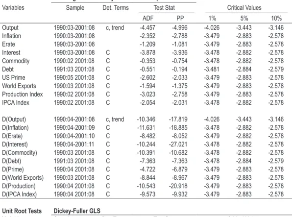
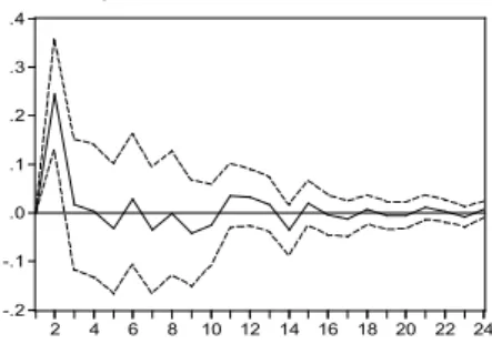
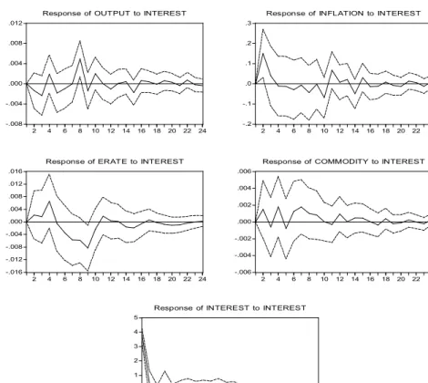
As the data set consists of monthly observations, first a VAR system with twelve lags of each variable, a constant and a deterministic trend was estimated.2_{The system is} stable as all inverse roots of the autoregressive polynomials are inside the unit circle. The dynamic responses of real economic activity and prices to an unanticipated increase in the nominal interest rate are shown in Figure 1. The solid lines indicate the point estimates of the dynamic response functions, while dashed lines represent a 95% confidence interval.

(9)

FIGuRE 1 – REsPonsEs oF outPut, InFlatIon and thE ExchanGE R atE to a MonEtaRy shock

-.008 -.004 .000 .004 .008 .012

2 4 6 8 10 12 14 16 18 20 22 24 Response of OUTPUT to INTEREST

-.3 -.2 -.1 .0 .1 .2 .3

2 4 6 8 10 12 14 16 18 20 22 24 Response of INFLATION to INTEREST

-.02 -.01 .00 .01 .02 .03

2 4 6 8 10 12 14 16 18 20 22 24 Response of ERATE to INTEREST

-2 -1 0 1 2 3 4 5

2 4 6 8 10 12 14 16 18 20 22 24 Response of INTEREST to INTEREST

Response to Cholesky One S.D. Innovations ± 2 S.E.

As one may see in the first graph, a tightening in the monetary policy has an imme-diate effect on economic activity, with the growth rate of real GDP reaching its lowest level in the second month following the shock. Real output tends to return to trend 12 months after the shock.

(10)

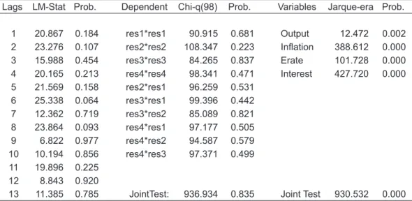
The regression residual tests were tested for autocorrelation, heteroscedasticity and normality (see Table 2). The results indicate absence of autocorrelation or heterosce-dastic autoregressive terms (ARCH), but indicate problems with normality.3

taBlE 2 – autocoRRElatIon, aRch tER Ms and noR M alIty tEsts oF thE REsIduals

Lags LM-Stat Prob. Dependent Chi-q(98) Prob. Variables Jarque-era Prob.

1 20.867 0.184 res1*res1 90.915 0.681 Output 12.472 0.002 2 23.276 0.107 res2*res2 108.347 0.223 Inlation 388.612 0.000 3 15.988 0.454 res3*res3 84.265 0.837 Erate 101.728 0.000 4 20.165 0.213 res4*res4 98.341 0.471 Interest 427.720 0.000 5 21.569 0.158 res2*res1 96.259 0.531 6 25.338 0.064 res3*res1 99.396 0.442 7 12.362 0.719 res3*res2 85.089 0.821 8 23.864 0.093 res4*res1 97.177 0.505 9 6.822 0.977 res4*res2 94.587 0.579 10 10.194 0.856 res4*res3 97.371 0.499

11 19.896 0.225

12 8.843 0.920

13 11.385 0.785 JointTest: 936.934 0.835 Joint Test 930.532 0.000

Note: High probability values indicate acceptance of the null of no autocorrelation, no heteroscedasticity and normality.

Information criteria were used to select a more appropriate specification for the num-ber of lags to be included in the endogenous variables in the VAR. The Akaike infor-mation criterion suggests a model with 2 lags, the more stringent Schwarz criterion suggests only 1 lag and a sequential likelihood ratio test selected 8 lags. The VAR system was re-estimated with the number of lags suggested.

Estimation with 1 or 2 lags resulted in models whose residuals were strongly autocor-related, heteroscedastic and non-gaussian, although the impulse response functions did not change in any substantial way.

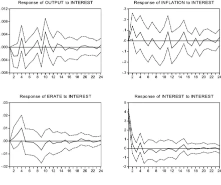
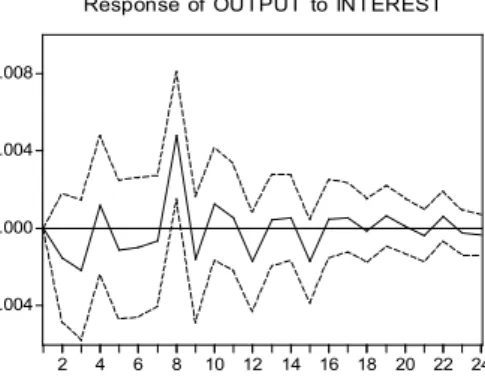
The VAR system with 8 lags delivered a more parsimonious model, with well behaved residuals in terms of autocorrelation and heteroscedasticity, although not in normality (see Table 3). The impulse functions are shown in Figure 2.

(11)

FIGuRE 2 – REsPonsEs oF outPut, InFlatIon and thE ExchanGE R atE to a MonEtaRy shock, laG lEnGth BasEd on InFoR M atIon cRItERIa

-.008 -.004 .000 .004 .008

2 4 6 8 10 12 14 16 18 20 22 24

Response of OUTPUT to INTEREST

-.2 -.1 .0 .1 .2 .3

2 4 6 8 10 12 14 16 18 20 22 24

Response of INFLATION to INTEREST

-.015 -.010 -.005 .000 .005 .010 .015 .020

2 4 6 8 10 12 14 16 18 20 22 24

Response of ERATE to INTEREST

-2 -1 0 1 2 3 4 5

2 4 6 8 10 12 14 16 18 20 22 24

Response of INTEREST to INTEREST

(12)

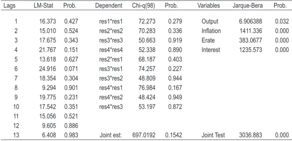
taBlE 3 – autocoRRElatIon, aRch tER Ms and noR M alIty tEsts oF thE REsIduals

Lags LM-Stat Prob. Dependent Chi-q(98) Prob. Variables Jarque-Bera Prob.

1 16.373 0.427 res1*res1 72.273 0.279 Output 6.906388 0.032

2 15.010 0.524 res2*res2 70.283 0.336 Inlation 1411.336 0.000

3 17.675 0.343 res3*res3 50.663 0.919 Erate 383.0677 0.000

4 21.767 0.151 res4*res4 52.338 0.890 Interest 1235.573 0.000

5 13.618 0.627 res2*res1 68.187 0.403

6 24.916 0.071 res3*res1 74.257 0.227

7 18.354 0.304 res3*res2 48.809 0.944

8 9.294 0.901 res4*res1 76.984 0.167

9 19.775 0.231 res4*res2 48.424 0.949

10 17.542 0.351 res4*res3 53.197 0.872

11 15.056 0.521

12 9.605 0.886

13 6.408 0.983 Joint est: 697.0192 0.1542 Joint Test 3036.883 0.000 Note: High probability values indicate acceptance of the null of no autocorrelation, no heteroscedasticity

and normality.

4. RoBustnEss analysIs and thE “PRIcE PuzzlE”

This section presents a robustness analysis for the results obtained with the bench-mark model by checking whether the qualitative results are sensitive to the period analyzed or to changing conditions in the international market. We also check whe-ther the qualitative results change when variables as excluded or included in the infor-mation set in an attempt to solve the “puzzles” presented by the benchmark model.

4.1 sample Period and Exclusion of the Exchange Rate

(13)

using two impulse dummies, D1= 1 in 1994:07, 0 otherwise and D2= 1 in 1999:01, 0 otherwise. The results are presented in Figure 4. Although the dummies are significant for some series, as one may observe, the pattern of the impulse response functions does not changed substantially4.

FIGuRE 4 – REsPonsEs oF outPut, InFlatIon and thE ExchanGE R atE to a MonEtaRy shock, contRollInG FoR PR IcE staBIlIzatIon and FloatInG ExchanGE REGIME

-.003 -.002 -.001 .000 .001 .002 .003 .004

-.08 -.04 .00 .04 .08 .12

-.006 -.004 -.002 .000 .002 .004 .006

2 4 6 8 10 12 14 16 18 20 22 24 Response of ERATE to INTEREST

-0.4 0.0 0.4 0.8 1.2 1.6 2.0

The robustness of the estimation can also be checked by eliminating some variables of the system and verifying whether the impulse response change substantially. During the sample period used for the analysis, the exchange rate regime has been changed. The price stabilization program of 1994 was based on a fixed exchange rate to the U.S. dollar. In January 1999, under a speculative attack, the Brazilian government liberalized the exchange rate, adopting a floating regime. In order to access the ro-bustness of the analysis conducted so far, it seems interesting to re-estimate the VAR excluding the exchange rate from the system, while maintaining the same identifica-tion assumpidentifica-tions. The results are shown in Figure 3.

(14)

FIGuR E 3 – systEM ExcludInG thE ExchanGE R atE FRoM thE InFoR M atIon sEt

-.008 -.004 .000 .004 .008

-.2 -.1 .0 .1 .2 .3 .4

-2 -1 0 1 2 3 4 5 6

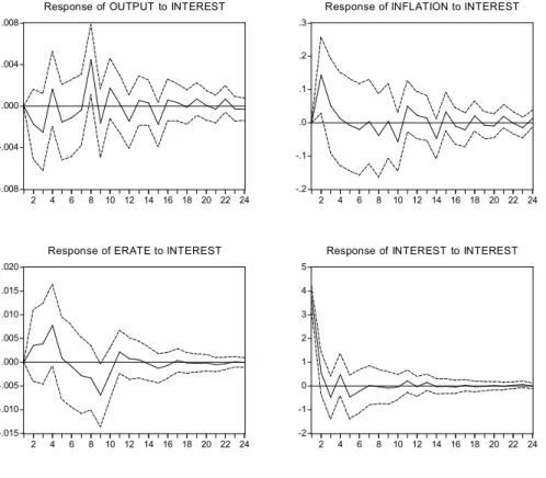
According to Figure 3, the response patterns of output and inflation to an unexpected policy shock are very similar to those portrayed in Figure 2. Output responds imme-diately to the shock and returns to its initial value 12 months later. As in Figure 2, here the inflation rate also rises after shock declining two periods after the shock.

4.2 controlling for International conditions

In order to take into account changing conditions in the international markets, an index for world exports and the U.S. Prime rate were included exogenously in the VAR system. The world exports’ index is used as a proxy for international economic activity, which may have a positive correlation with domestic output; the U.S. Prime rate may in turn affect the exchange rate, influence the domestic monetary policy and the interest rate.

(15)

significant at conventional levels. As before, residuals are uncorrelated, homoscedastic, but not normal. The impulse response functions patterns remain very similar to the ones previously reported (see Figure 5), showing that the inclusion of the exogenous variables does not change the results in any significant way.

FIGuRE 5 – REsPonsEs oF outPut, InFlatIon and thE ExchanGE R at E to a Mon Eta Ry shock, con t Rol l I nG FoR IntERnatIonal condItIons

-.004 .000 .004 .008

2 4 6 8 10 12 14 16 18 20 22 24

-.2 -.1 .0 .1 .2 .3

2 4 6 8 10 12 14 16 18 20 22 24

-.015 -.010 -.005 .000 .005 .010 .015 .020

2 4 6 8 10 12 14 16 18 20 22 24

-2 -1 0 1 2 3 4 5

2 4 6 8 10 12 14 16 18 20 22 24

4.3 the “Price Puzzle”

(16)

may appear to rise after a contractionary shock to the monetary policy because the analysis is based on a information set that does not include information on future inflation that is actually available to the authorities. For the American case, the inclusion of a commodity price index in the information set has often eliminated the “price puzzle” [Christiano et al (1996), Sims and Zha (1998)]. There, the inflation rate have been historically preceded by rises in commodity prices (Christiano et al, 1999). In addition, the evidence presented above show that besides the “puzzle” in prices, there is a “puzzle” in the exchange rate variable, a result that does not conform to theory or evidence (as shown by Eichenbaum and Evans,1995). The first question is then, does the inclusion of a commodity price index solve the “price puzzle” in the Brazilian case as it did for the American case? What about the “puzzle” in the exchange rate variable?

Data on commodity prices were collected from the International Financial Statistics Data Base, log transformed and tested for stationarity. As the unit root results (repor-ted in Table 1) indica(repor-ted the series to be first ordered integra(repor-ted, the variable entered in the analysis in first difference.

The VAR system was re-estimated with 8 lags of Output, Inf lation, Erate, Commodity and Interest, in this order, a constant and a deterministic time trend5. The impulse-response functions are reported in Figure 6.

As one may see from the second graph presented, the inclusion of a commodity price index does not solve the “price puzzle” or the “exchange rate puzzle” for Brazil. In fact, the responses to an unexpected change in the selic interest rate continues to be very similar to the ones previously reported. 6

5 First a 12 lag VAR system was estimated, resulting in very similar response-functions.

(17)

FIGuRE 6 – REsPonsE By outPut, InFlatIon and thE ExchanGE R atE to a MonEtaRy shock, coMModIty PRIcEs In thE InFoR M atIon sEt

-.008 -.004 .000 .004 .008 .012

2 4 6 8 10 12 14 16 18 20 22 24

-.2 -.1 .0 .1 .2 .3

2 4 6 8 10 12 14 16 18 20 22 24

-.016 -.012 -.008 -.004 .000 .004 .008 .012 .016

2 4 6 8 10 12 14 16 18 20 22 24

-.006 -.004 -.002 .000 .002 .004 .006

2 4 6 8 10 12 14 16 18 20 22 24

Response of COMMODITY to INTEREST

-2 -1 0 1 2 3 4 5

2 4 6 8 10 12 14 16 18 20 22 24

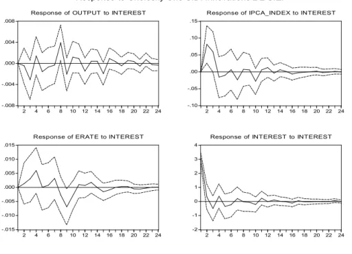
In the benchmark model, inflation was measured as a percentage change in the General Price Index, which is an average of wholesale prices, consumer price, and construction costs. output consisted of monthly observations of GDP, seasonally adjusted at constant prices of 1990. This series, published by the Instituto Brasileiro de Geografia e Estatística (IBGE), has been discontinued after 2001, an indication that there might measurement errors in this variable. The benchmark model was then also estimated with a consumer price index (IPCA) and with a proxy for output, an industrial production index (quantum)7_{. The impulse response functions, reported} in Figure 7 and Figure 8, have very similar patterns as the ones obtained by the ben-chmark model.

7 For comparability between the models, the variable IPca_ Index received the same treatment as

(18)

FIGuR E 7 – R EsPonsE By outPut, I nFl atIon (IPca) and thE ExchanGE R atE to a MonEtaRy shock

-.008 -.004 .000 .004 .008

2 4 6 8 10 12 14 16 18 20 22 24

-.10 -.05 .00 .05 .10 .15

2 4 6 8 10 12 14 16 18 20 22 24

Response of IPCA_INDEX to INTEREST -.015 -.010 -.005 .000 .005 .010 .015

2 4 6 8 10 12 14 16 18 20 22 24

Response of ERATE to INTEREST -2 -1 0 1 2 3 4

2 4 6 8 10 12 14 16 18 20 22 24

FIGuR E 8 – R EsPonsE By PRoductIon, I nFl atIon a nd thE ExchanGE R atE to a MonEtaRy shock

-.015 -.010 -.005 .000 .005 .010 .015

2 4 6 8 10 12 14 16 18 20 22 24

Response of PRODUCTION to INTEREST

-.2 -.1 .0 .1 .2 .3

2 4 6 8 10 12 14 16 18 20 22 24

Response of INFLATION to INTEREST -.016 -.012 -.008 -.004 .000 .004 .008 .012 .016

2 4 6 8 10 12 14 16 18 20 22 24

Response of ERATE to INTEREST -2 -1 0 1 2 3 4 5

2 4 6 8 10 12 14 16 18 20 22 24

(19)

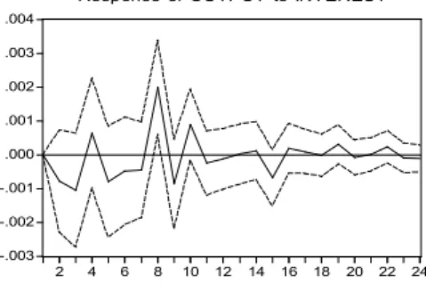
In Sargent and Wallace’s unpleasant monetarist arithmetic (Sargent and Wallace, 1981), fiscal variables may affect prices in an institutional setting where the monetary authority does not act independently from the fiscal authority and set its monetary targets in accordance to the fiscal budget. Given the relatively recent and reportedly low independence of the Brazilian central bank and the attention international inves-tors give to the fiscal stance of the government, a fiscal variable was included in the information set.8 Indeed, as Figure 9 indicates, the inclusion of the debt/GDP ratio in the government’s information set solves the “puzzle” for the exchange rate that, as expected, appreciates after a contractionary shock to the domestic interest rate. The “price puzzle” remains however, with Inflation declining only after the second period. debt increases immediately after the interest shock Given the relatively high participation of interest-indexed government securities and their short maturities, a shock to the selic rate has an immediate effect on the stock of government debt.

FIGuRE – REsPonsE By outPut, InFlatIon and thE ExchanGE R atE to a MonEtaRy shock, dEBt In thE InFoR M atIon sEt

-.008 -.004 .000 .004 .008 .012

2 4 6 8 10 12 14 16 18 20 22 24

-.3 -.2 -.1 .0 .1 .2 .3

2 4 6 8 10 12 14 16 18 20 22 24

-.02 -.01 .00 .01

2 4 6 8 10 12 14 16 18 20 22 24

-.012 -.008 -.004 .000 .004 .008 .012 .016

2 4 6 8 10 12 14 16 18 20 22 24

Response of DEBT to INTEREST

-3 -2 -1 0 1 2 3 4 5

2 4 6 8 10 12 14 16 18 20 22 24

(20)

5. volatIlIty analysIs

In this section, we analyze how the monetary shocks have contributed to the volati-lity of the economic variables included in the information set of the estimated model (Christiano et al., 1999). Tables 4 and 5 show the percentage of the variance of the k-period ahead forecast error in the variables of the benchmark model (output, Inflation, Erate, Interest) and the control model (output , Inflation, Erate, debt, Interest).

In the benchmark model, the interest shock is relatively important for the volatility of the growth rate of output, significantly accounting for 8.0%, 9.1% and 9.7% of the variance of the 8, 12 and 24 period-ahead forecast error variance, respectively. For inflation and the exchange rate, the interest shock significantly accounts for 6.0% of the variance of the 18 month-ahead forecast error variance in inflation and 7.8% of the variance of the 12 month-ahead forecast error in the exchange rate. As expected given the ordered of the variables in the var system, the monetary policy shock has an important impact on the volatility of the interest rate, significantly accounting for more than 60% of the forecast error variance throughout the period analyzed.

taBlE 4 – PERcEnt oF k-PERIod ahEad FoREcast ERRoR vaRIancE duE to IntEREst shock, BEnchM aRk ModEl

2 4 8 12 18 24 36

Output _0.9 _3.3 _8.0 _9.1 _9.5 _9.7 _9.7

(0.577) (0.985) (1.862) (1.927) (1.932) (1.873) (1.784)

Inla

-tion 4.0 4.4 4.4 5.4 6.0 6.1 6.2

(1.317) (1.407) (1.335) (1.517) (1.666) (1.606) (1.580)

Erate _0.7 _4.4 _5.2 _7.8 _7.9 _7.9 _7.9

(0.391) (1.053) (1.179) (1.638) (1.586) (1.545) (1.497)

Inter-est 69.6 65.3 64.6 64.0 63.8 63.7 63.7

(10.403) (10.031) (9.791) (10.044) (9.985) (9.777) (9.136)

Ordering: OUTPUT INFLATION ERATE INTEREST; t-values calculated based on Monte Carlo es-timated standard errors in parenthesis; Significance levels: t = 1.645 (10%), t = 1.96 (5%), t = 2.326 (1%).

(21)

on the volatility of these variables.9 On the other hand, the monetary shock has an important and statistically significant impact on the volatility of the exchange rate and the debt/GDP ratio. The shock accounts for 11.9% and 12.4% of the 12 and 24 period-ahead forecast error variance of the exchange rate, respectively. The shock has also an important and significant impact on the volatility of the debt/GDP ratio, accounting for 20.2% of the 24-period ahead forecast error variance.

taBlE 5 – PERcEnt oF k-PERIod ahEad FoREcast ERRoR vaRIancE duE to IntEREst shock, contRol ModEl

2 4 8 12 18 24 36

Output 2.0 7.1 9.9 11.4 11.6 11.9 12.0

(0.735) (1.398) (1.432) (0.819) (1.552) (1.506) (1.332)

Inlation 1.4 2.3 3.3 5.4 8.2 8.5 8.6

(0.192) (0.793) (0.850) (1.022) (1.291) (1.229) (1.116)

Erate 0.0 1.1 7.2 11.9 12.4 12.4 12.5

(0.000) (0.373) (0.573) (1.882) (1.795) (1.628) (1.408)

Debt 11.0 19.6 20.8 19.7 20.2 20.2 20.2

(1.810) (2.691) (3.045) (2.882) (3.008) (2.975) (2.611)

Interest 73.8 66.7 65.3 64.5 64.0 63.9 63.8

(11.589) (9.608) (9.526) (9.228) (8.606) (8.023) (7.334)

Ordering: OUTPUT INFLATION ERATE DEBT INTEREST; t-values calculated based on Monte Carlo estimated standard errors in parenthesis; t = 1.645 (10%), t = 1.96 (5%), t = 2.326 (1%).

In both models, the benchmark and the control model, the variation of the forecast errors due to the policy shock are limited however, indicating that interest rate shocks have not been the most important independent source of volatility for these macro-economic variables.

6. FInal REMaRks

This article has analyzed the transmission mechanism of the Brazilian monetary policy during the 1990s using a standard specification of the information set of the monetary authorities, where the current level of economic activity, the inflation rate and the exchange rate are taken into account when setting its policy variable, the baseline interest rate. The results have indicated that a tightening in the monetary

(22)

policy immediately reduces economic activity, but only affects prices and the exchan-ge rate with a temporal lag. The robustness analysis conducted supports these main results.

The standard specification of the information set used led to the implication that a tightening in the monetary policy results in a initial rise in domestic prices. This effect, not supported by conventional theory of the monetary policy, has been com-monly reported in the empirical literature on the monetary transmission mechanism using vector-autoregressions and became known as the “price puzzle” (Eichenbaum, 1992). Moreover, the benchmark model indicates an “exchange rate puzzle”, as a contractionary shock leads to a depreciation of the domestic currency relative to trend. These “puzzles” may reflect the choice of variables in the governments information set. For the American case, the inclusion of a commodity price index in the informa-tion set has often eliminated the “price puzzle”. For Brazil, the results have indicated that the commodity price index or other variables, such as oil prices, have not solved the “price puzzle”. The “puzzle” in the exchange rate variable is removed, however, when the debt/GDP ratio is endogenously included in the model, indicating that fiscal variables have an important role in the government’s information set.

REFEREncEs

Ball, L. Time-consistent policy and persistent changes in inflation. Journal of Monetary

Economics, v.36, n.2, p. 329-350, 1995.

Barbosa, F. H.; Portugal, P. A. A transmissão da política monetária no Brasil: o canal

da taxa de juros.Rio de Janeiro: FGV, 2002. (Mimeografado)

Barro, R. Unanticipated money growth and unemployment in the United States. american Economic Review, v. 67, n.2, p. 101-115, 1977.

Barth, M.; Ramey, V. The cost channel of monetary transmission. nBER Working

Paper No. 7675, 2000.

Bernanke, B.; Blinder, A. The federal funds rate and the channels of monetary

trans-mission. american Economic Review, v.82, n.3, p. 901-921, 1992.

Bernanke, B.; Gertler, M. Inside the black box: the credit channel of monetary policy

transmission. Journal of Economic Perspective, v.9, n.4, p. 27-48, 1995.

Bernanke, B.; Mihov, I. Measuring monetary policy. nBER Working Paper 5145,

1995.

Blanchard, O. Why does money affect output? A survey. In: Friedman, B.; Hahn,

F. (eds.). handbook of Monetary Economics, v. 2. Amsterdam: North Holland,

(23)

Chari, V.; Christiano, L.; Eichenbaum, M. Expectation traps and discretion. Journal of Economic theory, v.81, n.2, p. 462-492, 1998.

Christiano, L.; Eichenbaum, M.; Evans, C. L. Identification and the effects of

monetary policy shocks. Federal Reserve Bank of chicago, Working Paper94-7,

1994.

________ . The effects of monetary policy shocks: evidence from the flow of funds. Review of Economics and statistics, v.78, n.1, p.16-34, 1996.

_________. Monetary policy shocks: what have we learned and to what end? In:

Taylor, J.; Woodford, M. (eds.). handbook of Macroeconomics, v. 1A. Amsterdam:

North Holland, 1999.

Cochrane, J. H. Shocks. carnegie-Rochester conference series on Public Policy 41,

p.1-56, 1994.

_________. What do the VARs mean? Measuring the output effects of monetary

policy. Journal of Monetary Economics, v. 41, n. 2, p. 277-300, 1998.

Cook, T.; Hahn, T. The effect of changes in the Federal Funds rate target on market

in-terest rates in the 1970s. Journal of Monetary Economics, 24, p. 331-51, 1989.

Eichenbaum, M. Comment on interpreting the macroeconomic time series facts:

the effects of monetary policy. European Economic Review, v. 36, n.5,

p.1001-1011, 1992.

Eichenbaum, M.; Evans, C. Some empirical evidence on the effects of shocks to

monetary policy on exchange rates. the Quarterly Journal of Economics, v.110,

n. 4, p.975-1009, 1995.

Friedman, M.; Schwartz, A. a monetary history of the united states, 1867-160.

Prin-ceton, NJ: Princeton University Press, 1963.

Hayashi, F. Econometrics. Princeton, NJ: Princeton University Press, 2000.

Mendonça, H. F. Mecanismos de transmissão monetária e a determinação da taxa de

juros: uma aplicação da regra de Taylor ao caso brasileiro. Economia e sociedade

16, 2001.

Minella, A. Monetary policy and inflation in Brazil. Working Paperseries 33, Banco

Central do Brasil, 2001.

Peersman, G.; F. Smets, F. The monetary transmission mechanism in the Euro area:

more evidence from VAR analysis. European central Bank, Working Paper 91,

2001.

Reichenstein, W. The impact of money on short-term interest rates. Economic Inquiry,

v. 25, n.11, p. 67-82, 1987.

Romer, C.; Romer, D. Does monetary policy matter? A new test in the spirit of

(24)

Sargent, T.; Wallace, N. Some unpleasant monetarist arithmetic. In: Preston, M. the rational expectations revolution: readings from the front line, 1994. Cambridge: The MIT Press, 1981.

Sims, C. Interpreting the macroeconomic time series facts: the effects of monetary

policy. European Economic Review, v. 36, n.5, p.975-1000, 1992.

Sims, C.; Zha, T. Does monetary policy generate recessions? Working Paper 8-12,

Federal Reserve Bank of Atlanta, 1998.

aPPEndIx

The raw data set was obtained from IPEA (site: www.ipea.gov.br).The following variables were downloaded:

Inflação: IGP:DI %

Taxa de câmbio - R$ / US$ - comercial - venda - média - Mensal - R$

IPC - índice (média 1995 = 100) - EUA - Mensal

IGP - índice (Dec95=100) - Brasil - Mensal

PIB - preços de mercado - índice encadeado (média 1990 = 100) - Mensal - Brasil

Taxa de juros - Over / Selic (% a.m.) - Mensal

Exportações Mundiais- índice (média 1995=100)

Prime - taxa de juros EUA, mensal (IFS12)

IPCA - geral - índice (dez. 1993 = 100) - Mensal - IBGE/SNIPC - Precos12_IPCA12

Produção industrial - indústria geral - quantum - índice (média 1991 = 100) - Mensal - BRASIL

Debt – dívida interna – setor público – líquida- mensal- (%PIB) – BCB Boletim/F.Públ. – Bm12_DINSPY12

Data on commodity prices and oil prices were obtained from the Financial International Statistic Data Base:

Commodity Price Index, baseyear 1995, series code: 00176AXDZF.