Which strategy for inbound tourism in Portugal? Contribution to a product life cycle model

E S T U D O S I I

Cidadania, Instituições e Património Economia e Desenvolvimento Regional Finanças e Contabilidade Gestão e Apoio à Decisão Modelos Aplicados à Economia e à Gestão

Faculdade de Economia da Universidade do Algarve

2005

F

COMISSÃO EDITORIAL

António Covas Carlos Cândido Duarte Trigueiros Efigénio da Luz Rebelo João Albino da Silva João Guerreiro

Paulo M.M. Rodrigues Rui Nunes

_______________________________________________________________________

FICHA TÉCNICA

Faculdade de Economia da Universidade do Algarve

Campus de Gambelas, 8005-139 Faro Tel. 289817571 Fax. 289815937 E-mail: ccfeua@ualg.pt

Website: www.ualg.pt/feua

Título

Estudos II - Faculdade de Economia da Universidade do Algarve

Autor

Vários

Editor

Faculdade de Economia da Universidade do Algarve Morada: Campus de Gambelas

Localidade: FARO Código Postal: 8005-139

Capa e Design Gráfico

Susy A. Rodrigues

Compilação, Revisão de Formatação e Paginação

Lídia Rodrigues

Fotolitos e Impressão

Grafica Comercial – Loulé

ISBN

972-99397-1-3 Data: 26-08-2005

Depósito Legal

218279/04

Which strategy for inbound tourism in Portugal?

Contribution to a Product Life Cycle Model

Eduardo Casais

Faculdade de Economia, Universidade do Algarve

Resumo

O turismo internacional vale cerca de 5% do PIB na economia portuguesa. Infelizmente, nos últimos anos, os fluxos de turismo para Portugal acusam uma desaceleração em volume e em valor. Tendo em conta os prazos dilatados que medeiam entre as etapas da decisão e da exploração nesta indústria, a capacidade de prever e antecipar as tendências futuras toma particular relevo para a tomada atempada e informada de decisões estratégicas.

O PLC (product life cycle ou ciclo de vida do produto) é utilizado em marketing, a fim de analisar a evolução da procura ao longo do tempo e tirar ilações para a orientação futura do negócio.

Com vista a modelizar o PLC do turismo em Portugal, recorremos à dinâmica de sistemas, procurando identificar a estrutura e compreender o comportamento da procura de turismo no horizonte de 2004 até 2030. Por meio de simulações e da análise de sensibilidade do sistema, procurámos isolar as variáveis que mais influem sobre o volume de entradas de turistas e o valor das receitas produzidas.

O comportamento do modelo sugere que há vantagem a médio e longo prazo em romper com a política tradicional de corrida atrás do volume, e em enveredar por uma orientação que favoreça declaradamente a busca de clientes mais valiosos, a oferta de produtos turísticos de gama alta e o desenvolvimento de programas de marketing relacional tendentes a alongar a duração de vida média do turista (tourist lifetime).

Esta viragem estratégica promete retardar significativamente o ponto de inflexão entre a etapa de maturidade e o declínio do turismo em Portugal e produzir receitas sensivelmente mais abundantes durante um lapso de tempo mais dilatado.

Palavras-chave: Turismo, Ciclo de Vida do Produto (PLC), Modelação,

Simulação, Análise de Sensibilidade, Segmentação, Marketing Relacional.

Abstract

In recent years, inbound international tourism in Portugal, as measured in arrivals and receipts, has shown a decelerating trend. Taking into account that tourism business weighs 5% of GDP in the Portuguese economy, and that there are huge delays in moving from decision to implementation in this industry, it would be advantageous to assess at what stage tourism currently is, and what is likely to come after, so that tourism officials and executives could make proper and timely policy decisions.

The PLC (Product Life Cycle) marketing tool is dedicated to performing this function. In applying PLC to the analysis of Portugal’s inbound tourism, a causal model has been built. Two scenarios, a low end and a high end one, were modelled using the same basic structure.

By simulating the model and performing sensitivity analysis of key variables, it appears that a change in policy could prove quite beneficial in the medium and long run. The segmentation of the potential market, the shift from a business-as-usual posture towards an emphasis on high end tourists and high grade product, as well as focusing on effective customer relationship programmes with a view to extend the tourist lifecycle, promise to delay significantly the turning point between the mature and the decline stages of the PLC, and to provide significantly higher receipts during an extended lifetime period.

Keywords: tourism, PLC (product life cycle), modelling, simulation, sensitivity

analysis, segmentation, customer relationship.

1. The issue

Tourism1 _{is unquestionably a major economic contributor, both from the}

worldwide and the Portuguese vantage points. Understood as both international tourism and international fare receipts, it represented in 2002 (WTO 2003) approximately 7% of worldwide exports of goods and services, occupying the fourth position in the ranking after exports of chemicals, automotive products and fuels. When considering service exports exclusively, the share of tourism exports increases to nearly 30%. Since fare receipts only account for 1.3%, tourism receipts rise to 6% of worldwide exports.

As far as Portugal is concerned, tourism receipts weigh comparably even more. According to WTO estimates of Portuguese tourism receipts for 2003 (WTO 2004), the latter amounted to close to 5% of the GDP or more than 7% of Services, and a sizable 16% of Exports (FOB), all at current prices (INE 2005).

At first glance, the situation looks just fine. However, an issue lurks around the corner: its term. Will the blessings of tourism last a long enough period for the required investments in capacity to pay back? What are the positive feedback loops of the growing tourism industry? Are there any negative feedbacks? How will both evolve along the years, and how will they balance out?

2. The PLC (product life cycle) concept

As the old French saying goes, “tout passe, tout casse, tout lasse”, in other words everything breaks away and nothing lasts forever. This plain fact of life was introduced in strategic marketing decades ago with the concept of PLC (product life cycle) (Levitt 1965). By PLC, we understand the result of multiple supply and demand forces translating into a sequential path that products follow from their embryonic, through the maturing, down to the declining stage, in terms of volume of demand and revenue. This evolution has deep impact on the product’s sales and profits over its lifetime (Kotler 1993).

“That products pass through various stages between life and death is hard to deny […] Thus the concept of a product life cycle would appear to be an essential tool for understanding product strategies. Indeed this is true, but only if the position of the product and the duration of the cycle can be determined.” (Day 1975). An attempt to provide for this demand consists of identifying common product life cycle curves, e.g. the classical, growth-decline-plateau, innovative-maturity, and cycle-recycle curves (Swan and Rink 1980). It is self-evident that, should one be able to predict the evolution of sales, revenues and costs along a timeline, decisions regarding investment, capacity building, promotion, targeting, product changes, distribution, and prices could become far easier to compute and develop.

Unfortunately, timelines are tricky, and there are no known fail safe models to predict the course of the future. We may have to conclude with Simon (1990) that “we must give up prediction as the primary goal of modeling”, especially as regards models of large, complex and dynamic systems, of which tourism is an instance. Instead, we should concern ourselves with examining the future consequences of today’s decisions. Our aim becomes the building and running of models to understand the consequences of taking one decision or another. “Our decisions today require us to know our goals, but not the exact path along which we will reach them” (Simon ibidem).

The PLC is such a model. It adopts a normative approach to product strategies based on assumptions concerning the features or characteristics of each stage. Hence, the decision maker must “also consider forces relating to the product, the market and the competitive environment” (Boyd and Walker 2000).

3. PLC as a procedural tool

In many markets, competitive pressures, technology and product developments, combined with apparently erratic movements of exogenous variables all converge towards reducing the duration of economic life cycles to a fraction of the product physical life expectancy. In some cases, for example in some telecommunications markets, not only the expected economic life cycle may be a low 40% of the product physical life cycle, but

furthermore the actually observed economic life cycle varies from 44% to a meagre 18% of the projected economic life cycle (Barreca 1999).

Should such a pattern manifest itself in the tourism industry, the quality of the decisions by the concerned entrepreneurs and executives could be significantly reduced. The risk would be immense that the results of the said decisions be jeopardised. Calculations of rates of return and pay-back periods would become extremely hazardous.

Consider, for instance, the development of a new tourist resort. The elapsed time between the first step of the decision stage (planning, financing, regulatory requirements) and the action stage (building, operating), in other words from the moment the process starts to the moment when the first carloads of tourists check in, may be of 5 to 10 years. For business planning, this is a hard lag time during which only cash outflows occur.

Although the resort may last physically for 50 years or more, the infrastructure is expected to perform at a profitable level of capacity for not more than a decade without fundamental upgrades. For business purposes, the physical life cycle of this specific product is therefore estimated at 10 years. To calculate the pay-back period, one assumes that the economic life cycle equals the physical one, i.e. 10 years.

Now, by reasons such as those quoted by the WTO 2_{, let us assume that the}

economic life cycle is reduced to 50% of the physical one, causing the pay-back period to be reduced to 5 years instead of the original 10 years. Assuming further that the actual economic life cycle is just 50% of the planned one, the rate of return will have to be adjusted to a catastrophic pay-back period of only 2.5 years.

Foreseeing these developments 5 years ahead of time (the incompressible initial lag time estimate) can be an insurmountable task. In fact, trying to overcome the hurdle by commissioning more research only compounds the problem, since this would cause further delays. In such a deadlock, the options are reduced to either reasonably decide to stay out and not to compete for a share of the market, or alternatively make a risky decision based on scant information and plethoric faith.

In such a situation of uncertainty, suggests Simon (1976), it is preferable to stand for a good decision-making procedure (“procedural rationality”), rather than to look for the optimal result (“substantive rationality”). A good procedure, which can dispense with lengthy search for more information, offers the superiority of an instantly applicable decision over a theoretically optimal decision (Sapir 2003). In our hypothetical example, the advantage of a procedure that provides an effective base for making decisions, without requiring a time-consuming and hazardous research of otherwise unreliable information, simply imposes itself. PLC helpfully offers such a rational procedure.

4. Forecasting demand and sales with a logistic curve

The forecast of demand and sales for the tourism product 3 _{throughout its entire life} cycle is critical to schedule and plan supply, and build tourism as well as promotional and distribution capacity. The exercise entails not only the forecast of demand volume and sales revenue at a single point in time, say of the mature product, but also longitudinally, embracing the transitional phases from the introduction until the phase out.

Elementary forecasting techniques, for instance moving averages and exponential smoothing, do not perform very effectively (Armstrong and Brodie 1999). A number of marketing professionals, including the best known consulting firms, and marketing scholars, although acknowledging that the life cycle curve varies significantly between and within industries, claim that it can be better described by an S-shaped curve. Many growth phenomena, from epidemics to advertising awareness, to the diffusion of innovation, to the rise and fall of the “new economy” (Modis 1992, Modis 2003, Mahajan et al 2000, Bass 1969, Rogers 1995, Oliva et al 2002) are characterised by an S-shaped curve representing sequential periods with different growth behaviours. First, as it is typical of exponential growth, there is a period of initial inertia, during which growth is slow. Thereafter comes a period of increasing returns, during which growth accelerates exponentially. But exponential growth cannot go for ever; there is a ceiling that constrains the possible growth. This limit imposes an inflection point after which growth decelerates. Eventually, the curve moves towards equilibrium, and growth tends asymptotically to zero.

A number of instruments are used to model this dynamic pattern. The family of sigmoid functions, also known as logistic curves, including the Verhulst logistic curve, Richard’s curve, Pearl-Reed growth curve, Fisher-Prey transform, Gompertz curve, or the Bass model, respond to the concept of the S-shaped curve. I propose to explore the usefulness of the logistic curve to model the PLC of tourism.

The logistic curve requires three parameters. First, M is the limit, in this case the total number of Potential ITA (international tourist arrivals4_{). Secondly, n}

0 is the initial

value at time t = 0, in our case the first data point of the Actual ITA series. Thirdly, the constant c, corresponding to the rate of conversion of Potential ITA into Actual ITA.

3 _{Following the WTO (1995), the tourism product comprises:}

“Accommodation services”, “Food-and beverage-serving services”, “Passenger transport services”, “Travel agency, tour operator and tourist guide services”, “Cultural services”, “Recreation and other entertainment services”, “Miscellaneous tourism services.”

4 _{ITA (International Tourist Arrivals) (WTO 1995) is the most common unit of measure used to quantify the volume}

of International Tourism for statistical purposes. It refers exclusively to tourists (overnight visitors). It also refers to the number of arrivals and not to the number of persons. The same person who makes several trips to a given country during a given period will be counted as a new arrival each time, as well as a person who travels through several countries on one trip is counted as a new arrival each time.

The model assumes that for a period ∆t, the sales effort converts c∆t Potential ITA into Actual ITA. Assuming that at time t there are n(t) Actual ITA, the latter’s number will be

n(t+∆t)= n(t) c ∆t (1)

Equation (1) can be converted to the differential equation

) ( ) ( ) ( t n M t n M c dt t dn × − × = (2) The equivalent integral equation is

τ τ τ _{n d} M n M c n t n t ) ( ) ( ) ( 0 0 × − × + =

_∫

t c e n n M M t n ∗ −       − + = 0 0 1 ) ( , t ≥ 0 (4)

Using WTO statistics for the period 1950-2002, I developed the logistic curve for World and Europe ITA. The used parameters are:

• M : World = 1.56 billion; Europe = 717 million, as given by WTO forecasts for 2020 (WTO 2001).

• n0 : World = 25.3 million; Europe = 16.8 million, as given by WTO for 1950

(Source: International Tourist Arrivals 1950-2002, World Tourism Organization, data as collected by WTO September 2003).

• c : World = 0.09084; Europe = 0.092630, calculated by the least squares method based on the average growth rates between 1950 and 1975 (same source).

I assume that, if the S-curve model is effective, it should be able to reasonably predict the actual evolution until and beyond 1975. Although this has been verified in a number of other industries I am familiar with, in the case of tourism it is unfortunately far from being true.

Figure 1: Logistic curves of International Tourist Arrivals compared with actual values. 0 500 1000 1500 2000 2500 3000 195019521954195619581960196219641966196819701972197419761978198019821984198619881990199219941996199820002002 IT A M il li o

n World - logistic curve

Europe - logistic curve World - actual Europe - actual

Figure 1 shows the logistic curves for World and Europe ITA parameterised as per the above values, as well as the actual values provided by the WTO (same source). Not surprisingly, the fit is good until 1975, but quite below expectations thereafter. The steep take-off predicted by the logistic curve around 1984 is not validated by the actual data. Further attempts using different statistical series and other sigmoid functions produced equally disappointing results. It is useless to speculate about the reasons. The sensible conclusion to draw is that, in the absence of other data allowing for a more precise and reliable parameterisation, one should not waste more time with a method that is patently unable to represent the life cycle of tourist arrivals.

5. System dynamics model

Since time-series models do not meet requirements, the alternative chosen is to use a causal model instead. I choose system dynamics (SD) modelling, as this not only incorporates explicit causal assumptions, but also provides a wealth of simulation functionalities capable of supporting the decision maker in designing alternative policies and structures, educate and debate, and implement changes in policies and structure (Forrester 1994). From this viewpoint, SD compares advantageously with other modelling approaches or techniques, such as optimisation or econometric models (Sterman 1991), as summarised in Table 1.

Table 1: Comparative evaluation of SD, optimisation and econometric models.

Models Advantages Limitations

SD (System dynamics) models

Descriptive: clarifies what would happen in a given situation.

Little guidance exists for

converting a real-life situation into a model.

Easily incorporate qualitative

(“soft”) variables, feedback

effects, nonlinearities, and

delays.

Decision rules used by the people

in the system cannot be

determined from aggregate

statistical data, but require first hand investigation.

Easily perform “what if”

sensitivity analysis.

Difficult to define the model boundaries: which factors are genuinely exogenous, which ones are endogenous?

Optimisation models

Yield the best solution given the assumptions of the model: the goals to be met (objective function), the choices to be made (decision variables), and the constraints to be satisfied.

The objective function embodies values and preferences, but which values, whose preferences?

Predominantly assume that the relationships in the system are linear, mostly ignore feedback effects, and neglect delays. Econometric

models

One of the most widely used formal modelling techniques.

Draw on economic theory, with questionable assumptions (such

as optimisation; perfect

information; exclusive profit or utility maximisation behaviours; and equilibrium) to build the relationships in the model.

Linearity and static thinking prevail; state transitions are assumed to be stable and smooth. Estimation is made by statistical regression, which cannot prove whether or not a relationship is causal.

In building the SD model, I followed the recommended (Sterman 2000) methodological steps.

1. Problem Area

1.1. International inbound tourism has been identified as a major contributor to the Portuguese economy. Policy makers, tourism officials and entrepreneurs have made efforts to give momentum to, and grow the inflow of international tourists. 1.2. However, analysts have pointed out a targeting dilemma. Should the tourism

sector focus on high volume and low price tourist segments? Or should it alternatively focus on low volume and high price segments? Each one has pros and cons. This is a classic strategic marketing issue. Both differentiation and low-price strategies carry a risk, but this is nothing compared with the risk of getting “stuck in the middle” by trying to be everything for everybody (Porter 1985). 2. Purpose of the model

2.1. To estimate the evolution of international tourist arrivals (ITA) and international tourism receipts (ITR 5_{), i.e. the fundamental components of the tourism PLC,}

until 2030, under two different sets of assumptions:

2.1.1. First, the Base Line (BL) (projection of perceived current conditions).

2.1.2. Second, the High End (HE) focus: with emphasis on catering for high-value tourists.

2.2. The model does not attempt to represent the whole tourism business model, leaving out variables such as:

2.2.1. National tourists.

2.2.2. Costs, margins, rates of return, return on investment or lead time to build capacity.

2.2.3. The internal and external agents involved.

2.2.4. The specific processes by which tourism business is carried out.

2.3. The geographic reach of the model is Portugal, with a view to benefit from comparable statistical series available from WTO for the World, Europe and individual countries. Nevertheless, at this stage, it is a rather abstract Portugal. Not only some parameters are judgementally estimated from partial data on Algarve, but also no effort has been made to differentiate amongst the various Portuguese destinations.

5 _{ITR (International Tourism Receipts) (WTO 1995) “are the receipts earned by a destination country from inbound}

tourism and cover all tourism receipts resulting from expenditure made by visitors from abroad, on for instance lodging, food and drinks, fuel, transport in the country, entertainment, shopping, etc. This concept includes receipts generated by overnight as well as by same-day trips, which can be substantial, as will be the case with countries where a lot of shopping for goods and services takes place by visitors from neighbouring countries. It excludes, however, the receipts related to international transport contracted by residents of other countries (for instance ticket receipts from foreigners travelling with a national company).”

3. Model audience

3.1. The information generated is ultimately intended for everyone (professionals, scholars, tourism officials and executives) involved in developing and analysing marketing strategies for inbound international tourism.

4. Key model boundary components

Endogenous Components Exogenous Components Potential tourist arrivals (Stock) Tourist population Tourist arrivals (Stock) Linear capacity Receipts per tourist (Stock) Conversion fraction Tourist acquisition (Flow) Initial tourist receipts Tourist quit (Flow) Growth fraction of receipts Growth of tourist receipts (Flow)

5. Assumptions or constraints for the Base Line model

Variable Estimate Assumption

Total ITA available World ITA, 700 million in 2003, projected

to grow by 4.1% yearly (WTO 2001, 2003). This variable sets the limit to tourism demand.

[1]

Potential ITA 10% of [1], or roughly 50% of expected

market share of the Mediterranean region in 2020 (WTO 2001). The ceiling could also be derived from the ratio of ITA relative to the country population, the highest in Europe (excluding the special case of Andorra, No.1 worldwide with a ratio of 50) being Austria (ratio of 2.3), Portugal having a ratio of 1.2 (WTO 2003).

[2]

Conversion fraction By assumption, distribution channel

programmes yield 10%, and promotion (advertising, e-marketing, fairs, etc.) 5%.

[3]

Initial ITA LowEnd Initial ITA HighEnd

ITA in Portugal reached 11.7 million in 2003. To discriminate between low and high end tourists, I used the rate of bed occupancy by foreigners in 5-star hotels

represent therefore an 85% fraction of the 11.7 million.

Linear capacity Currently, Portugal is predominantly a 3S

(Sun-Sand-Sea) destination. I therefore used the linear length of Algarve beaches as the basis for density estimates. Since there are 45 km of beaches in Algarve (source: PROT Algarve – Opções para os Algarvios, CCRA April 1990), I estimate the total Portuguese linear capacity at slightly more than twice that value, i.e. 100 km. This variable sets the limit to tourism product supply.

[5]

Normal tourist density I assume that 120% of the actual ITA for

2003 (11.7 million) could “normally” be accommodated by the existing linear capacity. In order to normalise the density, I further assume that tourists arrive from May to October (6*30 = 180 days) and they go to the beach either in the morning, or in the afternoon (2 shifts). In other words, there are supposedly 180*2 = 360 “slots” for international tourists.

Taking into account the 15% - 85% split (see [4]) between high end and low end tourists, I estimate normal density at 0.33 t/m (tourist per linear meter) or 3 linear meters per tourist for low end tourists.

It is assumed that high end tourists have more demanding requirements, leading to a normal density of 0.1 t/m (or 10 linear meters per tourist).

[6] Lifetime LE Tourist Lifetime HE Tourist LE guess-estimated at 2 years. HE guess-estimated at 3.5 years. [7] LE Quit HE Quit

The number of tourists that cease to be tourists in Portugal equals the number of total tourists divided by the corresponding lifetime. This flow may be increased or decreased by the multiplier.

LE Quit Multiplier HE Quit Multiplier

If the relative density (calculated as the tourist density divided by the normal tourist density) goes below a certain value, a number of low end tourists may be induced to extend their lifetime by coming a third year. Conversely, if it goes above a given value, some will not come the second time, shortening therefore the average lifetime. This is a non-linear function given by a specific Lookup table.

The same behaviour applies to high end tourists, except for the timing and slope of the function in the corresponding Lookup table.

[9]

Initial LE Receipts Initial HE Receipts

The average receipts per tourist amount to EUR 524 in 2003 (WTO 2003, 2004). Assuming that high end tourists generate receipts twofold bigger than low end tourists, and given the split between the two categories, the average initial receipts are 912 per HE tourist, and 456 per LE tourist.

[10]

Growth Fraction LE Growth Fraction HE

Receipts per tourist grew at an average rate of 3.19% between 1990 and 2003 (WTO same sources). In 2003, this rate occupies the 25th percentile in the array of growth rates for nine Mediterranean countries (from Croatia with 12.8% to Tunisia with 1.3%). I assume that policy makers will endeavour to raise the average HE growth rate to reach 5.25%, (equivalent to the 67th percentile in the 2003 ranking) by 2030. However, as regards LE growth rate, the current growth rate of 3.19% remains unaltered, for reasons of assumed competitive policies based on price-elasticity.

6. Dynamic hypothesis

6.1. Building capacity and sustaining the marketing promotion effort create a positive feedback loop, causing the number of ITA to grow exponentially initially. 6.2. However, there is a limit to growth set ultimately by (a) the potential ITA (a

fraction of the total number of international tourists available), and in the nearer future by (b) the tourist lifetime, on one hand, and (c) the maximum linear capacity of the destination on the other hand. These create a negative feedback loop, causing an asymptotic decay to equilibrium.

6.3. The combination of the positive and negative feedbacks drives the eventual decrease of ITA and ITR, the dynamics of which follow a growth-and-decay curve.

6.4. Causal-loop diagram

Figure 2 illustrates the causal-loop diagram representation of the basic mechanisms driving the ITA behaviours.

Figure 2: Causal-loop diagram of international tourist arrivals.

LE International Tourists HE International Tourists International Tourists Available tourist density + + + + Capacity Demand exceeds capacity Gap HE Expectations + -+ -+

-6. The SD Base Line Model

The Base Line model is a stock-and-flow structure incorporating the assumptions stated above. All systems that evolve throughout a period of time can be represented by using stocks (or levels), and flows (or rates). Stocks are accumulations. For instance, arrivals of tourists change over time, moving from an initial to a different level. The changing does not occur instantaneously, but gradually. Flows cause the changing, by increasing or decreasing stocks every unit of time. In this model, the stock of accumulated ITA increases as newly acquired ITA flow in each unit of time. Simultaneously, the stock decreases as a fraction of ITA quit each unit of time.

Mathematically, the modelling language is equivalent to:

∫

(stocks aux data const g flowst = t t t ₍₂₎ ) , , ,

(stocks aux data const f aux_t = _{t t t (3)} ) , , , ( _{0 0 0}

0 h stocks aux data const

stocks = ₍₄₎

Equation (1) represents the evolution of the system over time, at a rate represented by (2). Equation (3) represents the intermediate results required to calculate the rates, and (4) the initialisation of the system. In these equations, g, f, and h are arbitrary, nonlinear, possibly time varying, vector-valued functions.

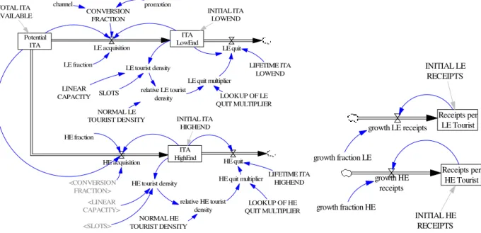
Figure 3: SD Base Line Model of ITA 2004-2030. ITA LowEnd Potential ITA _{LE acquisition} TOTAL ITA AVAILABLE LE quit LIFETIME ITA LOWEND LINEAR CAPACITY CONVERSION FRACTION relative LE tourist density NORMAL LE TOURIST DENSITY LE quit multiplier LOOKUP OF LE QUIT MULTIPLIER ITA HighEnd HE acquisition HE quit LIFETIME ITA HIGHEND HE quit multiplier LOOKUP OF HE QUIT MULTIPLIER INITIAL ITA LOWEND LE tourist density INITIAL ITA HIGHEND channel promotion <CONVERSION FRACTION> HE tourist density relative HE tourist density <LINEAR CAPACITY> NORMAL HE TOURIST DENSITY SLOTS <SLOTS> LE fraction HE fraction Receipts per HE Tourist growth HE receipts INITIAL HE RECEIPTS growth fraction HE Receipts per LE Tourist growth LE receipts INITIAL LE RECEIPTS growth fraction LE

The projected arrivals under the conditions of the Base Line model are represented in Figure 4.

Figure 4: Arrivals: Base Line Model

Arrivals : Base Line

15 M 11.25 M 7.5 M 3.75 M 0 2 2 2 2 2 2 2 2 2 2 2 2 2 2 2 2 2 2 2 ₂ 2 ₂ 2 ₂ 2 ₂ 2 1 1 1 1 1 1 1 ₁ 1 ₁ 1 ₁ 1 ₁ 1 1 ₁ 1 1 1 1 1 1 1 1 1 1 2004 2006 2008 2010 2012 2014 2016 2018 2020 2022 2024 2026 2028 2030 Time (Year)

ITA HighEnd : Current 1 1 1 1 1 1 1 1 1 1 1 1 1 1 1 1 1 1 1 1 1 1 tourist ITA LowEnd : Current 2 2 2 2 2 2 2 2 2 2 2 2 2 2 2 2 2 2 2 2 2 2 2 tourist

LE arrivals start at 9.9 million, and grow to their peak by the end of 2005, with 11.7 million arrivals. Thereafter, arrivals decline at a steep rate, reaching a low 1 million

in 2030. Meanwhile, the HE ITA curve shows lower amplitude, moving from an initial 1.7 million, to its peak of 3.3 million in 2008, and to a final 470,000 in 2030.

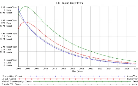
As suggested by Figure 5, the level of LE ITA is negatively impacted by a declining potential tourist population. The growth of the world market (Total ITA Available) cannot sustain the growth of Potential ITA (a share of 10%), out of which 15% are drained each year (LE acquisition) with a prospective 2-year lifetime only. The two curves are very similar in behaviour.

Figure 5: Flows affecting the level of LE ITA.

LE : In and Out Flows

8 M tourist/Year 1 Dmnl 80 M tourist 6 M tourist/Year 0.75 Dmnl 60 M tourist 4 M tourist/Year 0.5 Dmnl 40 M tourist 2 M tourist/Year 0.25 Dmnl 20 M tourist 0 tourist/Year 0 Dmnl 0 tourist 4 4 4 4 4 4 4 4 4 4 4 4 4 ₄ 4 ₄ 4 ₄ 3 3 3 3 3 3 3 3 3 3 3 3 3 3 3 3 3 3 ₃ 2 2 2 2 2 2 2 2 2 2 2 2 2 2 ₂ 2 ₂ 2 2 1 1 1 1 1 1 1 1 1 1 1 1 1 ₁ 1 ₁ 1 1 ₁ 2004 2006 2008 2010 2012 2014 2016 2018 2020 2022 2024 2026 2028 2030 Time (Year)

LE acquisition : Current 1 1 1 1 1 1 1 1 1 1 1 1 1 1 1 1 tourist/Year LE quit : Current 2 2 2 2 2 2 2 2 2 2 2 2 2 2 2 2 2 tourist/Year relative LE tourist density : Current 3 3 3 3 3 3 3 3 3 3 3 3 3 3 3 Dmnl Potential ITA : Current 4 4 4 4 4 4 4 4 4 4 4 4 4 4 4 4 4 tourist

As regards the outflow, the Quit rate coincides with the behaviour of the Relative LE Density, suggesting that it is never negatively impacted by the Quit Multiplier. Indeed, the Relative LE Tourist Density never goes above 1, and therefore never causes the multiplier to accelerate the LE Quit rate.

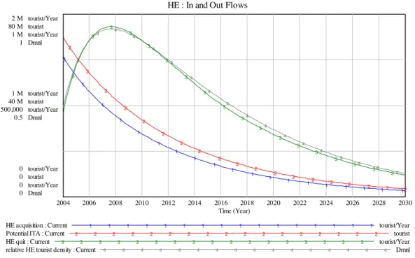
Contrary to expectations, density does not appear to play a negative feedback role. The lifetime is the key factor impacting the outflow. The validity of these insights will be tested by performing a sensitivity analysis further down. The same findings apply to HE ITA (see Fig. 6). The Quit Multiplier is always under 1, the relative tourist density being under 1 for the duration of the simulation.

Figure 6: Flows affecting the level of HE ITA.

HE : In and Out Flows

2 M tourist/Year 80 M tourist 1 M tourist/Year 1 Dmnl 1 M tourist/Year 40 M tourist 500,000 tourist/Year 0.5 Dmnl 0 tourist/Year 0 tourist 0 tourist/Year 0 Dmnl 4 4 4 ₄ 4 4 4 4 4 4 4 4 4 4 4 4 4 4 3 3 3 3 3 3 3 3 3 3 3 3 3 3 3 3 3 3 2 2 2 2 2 2 2 2 2 2 2 2 2 ₂ 2 2 ₂ 2 2 1 1 1 1 1 1 1 1 1 1 1 1 ₁ 1 ₁ 1 _{1 1} 1 2004 2006 2008 2010 2012 2014 2016 2018 2020 2022 2024 2026 2028 2030 Time (Year)

HE acquisition : Current 1 1 1 1 1 1 1 1 1 1 1 1 1 1 1 1 tourist/Year Potential ITA : Current 2 2 2 2 2 2 2 2 2 2 2 2 2 2 2 2 2 tourist HE quit : Current 3 3 3 3 3 3 3 3 3 3 3 3 3 3 3 3 3 tourist/Year relative HE tourist density : Current 4 4 4 4 4 4 4 4 4 4 4 4 4 4 4 4 Dmnl

The receipts (ITR) generated by both categories of tourists, as represented in Figure 7, are influenced not only by the volume, but also by the rate of receipts per tourist (the HE rate being twice the LE rate at the initial period), on one hand, and by the average rate growth on the other hand. The latter, as indicated in the assumptions, remains constant (at 3.19%) for LE tourists, but climbs from 3.19% to 5.25% for HE tourists.

The combination of these factors explains that, in spite of their much lower volume, HE ITA contribute more than LE ITA in absolute terms from 2023 onwards.

Figure 7: Projected Receipts – Base Line model 2004-2030.

Projected Tourist Receipts : Base Line

10 B 7.5 B 5 B 2.5 B 0 3 3 3 3 3 3 3 3 3 3 3 3 3 3 ₃ 3 ₃ 3 ₃ 3 ₃ 3 ₃ 3 ₃ 3 3 2 2 2 2 2 2 2 2 ₂ 2 ₂ 2 ₂ 2 ₂ 2 ₂ 2 ₂ 2 2 ₂ 2 ₂ 2 2 2 2 1 1 1 1 1 1 1 1 1 1 1 1 1 1 1 1 1 1 1 1 1 1 1 1 1 1 1 ₁ 2004 2006 2008 2010 2012 2014 2016 2018 2020 2022 2024 2026 2028 2030 Time (Year)

Total Receipts : Current 1 1 1 1 1 1 1 1 1 1 1 1 1 1 1 1 1 1 1 1 1 tourist*euro Cumul HE Receipts : Current 2 2 2 2 2 2 2 2 2 2 2 2 2 2 2 2 2 2 2 2 tourist*euro Cumul LE Receipts : Current 3 3 3 3 3 3 3 3 3 3 3 3 3 3 3 3 3 3 3 3 3 tourist*euro

7. Inferences from running the Base Line model

Briefly stated, I draw the following three (inferences are identified by the prefix in).

i1. The tourism business in Portugal may have reached or be about to reach its maturity

stage. This insight is supported by WTO data on Portugal’s ITA (decline of 3.2% from 2000 to 2003, source: WTO 2003, 2004) and by national data on Algarve (after a peak of 12.2 million foreigner stays in 2000, there were only 9.9 million in 2004, about the same as in 1992, source: DSET - DRAE 2005). What comes next? The decline stage should be expected. Typical policies to mitigate the adverse consequences are: actions aimed at extending the PLC (renovating the product or its marketing), “milking” the eroding market share (by changing pricing), or a combination of both. Which one should be recommended?

i2. The model suggests that a segmentation and targeting policy could be advantageously

developed and implemented. The goal is to capitalise on the better performing HE tourists (in terms of receipts), and discontinue the emphasis placed on volume LE

capacity)? Upgrading the marketing programmes to improve the yield? Launching relationship marketing programmes to strengthen customer loyalty, lengthen the tourist’s lifetime and enhance the tourist lifetime value?

8. The HE Focus Model

With a view to try and respond to these issues, the second HE Focus model focuses on high end tourist elite. It has a structure similar to the Base Line one, with only two changed parameters:

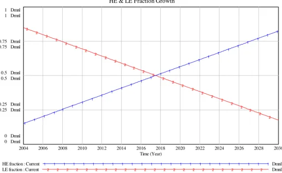
a. In the Base Line model, the initial split between LE and HE arrivals is 85% and 15% respectively, and it remains constant [assumption 4]. In the HE Focus Model, I assume that, by carefully targeting the high end tourists, the proportions will gradually turn upside down. The HE fraction of the market share will grow from 15% at the beginning of 2004 to 85% by the end of 2030, while the LE share will decay to 15%, as shown in Figure 8.

Figure 8: Mix of LE and HE tourists in the HE Focus Model.

HE & LE Fraction Growth

1 Dmnl 1 Dmnl 0.75 Dmnl 0.75 Dmnl 0.5 Dmnl 0.5 Dmnl 0.25 Dmnl 0.25 Dmnl 0 Dmnl 0 Dmnl 2 2 2 2 2 2 2 2 2 2 2 2 2 2 2 2 2 2 2 2 2 2 2 2 2 2 1 1 1 1 1 1 1 1 1 1 1 1 1 1 1 1 1 1 1 1 1 1 1 1 1 1 1 2004 2006 2008 2010 2012 2014 2016 2018 2020 2022 2024 2026 2028 2030 Time (Year) HE fraction : Current 1 1 1 1 1 1 1 1 1 1 1 1 1 1 1 1 1 1 1 1 1 1 1 1 Dmnl LE fraction : Current 2 2 2 2 2 2 2 2 2 2 2 2 2 2 2 2 2 2 2 2 2 2 2 Dmnl

b. I further assume that the yield of channel and promotional efforts will be slightly lower, given the new and more exclusive audiences. Instead of 10% for channels [assumption 3], the new value is 5% only.

The resulting projected arrivals exhibit quite a different profile, as shown in Figure 9. The initial growth of LE arrivals almost vanishes. Around 2015, HE arrivals catch up with LE arrivals, and remain higher all the way through 2030.

Figure 9: Arrivals: HE Focus Model.

Arrivals : HE Focus 12 M 9 M 6 M 3 M 0 2 2 2 2 2 2 2 2 2 2 2 2 2 2 2 2 2 2 2 2 2 ₂ 2 ₂ 2 ₂ 2 2 1 1 1 1 1 1 1 1 1 1 1 1 1 1 1 ₁ 1 ₁ 1 ₁ 1 1 ₁ 1 ₁ 1 ₁ 1 2004 2006 2008 2010 2012 2014 2016 2018 2020 2022 2024 2026 2028 2030 Time (Year)

ITA HighEnd : Current 1 1 1 1 1 1 1 1 1 1 1 1 1 1 1 1 1 1 1 1 1 1 tourist ITA LowEnd : Current 2 2 2 2 2 2 2 2 2 2 2 2 2 2 2 2 2 2 2 2 2 2 2 tourist

The impact on total ITA is presented in Figure 10, which shows the Total ITA under the Base Line and the HE Focus scenarios. The Base Line ITA behaviour may deceive until 2013, but as from 2014, the HE Focus policy performs obviously and considerably better than the Base Line, in spite of the lower yield of marketing. Indeed, the total area under the HE Focus ITA is slightly larger (102%) than the corresponding Base Line ITA, providing a testimony of the inferiority of the latter policy. An additional benefit is the far smoother evolution of ITA under the HE Focus scenario.

Figure 10: Total ITA – Base Line and HE Focus compared. ITA: Base Line (bl) and HE Focus (he) compared

0 2,000,000 4,000,000 6,000,000 8,000,000 10,000,000 12,000,000 14,000,000 16,000,000 200420052006200720082009201020112012201320142015201620172018201920202021202220232024202520262027202820292030 IT A bl_Total ITA he_Total ITA

Receipts also present another face altogether, much more welcoming. Figure 11 shows the curves of the projected receipts. Total receipts grow from an initial Euro 6.1 billion (WTO 2003, 2004) by the end of 2003, to reach 7.7 billion in late 2010, and smoothly decrease to 6.3 billion through 2030. This clearly outperforms the Base Line model, as illustrated in Figure 12.

Figure 11: Projected Receipts – HE Focus model 2004-2030.

Projected Tourist Receipts : HE Focus

8 B 6 B 4 B 2 B 0 3 3 3 3 3 3 3 3 3 3 3 3 3 3 ₃ 3 ₃ 3 ₃ 3 3 ₃ 3 ₃ 3 ₃ 3 3 2 2 ₂ 2 2 2 2 2 2 2 2 2 2 2 2 2 ₂ 2 2 ₂ 2 ₂ 2 ₂ 2 2 ₂ 2 1 1 1 1 1 1 1 1 1 1 1 1 1 1 1 1 1 1 1 1 1 1 1 1 1 1 1 1 2004 2006 2008 2010 2012 2014 2016 2018 2020 2022 2024 2026 2028 2030 Time (Year)

Cumul HE Receipts : Current 1 1 1 1 1 1 1 1 1 1 1 1 1 1 1 1 1 1 1 1 tourist*euro Cumul LE Receipts : Current 2 2 2 2 2 2 2 2 2 2 2 2 2 2 2 2 2 2 2 2 tourist*euro Total Receipts : Current 3 3 3 3 3 3 3 3 3 3 3 3 3 3 3 3 3 3 3 3 3 3 tourist*euro

The HE Focus approach may not appeal to short-termists, eager to make a fast return on investment. Indeed, as shown in Figure 12, the receipts generated by the Base Line policy remain superior to what the HE Focus can produce until 2011. This is a pleasant 7 year bonanza.

Afterwards though, HE Focus proves vastly superior. The cumulative receipts through 2030 show a clear 30% advantage for the HE Focus policy. Furthermore, not only the inflection point between the mature and the decline stages occurs much later, in fact 4 years later, but also the amplitude of the curve is significantly lower, allowing for a much smoother ride throughout the entire period. Not surprisingly the key contributors to this performance are the HE receipts, as shown in the chart (see Figure 11).

Figure 12: Total ITR – Base Line and HE Focus compared. ITR : Base Line (bl) and HE Focus (he) Compared

0 1,000 2,000 3,000 4,000 5,000 6,000 7,000 8,000 9,000 10,000 200420052006200720082009201020112012201320142015201620172018201920202021202220232024202520262027202820292030 E u ro ( m il li o n ) he Total ITR bl Total ITR

As a reality check of the HE Focus approach, Figure 13 illustrates the comparative development of arrivals and receipts for Portugal and Switzerland, 1990-2002 (WTO 2003). In spite of a dramatic fall of ITA (-25%) compared with Portugal’s growth of 45%, Switzerland succeeded in maintaining an enviable level of ITR (Euro 8 billion in 2002), 29% higher than Portugal’s (6.2 billion). As dramatic for individual tourism entrepreneurs as this situation may be, the Swiss case gives evidence that a downfall in ITA does not

Figure 13: ITA and ITR evolution for Switzerland and Portugal, 1990-2002. 0 1,000 2,000 3,000 4,000 5,000 6,000 7,000 8,000 9,000 1990 1995 2000 2001 2002* IT R ( E u ro m il li o n ) 0 2,000 4,000 6,000 8,000 10,000 12,000 14,000 IT A ( 1 0 0 0 ) ITR Switzerland ITR Portugal ITA Portugal ITA Switzerland

It is therefore highly likely that a HighEnd focussed policy can both extend the PLC, and better remunerate the tourism investment. It requires obviously a sharper segmentation of the market and a clear targeting on the high end segment. This responds to a large extent to the queries raised in inferences i1 and i2 from the Base Line model

above.

9. Performance Drivers

As regards the actions that promise a bigger bang for the buck (issue raised in inference i3), the sensitive analysis performed for both models offers some compelling results.

While building the model, I intuitively considered that a major driver could be the tourist’s reaction to the relative tourist density. The unmovable limit set by nature itself – the linear capacity – appeared to be a true stopper to tourist arrivals growth. In fact, as shown above, relative density never accelerated the quit fraction.

It would be therefore a sensible thing to do to change some variables, and explore the reaction of the system. For this purpose, I started by changing, first up to 1.5 and then down to 0.5, the parameters of the following variables, one at a time:

• Normal Density (assuming that, by some smart architectural design and resort planning, squeezing more people into a linear meter is a viable proposition) [assumption 6].

• Conversion Factor (assuming that savvier marketers could significantly improve yields of marketing programmes) [assumption 3].

• Lifetimes (assuming that effective customer relationship programmes could improve loyalty and client lifetime) [assumption 7].

Some outputs of the sensitivity analysis are shown in Figure 14 (see full set in Attachment 1). It results unequivocally that the key driver is the Lifetime. Both models, and both variations by plus or minus 50%, indicate that given the structure of the system, ITA and ITR react foremost to the variation of the lifetimes.

Figure 14.a: impact of 150% variation of 3 parameters on ITR (Base Line Model).

Cumul LE Receipts 6 B 4.5 B 3 B 1.5 B 0 4 4 4 4 4 4 4 4 4 4 ₄ 3 3 3 3 3 3 3 3 3 3 3 2 2 2 2 2 2 2 2 2 2 ₂ 1 1 1 1 1 1 1 1 1 ₁ 1 2004 2008 2012 2016 2020 2024 2028 Time (Year)

Cumul LE Receipts : dens ity 150% 1 1 1 1 1 1 tourist*euro

Cumul LE Receipts : conversion 150% 2 2 2 2 2 2 tourist*euro

Cumul LE Receipts : lifetime 150% 3 3 3 3 3 3 tourist*euro

Cumul LE Receipts : current 4 4 4 4 4 4 4 tourist*euro

Cumul HE Receipts 6 B 4.5 B 3 B 1.5 B 0 4 4 4 4 4 4 4 ₄ 4 ₄ 4 3 3 ₃ 3 3 3 3 3 3 3 ₃ 2 2 2 2 ₂ 2 2 2 2 2 ₂ 1 1 1 1 1 1 1 1 1 1 ₁ 2004 2008 2012 2016 2020 2024 2028 Time (Year)

Cumul HE Receipts : density 150% 1 1 1 1 1 1 touris t*euro

Cumul HE Receipts : lifetime 150% 2 2 2 2 2 2 touris t*euro

Cumul HE Receipts : conversion 150% 3 3 3 3 3 3 touris t*euro

Cumul HE Receipts : current 4 4 4 4 4 4 4 touris t*euro

Figure 14.b: impact of 150% variation of 3 parameters on ITR (HE Focus Model).

Cumul LE Receipts 6 B 4.5 B 3 B 1.5 B 4 4 4 4 4 4 4 4 4 4 3 3 3 3 3 3 3 3 3 3 3 2 2 2 2 2 2 2 2 2 1 1 1 1 1 1 1 1 1 1 1 Cumul HE Receipts 10 B 7.5 B 5 B 2.5 B 4 4 4 4 4 4 4 4 4 4 4 3 3 3 3 3 3 3 3 3 3 3 2 2 2 2 2 2 2 ₂ 2 ₂ 2 1 1 1 1 1 1 1 1 1 1 1

Of course, changes in other variables also impact results. The conversion factors cause ITA and ITR to exhibit a somewhat counterintuitive behaviour. However, in absolute terms, the crucial business variable is definitely the lifetime. When it is made to vary upwards, it pushes significantly up the ITR; when it moves downwards, it pulls the ITR down much more than a similar relative change of the other two variables.

10. Inferences from running the HE Focus model and performing the sensitivity analysis

i4. Under HE Focus model conditions, inference i1 according to which Portugal’s inbound

tourism is maturing is confirmed. And yet PLC curves have a quite different profile. As regards ITA, the HE Focus provides a much softer landing than the Base Line. As regards receipts, the benefits of HE Focus are head and shoulders superior. While the Base Line Model reaches the inflection point already in 2007, HE Focus only gets there in 2011. On the other hand, while the Base Line shows that tourism is already in the antechamber of the decline stage (starting in 2015, if we generously take decline to mean, not the deceleration of the growth rate, but that receipts get below the initial ITR absolute value), with the HE Focus policy the same situation occurs after 2030 only. This suggests that HE Focus is an appropriate marketing strategy to overcome the shortcomings of the present tourism business situation, and answers the core issue raised in inference i2 by pointing towards the extension of the PLC by means of

refocusing on more attractive segments.

i5. The HE Focus model supports and demonstrates inference i2. Segmentation and

targeting high end segments are far more rewarding strategies than chasing volume. i6. The sensitivity analysis suggests that the last option indicated in inference i3, i.e. the

emphasis on effective customer relationship programmes, with a view to lengthen lifetimes, is the prima facie best policy.

11. Conclusion

Strategy development for the tourism business, as for any other business, requires a basic understanding of the probable future evolution of sales and revenues. The PLC concept is the specific tool for this purpose.

Although PLC rests upon forecasting, its goal is not to predict, nor even to prescribe, but to provide an “if this – then that” workbench, where to perform what-if analyses and run tests on alternative policies and structures.

The statistical S-curve method, used in other industries, did not perform adequately in this tourism analysis. For this reason, I opted for a causal method, more specifically a

system dynamics model to represent the ITA and ITR systems under two different scenarios, Base Line and HE Focus.

Through simulation and sensitivity analysis I inferred policy recommendations for inbound international tourism that can be summarised in three statements:

1. Doing more of the same will likely lead to dramatic diminishing returns quite soon.

2. Segmenting the market, targeting the more exclusive tourists, and shifting the emphasis from the now predominantly low grade, to the high grade product offering are likely to generate the number of arrivals and the level of receipts required to sustain the business in the decades to come.

3. The lifecycle and the lifetime value of the tourist are likely the variables on which strategic decisions should be made with first priority.

This being said, I wish to close with three methodological remarks. The timings indicated in the model are purely indicative. They assume that there is no delay between decision making and actual decision implementation, and that other variables do not interact with the model; both assumptions are obviously not true. Of course, all models are wrong. And yet, most people use mental models to solve pressing problems. Often, the critical assumptions in any model, mental or formal, remain - alas -implicit. The modellers themselves are unaware of them and are caught by surprise by the unintended consequences of their decisions. Models fail because they do not fit the purpose, do not include important feedbacks or keep key variables implicit. The best policy to mitigate the risk is to make them fully replicable and available for review (Sterman 2002). This has been done here.

The frame of reference for this analysis is marketing, not economics. By marketing, one should understand, not the hegemonic promotion and communication issues that tend to fill the space in the official consideration of the subject matter, but the “behavioural science that seeks to explain exchange relationships” (Hunt 1983) dealing with (1) buyers and (2) sellers consummating exchanges, within the (3) institutional framework directed at consummating or facilitating exchanges, and (4) the consequences for society of these behaviours and the institutional framework. By considering the issue to be fundamentally a managerial and not an economic one, I suggest that the problem, if there is a problem, can be fixed by management praxis, while avoiding the trap of the stale debate of “market forces” against “state interventionism”.

Last comment, this contribution should be considered as work in progress, in fact as the first step in doing the job of developing and analysing alternative policies. A much

References

Armstrong, J. Scott & R.J. Brodie (1999), Forecasting for Marketing, in Graham J. Hooley and Michael K. Hussey (Eds.), Quantitative Methods in Marketing, Second Edition. London: International Thompson Business Press, pp. 92-119.

Arthur D. Little Inc. (1974), A System for Managing Diversity, Cambridge.

Barreca, S. (1999), Assessing Functional Obsolescence in a Rapidly Changing Marketplace, Birmingham AL, BCRI.

Bass, F. M. (1969), A New Product Growth for Model Consumer Durables, Management Science, 15, 5, 215-227.

Boyd, H. and O. Walker (2000), Marketing, London, FT Knowledge.

CCRA (Comissão de Coordenação da Região do Algarve) (1990), PROT Algarve – Opções para os Algarvios, Cenários.

Day, G. S. (1975), A Strategic Perspective on Product Planning, Journal of Contemporary Business, 4, pp 1-34.

Forrester, J. W. (1994), System Dynamics, Systems Thinking, and Soft OR, System Dynamics Review, vol.10, No. 2.

Hunt, S. D. (1983), General Theories and the Fundamental Explananda of Marketing, Journal of Marketing, 47 (Fall).

INE (Instituto Nacional de Estatísticas) (2005), Contas Nacionais Anuais Preliminares, Lisboa.

Kotler, P & G. Armstrong (1993), Marketing An Introduction, Third Edition, Englewood Cliffs, Prentice-Hall.

Levitt, T. (1965), Exploit the Product Life Cycle, Harvard Business Review, November/December 1965.

Mahajan, Vijay, E. Muller, and F. Bass (1993), New Product Diffusion Models, in J. Eliashberg and G. L. Lilien (Eds.), Handbooks in Operations Research and Management Science (Vol. Marketing), Amsterdam, Elsevier Science Publishers B.V., pp. 349-408. Modis, T. (2003), Complexity and Change, in The Futurist, May-June 2003, pp. 28-32. Modis, T. (1992) Predictions, New York, Simon and Schuster.

Oliva, R., J. Sterman and M. Giese (2002), Limits to Growth in the New Economy: Exploring

the ‘Get Big Fast’ Strategy in e-commerce, available at

http://www.people.hbs.edu/roliva/research/.

Porter, M. E. (1985), Competitive Advantage - Creating and Sustaining Superior Performance, New York, The Free Press.

Rogers, E. (1995), Diffusion of Innovation, 4th edition, New York, Free Press.

Sapir, J. (2003), Les trous noirs de la science économique – Essai sur l’impossibilité de penser le temps et l’argent, Paris, Seuil.

Simon, H. A. (1976), From Substantive to Procedural Rationality, in S. J. Latsis (ed.), Methods and Appraisals in Economics, Cambridge, Cambridge University Press,.

Simon, H. A. (1990), Prediction and Prescription in Systems Modeling, Operations Research, Vol. 38, No. 1, pp. 7-14.

Sterman, J. D. (1991), A Skeptic’s Guide to Computer Models, in G.O. Barney et al (eds.) Managing a Nation: The Microcomputer Software Catalog, Boulder CO, Westview Press, pp. 209-229.

Sterman, J. D. (2000), Business Dynamics: Systems Thinking and Modeling for a Complex World, New York, Irwin/McGraw-Hill.

Sterman, J.D. (2002), All Models Are Wrong: Reflections on Becoming a Systems Scientist, Systems Dynamics Review Vol. 18, No. 4, pp. 501-531.

Swan, J. E. and D. R. Rink (1980), Effective Use of Industrial Product Life Cycle Trends, in Marketing in the 80s, New York: American Marketing Association, pp. 198-9.

WTO (World Tourism Organization) (1995), Concepts, Definitions, and Classifications for Tourism Statistics. Technical Manual No. 1, Madrid.

WTO (World Tourism Organization) (2001), Tourism 2020 Vision, Madrid.

WTO (World Tourism Organization) (2004), Tourism Highlights Edition 2004, Madrid. WTO (World Tourism Organization) (2003), Tourism Market Trends, Madrid.

Appendix Tourism Model simulations

Base Line : ITA Base Line : Receipts

Arrivals : Base Line

20 M 15 M 10 M 5 M 0 2 2 2 2 2 2 2 2 ₂ 2 ₂ 2 ₂ 2 2 1 1 1 1 1 ₁ 1 1 1 1 1 1 1 1 1 2004 2008 2012 2016 2020 2024 2028 Time (Year)

ITA HighEnd : Current 1 1 1 1 1 1 1 1 1 1 tourist ITA LowEnd : Current 2 2 2 2 2 2 2 2 2 2 tourist

Projected Tourist Receipts : Base Line

15 B 11.25 B 7.5 B 3.75 B 0 3 3 ₃ 3 ₃ 3 ₃ 3 3 ₃ 3 3 _{3 3} 2 2 2 2 2 2 _{2 2} 2 2 2 2 2 2 1 1 1 ₁ 1 1 1 1 ₁ 1 ₁ 1 ₁ 1 ₁ 2004 2008 2012 2016 2020 2024 2028 Time (Year)

Total Receipts : baseline 1 1 1 1 1 1 1 1 1 tourist*euro Cumul HE Receipts : baseline 2 2 2 2 2 2 2 tourist*euro Cumul LE Receipts : baseline 3 3 3 3 3 3 3 3 tourist*euro

Base Line : ITA (lifetimes = 150%) Base Line : Receipts (lifetimes = 150%)

Arrivals : Base Line

20 M 15 M 10 M 5 M 0 2 2 2 2 2 2 2 2 2 2 ₂ 2 ₂ 2 ₂ 1 1 1 1 1 1 1 ₁ 1 1 1 1 1 1 1 2004 2008 2012 2016 2020 2024 2028 Time (Year)

ITA HighEnd : lifetime 150pc 1 1 1 1 1 1 1 1 1 tourist ITA LowEnd : lifetime 150pc 2 2 2 2 2 2 2 2 tourist

Projected Tourist Receipts : Base Line

15 B 11.25 B 7.5 B 3.75 B 0 3 3 3 ₃ 3 3 ₃ 3 ₃ 3 3 ₃ 3 3 2 2 2 2 2 2 _{2 2} 2 2 2 2 2 2 1 1 1 1 1 1 1 1 1 1 1 ₁ 1 ₁ 1 2004 2008 2012 2016 2020 2024 2028 Time (Year)

Total Receipts : lifetime 150pc 1 1 1 1 1 1 1 1tourist*euro Cumul HE Receipts : lifetime 150pc 2 2 2 2 2 2 tourist*euro Cumul LE Receipts : lifetime 150pc 3 3 3 3 3 3 3 tourist*euro

Base Line : ITA (conversion = 150%) Base Line: Receipts (conversion = 150%)

Arrivals : Base Line

20 M 15 M 10 M 5 M 0 2 2 2 2 2 2 2 2 2 2 2 ₂ 2 2 2 1 1 1 1 ₁ 1 ₁ 1 ₁ 1 1 1 1 1 1 2004 2008 2012 2016 2020 2024 2028 Time (Year)

ITA HighEnd : conversion 150pc 1 1 1 1 1 1 1 1 tourist ITA LowEnd : conversion 150pc 2 2 2 2 2 2 2 2 tourist

Projected Tourist Receipts : Base Line

15 B 11.25 B 7.5 B 3.75 B 0 3 3 3 3 3 3 3 ₃ 3 ₃ 3 3 3 3 2 2 2 2 ₂ 2 ₂ 2 ₂ 2 ₂ 2 2 2 1 1 1 1 1 1 1 1 1 1 1 ₁ 1 ₁ 1 2004 2008 2012 2016 2020 2024 2028 Time (Year)

Total Receipts : conversion 150pc 1 1 1 1 1 1 1 tourist*euro Cumul HE Receipts : conversion 150pc 2 2 2 2 2 2 tourist*euro Cumul LE Receipts : conversion 150pc 3 3 3 3 3 3 tourist*euro

Base Line : ITA (norm. density = 150%) Base Line: Receipts (norm. density = 150%)

Arrivals : Base Line

20 M 15 M 10 M 5 M 0 2 2 2 2 2 2 2 2 2 2 2 ₂ 2 ₂ 2 1 1 1 1 1 1 1 ₁ 1 ₁ 1 1 1 1 1 2004 2008 2012 2016 2020 2024 2028 Time (Year)

ITA HighEnd : norm.density 150pc 1 1 1 1 1 1 1 1 tourist ITA LowEnd : norm.density 150pc 2 2 2 2 2 2 2 tourist

Projected Tourist Receipts : Base Line

15 B 11.25 B 7.5 B 3.75 B 0 3 3 3 3 3 ₃ 3 ₃ 3 ₃ 3 ₃ 3 3 2 2 2 2 2 2 2 2 2 ₂ 2 2 2 2 1 1 1 1 ₁ 1 1 1 1 1 1 1 1 ₁ 1 2004 2008 2012 2016 2020 2024 2028 Time (Year)

Total Receipts : norm.density 150pc 1 1 1 1 1 1 1 tourist*euro Cumul HE Receipts : norm.density 150pc 2 2 2 2 2 tourist*euro Cumul LE Receipts : norm.density 150pc 3 3 3 3 3 3 tourist*euro

Base Line Model simulations: sensitivity analysis

Base Line: ITA (LowEnd): var. 150% Base Line: Receipts (LowEnd): var. 150%

ITA LowEnd 20 M 15 M 10 M 5 M 4 4 4 4 4 3 3 3 3 3 2 2 2 2 2 2 2 1 1 1 1 1 1 Cumul LE Receipts 8 B 6 B 4 B 2 B 4 4 4 4 4 4 4 4 3 3 3 3 3 3 3 2 2 2 2 2 2 2 2 2 2 2 1 1 1 1 1 1 1 1 1

Base Line: ITA (HighEnd): var. 150% Base Line: Receipts (HighEnd) : var. 150% ITA HighEnd 6 M 4.5 M 3 M 1.5 M 0 4 4 4 4 4 4 4 4 4 ₄ 4 3 3 3 3 3 3 3 3 3 ₃ 3 2 2 2 2 2 2 2 2 2 2 2 1 1 1 1 1 1 1 1 1 ₁ 1 2004 2008 2012 2016 2020 2024 2028 Time (Year)

ITA HighEnd : density 150% 1 1 1 1 1 1 1 tourist

ITA HighEnd : lifetime 150% 2 2 2 2 2 2 2 2 tourist

ITA HighEnd : conversion 150% 3 3 3 3 3 3 3tourist

ITA HighEnd : current 4 4 4 4 4 4 4 4 tourist

Cumul HE Receipts 6 B 4.5 B 3 B 1.5 B 0 4 4 4 4 4 4 4 4 4 ₄ 4 3 3 ₃ 3 3 3 3 3 3 3 ₃ 2 2 2 2 ₂ 2 2 2 2 2 2 1 1 1 ₁ 1 1 1 1 1 1 1 2004 2008 2012 2016 2020 2024 2028 Time (Year)

Cumul HE Receipts : density 150% 1 1 1 1 1 1 tourist*euro

Cumul HE Receipts : lifetime 150% 2 2 2 2 2 2 tourist*euro

Cumul HE Receipts : conversion 150% 3 3 3 3 3 3 tourist*euro

Cumul HE Receipts : current 4 4 4 4 4 4 4tourist*euro

Base Line: ITA (LowEnd): var. 50% Base Line: Receipts (LowEnd): var. 50%

ITA LowEnd 20 M 15 M 10 M 5 M 0 4 4 4 4 4 4 ₄ 4 _{4 4} 4 3 3 3 3 3 ₃ 3 ₃ 3 ₃ 3 2 2 2 2 ₂ 2 _{2 2} 2 2 2 1 1 1 1 1 1 1 ₁ 1 1 ₁ 2004 2008 2012 2016 2020 2024 2028 Time (Year)

ITA LowEnd : baseline_density 50% 1 1 1 1 1 1 tourist

ITA LowEnd : baseline_lifetime 50% 2 2 2 2 2 2 2 tourist

ITA LowEnd : baseline_conversion 50% 3 3 3 3 3 3tourist

ITA LowEnd : Current 4 4 4 4 4 4 4 4 tourist

Cumul LE Receipts 6 B 4.5 B 3 B 1.5 B 0 4 4 4 4 4 4 4 4 4 4 4 3 3 3 3 3 ₃ 3 ₃ 3 ₃ 3 2 2 2 2 2 2 2 2 ₂ 2 ₂ 1 1 1 1 1 1 1 1 1 1 1 2004 2008 2012 2016 2020 2024 2028 Time (Year)

Cumul LE Receipts : baseline_density 50% 1 1 1 1 1 tourist*euro

Cumul LE Receipts : baseline_lifetime 50% 2 2 2 2 2 tourist*euro

Cumul LE Receipts : baseline_conversion 50% 3 3 3 3 3 tourist*euro

Cumul LE Receipts : Current 4 4 4 4 4 4 4 tourist*euro

Base Line: ITA (HighEnd): var. 50% Base Line: Receipts (HighEnd) : var. 50%

ITA HighEnd 4 M 3 M 2 M 1 M 0 4 4 4 4 4 4 4 4 4 4 ₄ 3 3 3 ₃ 3 3 3 3 ₃ 3 ₃ 2 2 2 2 2 2 2 ₂ 2 _{2 2} 1 1 1 1 1 1 1 1 1 1 ₁ 1 2004 2008 2012 2016 2020 2024 2028 Time (Year)

ITA HighEnd : baseline_density 50% 1 1 1 1 1 1 tourist

ITA HighEnd : baseline_lifetime 50% 2 2 2 2 2 2 2 tourist

ITA HighEnd : baseline_conversion 50% 3 3 3 3 3 3tourist

ITA HighEnd : Current 4 4 4 4 4 4 4 4 tourist

Cumul HE Receipts 4 B 3 B 2 B 1 B 0 4 4 4 4 4 4 4 4 4 4 4 3 3 3 3 3 3 _{3 3} 3 _{3 3} 2 2 2 2 2 2 2 2 ₂ 2 2 1 1 1 ₁ 1 1 1 1 1 1 1 ₁ 2004 2008 2012 2016 2020 2024 2028 Time (Year)

Cumul HE Receipts : baseline_density 50% 1 1 1 1 1 tourist*euro

Cumul HE Receipts : baseline_lifetime 50% 2 2 2 2 2 tourist*euro

Cumul HE Receipts : baseline_conversion 50% 3 3 3 3 3 tourist*euro

HE Focus Model simulations

HE Focus: ITA HE Focus: Receipts

Arrivals : HE Focus 12 M 9 M 6 M 3 M 0 2 2 2 2 2 2 2 2 2 2 ₂ 2 ₂ 2 2 1 1 1 1 1 1 1 1 1 _{1 1} 1 _{1 1} 1 2004 2008 2012 2016 2020 2024 2028 Time (Year)

ITA HighEnd : Current 1 1 1 1 1 1 1 1 1 1 tourist ITA LowEnd : Current 2 2 2 2 2 2 2 2 2 2 tourist

Projected Tourist Receipts : HE Focus

15 B 11.25 B 7.5 B 3.75 B 0 3 3 3 3 3 3 3 3 3 3 3 3 3 3 2 2 ₂ 2 ₂ 2 _{2 2} 2 2 _{2 2} 2 2 1 1 1 1 1 1 1 1 1 1 1 1 1 1 1 2004 2008 2012 2016 2020 2024 2028 Time (Year)

Cumul HE Receipts : Current 1 1 1 1 1 1 1 1 tourist*euro Cumul LE Receipts : Current 2 2 2 2 2 2 2 tourist*euro Total Receipts : Current 3 3 3 3 3 3 3 3 3 tourist*euro

HE Focus : ITA (lifetimes = 150%) HE Focus : Receipts (lifetimes = 150%)

Arrivals : HE Focus 12 M 9 M 6 M 3 M 0 2 2 2 2 2 2 2 2 2 2 2 2 2 2 ₂ 1 1 1 1 1 1 1 1 1 ₁ 1 ₁ 1 ₁ 1 2004 2008 2012 2016 2020 2024 2028 Time (Year)

ITA HighEnd : lifetimes 150pc 1 1 1 1 1 1 1 1 1 tourist ITA LowEnd : lifetimes 150pc 2 2 2 2 2 2 2 2 tourist

Projected Tourist Receipts : HE Focus

15 B 11.25 B 7.5 B 3.75 B 0 3 3 3 3 3 3 3 3 3 3 3 3 3 3 2 2 2 2 ₂ 2 ₂ 2 ₂ 2 ₂ 2 2 ₂ 1 1 1 1 1 1 1 1 1 1 1 1 1 1 1 2004 2008 2012 2016 2020 2024 2028 Time (Year)

Cumul HE Receipts : lifetimes 150pc 1 1 1 1 1 1 1 tourist*euro Cumul LE Receipts : lifetimes 150pc 2 2 2 2 2 2 tourist*euro Total Receipts : lifetimes 150pc 3 3 3 3 3 3 3 tourist*euro

HE Focus : ITA (conversion = 150%) HE Focus : Receipts (conversion = 150%)

Arrivals : HE Focus 12 M 9 M 6 M 2 ₂ 2 2 2

Projected Tourist Receipts : HE Focus

15 B 11.25 B 7.5 B 3 3 3 ₃ 3 3 ₃ 3 3 ₃

HE Focus: ITA (norm. density = 150%) HE Focus:Receipts (norm. density = 150%) Arrivals : HE Focus 12 M 9 M 6 M 3 M 0 2 2 2 2 2 2 2 2 2 2 2 2 ₂ 2 2 1 1 1 1 1 1 1 1 1 ₁ 1 1 ₁ 1 ₁ 2004 2008 2012 2016 2020 2024 2028 Time (Year)

ITA HighEnd : density 150pc 1 1 1 1 1 1 1 1 1 tourist ITA LowEnd : density 150pc 2 2 2 2 2 2 2 2 tourist

Projected Tourist Receipts : HE Focus

15 B 11.25 B 7.5 B 3.75 B 0 3 3 3 3 3 3 3 3 3 3 3 3 3 3 2 2 ₂ 2 ₂ 2 ₂ 2 _{2 2} 2 2 2 2 1 1 1 1 1 1 1 1 1 1 1 1 1 1 1 2004 2008 2012 2016 2020 2024 2028 Time (Year)

Cumul HE Receipts : density 150pc 1 1 1 1 1 1 1 tourist*euro Cumul LE Receipts : density 150pc 2 2 2 2 2 2 tourist*euro Total Receipts : density 150pc 3 3 3 3 3 3 3 3 tourist*euro

HE Focus Model simulations: sensitivity analysis

HE Focus: ITA (LowEnd): var. 150% HE Focus: Receipts (LowEnd): var. 150%

ITA LowEnd 20 M 15 M 10 M 5 M 0 4 4 4 4 4 4 4 ₄ 4 4 4 3 ₃ 3 3 3 3 3 3 3 ₃ 3 2 2 2 2 2 2 2 ₂ 2 2 2 1 1 1 1 1 1 1 ₁ 1 ₁ 1 2004 2008 2012 2016 2020 2024 2028 Time (Year)

ITA LowEnd : density 150% 1 1 1 1 1 1 1 tourist

ITA LowEnd : conversion 150% 2 2 2 2 2 2 2 tourist

ITA LowEnd : lifetime 150% 3 3 3 3 3 3 3 3tourist

ITA LowEnd : current 4 4 4 4 4 4 4 4 tourist

Cumul LE Receipts 6 B 4.5 B 3 B 1.5 B 0 4 4 4 4 4 4 4 4 4 4 4 3 3 3 3 3 3 3 3 3 3 3 2 2 2 2 2 2 2 2 2 2 ₂ 1 1 1 1 1 1 1 1 1 1 1 2004 2008 2012 2016 2020 2024 2028 Time (Year)

Cumul LE Receipts : density 150% 1 1 1 1 1 1 tourist*euro

Cumul LE Receipts : conversion 150%2 2 2 2 2 2 tourist*euro

Cumul LE Receipts : lifetime 150% 3 3 3 3 3 3 tourist*euro

Cumul LE Receipts : current 4 4 4 4 4 4 4tourist*euro

HE Focus: ITA (HighEnd): var. 150% HE Focus: Receipts (HighEnd): var. 150%

ITA HighEnd 6 M 4.5 M 3 M 1.5 M 0 4 4 4 4 4 ₄ 4 4 4 4 4 3 3 3 3 3 3 3 3 3 3 3 2 2 2 2 2 2 2 2 2 2 2 1 1 1 1 1 1 1 1 1 1 1 2004 2008 2012 2016 2020 2024 2028 Time (Year)

ITA HighEnd : density 150% 1 1 1 1 1 1 1 tourist

ITA HighEnd : conversion 150% 2 2 2 2 2 2 2 tourist

ITA HighEnd : lifetime 150% 3 3 3 3 3 3 3 3tourist

ITA HighEnd : current 4 4 4 4 4 4 4 4 tourist

Cumul HE Receipts 10 B 7.5 B 5 B 2.5 B 0 4 4 4 4 4 4 4 4 4 4 4 3 3 3 3 3 3 3 3 3 3 3 2 2 2 2 2 2 2 ₂ 2 ₂ 2 1 1 1 1 1 1 1 1 1 1 1 2004 2008 2012 2016 2020 2024 2028 Time (Year)

Cumul HE Receipts : density 150% 1 1 1 1 1 1 tourist*euro

Cumul HE Receipts : conversion 150% 2 2 2 2 2 tourist*euro

Cumul HE Receipts : lifetime 150% 3 3 3 3 3 3 tourist*euro