Deformable registration, dose remapping and summation for head and neck adaptative radiotherapy applications

(1)

DEPARTAMENTO DE F´ISICA

Deformable Registration, Dose

Remapping and Summation for Head

and Neck Adaptive Radiotherapy

Applications

Ana M´

onica Ferreira de Almeida Louren¸

co

Disserta¸c˜ao

Mestrado Integrado em Engenharia Biom´edica e Biof´ısica Perfil em Sinais e Imagens M´edicas

(2)

(3)

DEPARTAMENTO DE F´ISICA

Deformable Registration, Dose

Remapping and Summation for Head

and Neck Adaptive Radiotherapy

Applications

Ana M´

onica Ferreira de Almeida Louren¸

co

Disserta¸c˜ao

Mestrado Integrado em Engenharia Biom´edica e Biof´ısica Perfil em Sinais e Imagens M´edicas

Orientador externo: Professor Doutor Gary Royle Orientador interno: Professor Doutor Eduardo Ducla Soares

(4)

(5)

Um tratamento de radioterapia tem como objectivo aplicar a dose máxima ao volume tumoral, provocando a sua morte celular, e preservar ao máximo os órgãos de risco (tecidos adjacentes saudáveis). Existem diferentes técnicas de entrega da radia¸cão, como por exemplo, a radioterapia conformal e a radioterapia de intensidade modulada. A radioterapia conformal permite o ajuste dos múltiplos feixes de radia¸cão à forma do alvo tumoral. Con-siderando múltiplos feixes à volta de um isocentro e que cada feixe tem uma fluência uniforme, então o volume da sua interseçcão será uma forma convexa sem qualquer concavidade. Contudo, os volumes tumorais podem apresentar formas côncavas. A radioterapia de intensidade modulada é uma técnica de radioterapia conformal que entrega a radia¸cão de uma forma mais precisa, reduzindo a dose emitida aos tecidos adjacentes saudáveis, e adequando as distribui¸cões de dose a alvos que tenham formas côncavas.

Na pr´atica cl´ınica de radioterapia de intensidade modulada, o tratamento ´

e planeado tendo como base imagens médicas do paciente, adquiridas antes do come¸co do mesmo, sendo o tratamento delineado e simulado numa única imagem de tomografia computorizada (TC de planeamento). Deste modo, ao longo do tratamento assume-se que a localiza¸cão, a geometria e o tamanho do volume tumoral e dos órgãos de risco são constantes. Contudo, durante um t´ıpico tratamento de radioterapia, que dura cerca de 5 a 7 semanas, podem ocorrer potenciais modifica¸cões anatómicas e de posicionamento do paciente. Estas varia¸cões podem ser ainda mais significativas para pacientes oncológicos de cabe¸ca e pesco¸co, uma vez que, a rápida redu¸cão do volume do tumor primário, a perda de peso e as altera¸cões na distribui¸cão de gordura e músculo são frequentes nestes pacientes, o que pode causar significativa discordância entre a distribui¸cão da dose planeada e aquela que está a ser efectivamente entregue, provocando toxicidade. Nestas situa¸cões, uma nova TC de planeamento é adquirida durante o tratamento e todo o processo de planeamento é repetido. Desta maneira, o replaneamento consiste num pro-cesso que consome tempo e recurso cl´ınicos.

(6)

sala de tratamento, como por exemplo, imagens de tomografia de feixe cónico (TCFC), para reavaliar sistematicamente a localiza¸cão e a forma do volume tumoral. Estas novas imagens podem ser usadas para o cálculo de distribui¸cões de dose diária e cumulativa que incorporem as varia¸cões anatómicas e de posicionamento no planeamento do tratamento. Deste modo, a radioterapia adaptativa depende da radioterapia guiada por imagem (IGRT), da verifica¸cão constante das distribui¸cões de dose e da adapta¸cão do plano inicial à anatomia corrente do paciente. Os algoritmos de registro de imagens possibilitam o uso de imagens de TCFC em radioterapia adaptativa, permitindo a adapta¸cão do plano inicial de tratamento à anatomia actual do paciente. A TC de planeamento (pTC) pode ser deformada de acordo com a TCFC, produzindo uma nova imagem (pTC deformada), que tem a qualidade de imagem da pTC mas que contém a informa¸cão estrutural da TCFC. Deste modo, aplicando as configura¸cões dos feixes do plano inicial `

a anatomia da nova imagem registrada, novos c´alculos de dose podem ser efectuados na imagem de pTC deformada.

O presente estudo teve como objectivo o desenvolvimento de um método para calcular a distribui¸cão da dose cumulativa recebida por pacientes oncológicos da cabe¸ca e pesco¸co ao longo dos seus tratamentos, através de avan¸cadas técnicas de registro de imagens (usando transformadas B-Spline) que incorporam as varia¸cões anatómicas e de posicionamento que possam ocorrer. Neste estudo, foram inclu´ıdos 5 pacientes com cancro da cabe¸ca e pesco¸co. Os pacientes foram tratados com radioterapia de intensidade modulada e, durante o tratamento, verificaram-se significativas varia¸cões anatómicas em todos os pacientes, o que resultou em 4 deles terem sido sujeitos a replaneamento. O processo de soma de dose utilizado consistiu no subsequente processo descrito. A imagem de pTC é registrada a uma série de imagens de TCFC adquiridas ao longo do tratamento. O output deste processo é uma série de transforma¸cões T que deformam a imagem de pTC de acordo com as altera¸cões anatómicas que ocorreram no paciente. Novos cálculos de dose são realizados em cada imagem de pTC deformada, usando o plano de tratamento inicial, e as distribui¸cões de dose são mapeadas de volta para o espa¸co da dose da pTC usando o inverso da transforma¸cão T−1. A aplica¸cão da transformada inversa permite mapear as novas distribui¸cões de dose, que incorporam as modifica¸cões anatómicas e de posicionamento que possam ter ocorrido, para o mesmo referencial (espa¸co da dose da

(7)

B-Spline T−1, não existe solu¸cão anal´ıtica para o seu cálculo.

Este estudo teve como principal objectivo estudar e avaliar o desempenho de três diferentes métodos que estimam T−1: (i) o método não-simétrico, (ii) o método simétrico (iii) e métodos de estima¸cão iterativos. O desem-penho de cada método é avaliado com base na (i) inspeçcão visual dos resultados do processo de registro de imagens e na (ii) computa¸cão de medidas de similaridade, que garantem a qualidade de correspondência entre as imagens, no (iii) cálculo do Jacobiano e no (iv) erro de consistência inversa que asseguram que as transforma¸cões (T e T−1) são fisicamente plaus´ıveis. Diferentes distribui¸cões de dose, obtidas através dos difer-entes métodos de computa¸cão da inversa, foram comparadas através da análise de diferen¸cas de dose e gamma análise, e histogramas dose-volume foram gerados para estudar os efeitos dosimétricos em estruturas de interesse. O método de estima¸cão iterativa foi o que apresentou os resultados mais robustos em termos de consistência entre a transformada T e a transformada T−1, com um erro médio de 0.009 mm. O método não simétrico apresentou um erro médio de 1.793 mm e o método simétrico um erro médio de 0.500 mm. Relativamente aos efeitos dosimétricos, os diferentes métodos de computa¸cão de T−1 mostraram performances semelhantes entre si. Para diferentes distribui¸cões de dose, as curvas dos histogramas dose-volume sobrepuseram-se consideravelmente e a diferen¸ca absoluta de dose máxima em órgãos de risco foi inferior a 1.1 Gy. Os valores aqui apresentados representam valores medianos sobre todos os pacientes considerados.

Os resultados mostraram que os métodos de computa¸cão da inversa de uma transformada B-Spline têm potencial para serem utilizados no cálculo da dose cumulativa e no cálculo da dose recebida pelo paciente em cada semana do tratamento.

A disserta¸cão encontra-se dividida em 5 grandes cap´ıtulos. O primeiro consiste numa introdu¸cão ao tema da disserta¸cão e no segundo são de-scritos os principais conceitos inerentes ao trabalho desenvolvido, como por exemplo, conceitos de radioterapia, planeamento e registro de imagens. São também descritos os diferentes algoritmos considerados e os métodos utilizados no seu processo de valida¸cão. O terceiro cap´ıtulo descreve os materiais e as metodologias utilizadas e o quarto os resultados obtidos. Discussão e conclusões encontram-se no quinto cap´ıtulo.

(8)

(9)

Purpose

The aim of this study was to assess and evaluate different methods of computing the inverse of a B-Spline transformation in order to calculate the cumulative doses received by head and neck (HN) cancer patients while accounting for variable anatomy.

Materials and Methods

Five patients with HN cancer were treated with IMRT and 4 of them were replanned midtreatment. Planning CT scan and CBCT image taken before replan were available. Planning CT images were registered to the CBCT scans and new dose calculations were performed in the deformed pCT images using the treatment IMRT plan. Dose distributions were mapped back to the pCT dose space using different methods of computing the inverse of a B-Spline transformation: (i) non-symmetric, (ii) symmetric and (iii) estimate the inverse methods. Their performance was evaluated based on visual inspection of registration results and computation of similarity measures, deformation field analysis and calculation of the inverse consistent error between the composition of forward and inverse transformations. Furthermore, dose comparisons were performed using dose difference (DD) and gamma analysis and dose volume histograms (DVH) were generated to study the dosimetric effects.

Results

Estimating the inverse methods gave the most robust results in terms of inverse-consistency between the composition of forward and inverse transformations with a median mean IC error of 0.009 mm. Regarding the dosimetric effects, results were found to be consistent between different inverse transforms. DVHs overlapped considerably and median values for maximum absolute dose differences in organs at risk were found to be less than 1.1 Gy.

(10)

B-Spline transformation, allowing the calculation of cumulative doses while accounting for anatomic variations.

Key-words: Adaptive Radiotherapy, Deformable Registration, Dose summation, B-Spline Transform, Inverse of a B-Spline transform

(11)

I would like to express my gratitude to everyone who made my stay in the University College London (UCL) so special and rewarding, there are no words to describe how happy and proud I am to have met them and to have had the opportunity to contact and work with them.

Firstly, I must thank to my supervisor Gary Royle, from the University College London (UCL) who gave me the opportunity to go abroad and this project. I also want to thank him for his clear guidance, generosity and encouragement and for always being available, I appreciate his vast knowledge and skill in many areas. A special thank to Jamie McClelland and Catarina Veiga who were so patient and glad to teach me everything I wanted to know even thought they are very busy with their work, they always found a time for me. Their dedication, expertise, understanding and patience added considerably to my project. I have the most respect for them and they are an inspiration to me as scientists and human beings.

I would also like to thank very much to Marcel Van Herk who provided me the estimate 1 inverse transform code which was crucial to the success of this project.

Also a big thank you to all the staff of the Radiotherapy Physics group from University College London Hospital who so well received me and provided me the data I needed for this project.

I am deeply thankful and I want to express a very special thanks to Professor Eduardo Ducla Soares for his guidance and encouragement during the time I have been his student in the Faculty of Sciences of the University of Lisbon. His unceasing support and motivation were crucial for my achievements in the last 5 years.

(12)

and for the great moments and happy times we spent together. I also would like to thank Paul, Marco, Joanna and Charlotte for being part of our running club, especially George and Tom which adventure spirit inspired me.

In addition, a very special thanks to my Stockwell’s family, Rui, Sara and Andreia for being the family I needed when I was miles away from home. And also to my London friends, Joanna and Ant´onio, for their friendship, love and wise advices.

There are no words to describe how grateful I am to my wonderful parents Maria and Júlio, my sisters Cátia and Júlia, my aunt Gotty and my cousin Rafa, and my friends Inês, Andrade, Maria, Mariana and Rita who always support me and were always by my side.

(13)

Resumo i

Abstract v

Acknowledgements vii

List of Tables xii

List of Figures xiii

List of Abbreviation xv

1 Introduction 1

2 Background 3

2.1 Radiotherapy . . . 3

2.1.1 Intensity modulated radiation therapy . . . 3

2.1.1.1 Volumetric modulated arc therapy . . . 4

2.1.2 Adaptive Radiotherapy . . . 4

2.1.3 Current practice of a Radiotherapy treatment at Uni-versity College London Hospital . . . 5

2.1.3.1 Volume delineation . . . 6

2.1.3.2 Computed tomography . . . 8

2.1.3.3 Cone beam computed tomography . . . 8

2.2 Medical image registration . . . 9

2.2.1 Transformation models . . . 9 2.2.1.1 Rigid transformations . . . 9 2.2.1.2 Non-rigid transformations . . . 10 2.2.1.3 B-Spline transformation . . . 11 2.2.1.3.1 B-Spline Curves . . . 11 2.2.1.4 B-Spline interpolation . . . 12

(14)

2.2.2 Inverse transformation models . . . 14

2.2.2.1 Asymmetric transformation . . . 15

2.2.2.2 Symmetric inverse consistent transformation . 15 2.2.2.3 Estimating the inverse of a B-Spline transfor-mation . . . 16

2.2.3 Validation process: quality criteria . . . 17

2.2.3.1 Image matching quality . . . 17

2.2.3.1.1 Visual assessment . . . 17

2.2.3.1.2 Similarity measures . . . 18

2.2.3.2 Deformation field analysis . . . 20

2.2.3.2.1 Jacobian . . . 20

2.2.3.2.2 Inverse consistent error . . . 20

2.2.4 Dose comparison . . . 21

2.2.4.1 Relative dose difference . . . 22

2.2.4.2 Distance-to-agreement . . . 22

2.2.4.3 Gamma evaluation . . . 22

2.2.4.4 Dose-volume histograms . . . 24

2.3 Previous work . . . 25

3 Materials and methods 27 3.1 Data sets . . . 27

3.1.1 DICOM . . . 27

3.2 Data Processing . . . 28

3.2.1 Image Registration - Performed in NifTK . . . 28

3.2.1.1 Forward asymmetric registration . . . 29

3.2.1.2 Inverse of the transformation . . . 30

3.2.1.2.1 Backward asymmetric registration . 30 3.2.1.2.2 Symmetric registration . . . 31

3.2.1.2.3 Estimate the inverse methods - Per-formed in Matlab/NifTK . . . 31

3.2.2 Dose Calculation - Performed in Eclipse . . . 32

3.2.3 Dose Summation - Performed in Matlab . . . 32

3.2.4 Deformed dose - Performed in NifTK . . . 34

3.3 Evaluation tools . . . 35

3.3.1 Visual assessment and similarity measures . . . 35

3.3.1.1 Forward transform . . . 36

3.3.1.2 Inverse transform . . . 36

3.3.1.3 Inverse consistence criterion . . . 36

3.3.1.4 Symmetric registration . . . 38

3.3.2 Deformation field analysis . . . 39

(15)

4 Results 40

4.1 Symmetric registration performance . . . 40

4.2 Evaluation of different inverse transform methods . . . 43

4.2.1 Similarity comparison . . . 43

4.2.2 Dosimetric comparison . . . 49

4.3 Cumulative dose calculation . . . 53

4.4 Comparison of deformed pCT dose and recalculated dose . . . 56

5 Discussion and conclusion 59 Bibliography 61 Appendix 72 A Matlab code 72 A.1 Dose summation process . . . 72

(16)

4.1 Symmetric registration performance. IC error results for Pa-tient X. . . 41 4.2 Symmetric registration performance. IC error results for

Pa-tient X, Y and Z. . . 43 4.3 Registration performance in the forward direction: NMI results. 44 4.4 Registration performance in the backward direction: NMI

re-sults. . . 45 4.5 Inverse consistency between transformations: normalized

cross correlation results shown in a table. . . 48 4.6 Inverse consistent error. . . 49 4.7 Dose comparison between different inverse transforms: dose

difference and gamma tests. . . 50 4.8 Dose comparison between different inverse transforms:

maxi-mum absolute dose differences in organs at risk . . . 50 4.9 Dose summation comparison between different inverse

trans-forms: dose difference and gamma tests . . . 53 4.10 Dose summation comparison between different inverse

trans-forms: maximum absolute dose differences in organs at risk . . 53 4.11 Dose comparison between recalculated dose in the deformed

pCT and deformed pCT dose: dose difference and gamma tests 57 4.12 Dose comparison between recalculated dose in the deformed

pCT and deformed pCT dose: maximum absolute dose differ-ences in organs at risk . . . 57

(17)

2.1 IMRT’s traversing plastic blocks . . . 4

2.2 Diagram to illustrate the main structures of interest in radio-therapy. . . 7

2.3 Example showing the difference between rigid and non-rigid registration. . . 10

2.4 Example of a displacement vector field. . . 11

2.5 B-Spline Basis Function. . . 12

2.6 B-Spline curves with different values of scaling factors. . . 12

2.7 2D example of a B-Spline control-point grid superimposed upon an aligned voxel grid. . . 13

2.8 Example of a deformed grid in registration. . . 13

2.9 Schematization of a deformable registration performed in the forward direction. . . 15

2.10 Schematization of a deformable registration performed in the backward direction. . . 16

2.11 Schematization of a symmetric deformable image registration. 16 2.12 Example of a bad and a good registration. . . 17

2.13 Representation of the entropies involved in mutual information theory. . . 18

2.14 Effect of the Jacobian in registration. . . 21

2.15 Schematization of the inverse consistent error. . . 21

2.16 Geometric representation of the gamma combined acceptance criterion of dose difference and distance-to-agreement test for 2D dose distributions. . . 23

2.17 Differential and cumulative DVHs. . . 24

3.1 External Beam Planning from Eclipse System. . . 33

3.2 Dose summation process. . . 34

3.3 Deformed dose process. . . 35

3.4 Forward direction transformations. . . 36

(18)

3.6 Inverse consistency test. . . 37 3.7 Evaluation of the symmetric algorithm proposed. . . 38 4.1 Symmetric registration performance. Transverse plane images

of Patient X. . . 42 4.2 Registration performance in the forward direction: coronal

plane images example. . . 44 4.3 Registration performance in the backward direction: coronal

plane images example. . . 46 4.4 Inverse consistency between transformations: coronal plane

intensity difference images. . . 46 4.5 Inverse consistency between transformations: normalized

cross correlation results shown in a graph. . . 47 4.6 Inverse consistency between transformations: sum of squared

intensity differences results. . . 48 4.7 DVHs curves for different methods of computing the inverse. . 52 4.8 Inverse consistency between transformations: coronal plane

dose difference images. . . 54 4.9 DVHs curves for different methods of computing the inverse

in dose summation. . . 55 4.10 Comparison between DVHs curves for recalculated dose in the

(19)

3D Three-dimensional. ART Adaptive radiotherapy. BE Bending energy.

CBCT Cone beam computed tomography. CFRT Conformal radiotherapy.

CT Computed Tomography. CTV Clinical target volume. DD Dose difference.

DICOM Digital Imaging and Communication in Medicine. DIR Deformable image registration.

DOF Degrees of freedom. DTA Distance-to-agreement. DVH Dose-volume histogram. FoV Field of view.

GTV Gross target volume. Gy Gray.

(20)

HU Hounsfield unit. IC Inverse consistent.

IMRT Intensity modulated radiation therapy. kV Kilovoltage.

MI Mutual information. MR Magnetic resonance.

NCC Normalized cross correlation.

NIfTI Neuroimaging informatics technology initiative. NMI Normalized mutual information.

OAR Organ at risk.

pCT Planning computed tomography. pD Prescribed dose.

PET Positron emission tomography. PRV Planning risk volume.

PTV Planning target volume. QA Quality assurance.

RT Radiotherapy.

SIC Symmetric inverse consistent.

SSD Sum of squared intensity differences. UCLH University College London Hospital. VMAT Volumetric modulated arc therapy. VOI Volume of interest.

(21)

Introduction

Radiotherapy is a cancer treatment widely used in head and neck (HN) cancer patients. They potentially benefit from intensity modulated radi-ation therapy (IMRT) which conforms the dose to target volumes with complex shapes whereas avoiding critical structures (organs at risk) in close proximity of tumour targets. However, in current practice of IMRT, treatments are planned in only one planning computed tomography (pCT) taken before the course of treatment therefore potential modifications of the patient’s anatomy and positioning may occur during a typical 5 to 7 weeks of treatment, leading to a significant disagreement between the dose distribution planned and the dose distribution that is actually delivered. Therefore a new CT scan can be acquired midtreatment and be used to replan the patient. Nevertheless, replan is a very time consuming process with a high-workload clinical settings [1]. Adaptive radiotherapy (ART) is a possible solution to overcome these limitations. It uses daily imaging, such as cone beam computed tomography (CBCT), performed in the treatment room to systematically reassess tumour current location and its shape and it permits the calculation of daily and cumulative dose distributions over time which incorporate anatomical and positioning variations into the treatment planning [2],[3],[4].

Deformable image registration (DIR) algorithms make possible to use CBCT images in ART by adapting the treatment plan to the current patient’s anatomy. Planning CT scan can be deformed to match the CBCT image, producing a new image set (deformed pCT) which has the image quality of the pCT and the structural information of the CBCT image. Therefore new dose calculations can be conducted on the deformed pCT by applying the beam configurations of the initial plan to the anatomy of the

(22)

new image registered [5].

In this study, we propose a method to compute the cumulative dose distribution received by radiotherapy HN patients while accounting for anatomical variations using advanced deformable registration techniques. Planning CT image is registered to a series of CBCT images obtained over the course of the treatment, producing a transformation (T ) which deforms the pCT according to the anatomic changes that occurred in the patient. New dose calculations are performed in each deformed pCT and dose distributions are mapped back to the pCT dose space using the inverse of the transformation (T−1), in order to have all the dose distributions in the same referential (pCT dose space) and then to sum them. The aim of this study is to assess and evaluate different methods of computing T−1. Their performance was evaluated based on visual inspection of registration results and computation of similarity measures to ensure image matching quality, deformation field analysis and calculation of the inverse consistent error to ensure that transformations are physically plausible. Furthermore, dose com-parisons are evaluated using dose difference (DD) and gamma analysis and dose volume histograms (DVH) are generated to study the dosimetric effects. This dissertation is organized in the following way. Chapter 2 provides background information about clinical practice of radiotherapy image, registration algorithms used and their evaluation process and it also summarises the work already done in the previous project stage. Chapter 3 describes the data, software and methodologies used and chapter 4 presents the results obtained. Chapter 5 summarises and discusses its findings and contributions, future work arising from this study and concluding remarks.

(23)

Background

2.1 Radiotherapy

The aim of a radiotherapy (RT) treatment is to deliver the maximum dose to a tumour target while minimizing dose to normal tissues. Different delivery methods have been used [6]. Conformal radiotherapy (CFRT) consists on shaping the multiple beams to conform to the shape of the tumour target. Considering the multiple beams together around an isocentre and that each beam has an uniform fluence, then the volume of their intersection will be a convex volume without any concavities [7]. This is a limitation of CFRT since tumour targets can have concave shapes. Intensity-modulated radiation therapy (IMRT) is a special form of CFRT which delivers radiation more precisely to the tumour and it reduces the dose to surrounding normal tissues allowing to conform the dose distributions to targets that have convcave shapes [8].

2.1.1 Intensity modulated radiation therapy

In IMRT the radiation is delivered via fields that have non-uniform radiation fluence 1 _{over its cross section.} _{This can be achieved by traversing a} plastic block through the beam (figure 2.14) which now usually done using multi-leaf collimators (MLCs). [10],[11],[7],.

IMRT plans are designed using an inverse planning process which starts with a desired dose distribution and then finds the required non-uniform

1_{Radiation fluence is a quantity which describes a monoenergetic ionizing radiation}

(24)

(a) (b) (c)

Figure 2.1: IMRT produces more complex fluence profiles by traversing objects through the beam: (a) wedges, (b) partial transmission blocks and (c)

compensators [10].

fluence to create it. In other words, instead of trying a variety of config-urations of possible treatments until a suitable match is found to the dose prescription, the reverse is attempted and so most IMRT planning systems optimize the intensity maps for a given number of fixed beam positions [7].

2.1.1.1 Volumetric modulated arc therapy

It is a new delivery method which has recently become available. It consists on the delivery of IMRT beams whereas the gantry of a linac is in rotation through one or more arcs. A number of parameters can be varied like dose rate, gantry rotation speed and number of arcs. VMAT increases delivery efficiency and treatment speed [12],[13].

2.1.2 Adaptive Radiotherapy

IMRT treatments are based on thee-dimensional (3D) imaging acquired before the start of the treatment and on each daily treatment it is assumed that location, geometry, and size of tumour and normal organs are still the same as in the planning stage [14]. However, during a typical 5-7 week radiotherapy treatment course potential modifications of the patient’s anatomy and positioning can occur [15]. In head and neck (HN) patients these modifications are even more significant due to the shrinkage of primary tumour and nodal volumes, weight loss and alteration in muscle and fat

(25)

distribution, inducing a potential dosimetric impact [16].

Adaptive radiotherapy (ART) permits to correct anatomic and posi-tioning changes as a result of the treatment [14]. It uses daily imaging performed in the treatment room to systematically reassess tumour location and shape and normal anatomy. Therefore ART is implemented based on image guidance, dose verification, and plan adaptation [17].

2.1.3 Current practice of a Radiotherapy

treatment at University College London

Hospital

HN patients are one of the most sensitive cohort in radiotherapy treatments in University College London Hospital (UCLH) due to all the issues described in section 2.1.2.

IMRT and VMAT are used to treat HN cancer patients in UCLH. Radio-therapy is administrated in 30 daily fractions for a total dose of 65 gray (Gy). Prior to treatment, a personalized patient’s immobilization mask is made, in order to create a patient’s reproducible position during the course of the treatment for its accuracy. Immobilization masks are made of a flat thermoplastic material that becomes deformable when warmed up with hot water. Then, the deformable thermoplastic material is placed over patient’s face in the treatment position and it is attached to the treatment table to fixate the patient. The mask is deformed to patient’s shape and it takes around 5 minutes to become stiff again. The patient will then wear the mask everyday for treatment.

When the mask is made the patient has a computed tomography (CT) scan using the mask in the treatment position. The alignment of the patient is done using marks drawn on the mask and a system of in-room lasers which are aligned with the CT scan and treatment gantry.

The CT scan (planning CT) is used to create the treatment plan. This process takes approximately 2 weeks and it consists on: delineation of targets and organs at risk (section 2.1.3.1), selection of beam energy, number and direction, optimization of dose distributions, assessment of dose-volume histograms (DVHs) and quality assurance (QA).

(26)

When the patient is being treated the radiographers position the patient in the treatment couch with the immobilization device attached to the table and with a support for legs and neck. Then, the radiographers shift the couch to make the system of lasers match the gantry and the initial set-up.

Outside the treatment room a daily kilovoltage (kV) imaging is acquired to improve the accuracy and efficiency of IMRT patient position verification. The radiographers check if bony anatomy matches the planning CT (pCT) and an extra couch shift can be applied.

Off-line set-up verification is assessed with a weekly cone beam computed tomography (CBCT) scan. The radiographers ensures that geometrically the planning target volume (PTV) is properly covered by the IMRT fields and CBCT images are not used for new dose calculations.

HN patients are likely to suffer appreciable anatomical changes such as weight loss due to difficulties in swallowing and tumour shrinkage. Such anatomical changes can have a negative dosimetric impact with potencial overdosing to the OARs and underdosing to the tumour [1],[18],[19],[20],[21]. Replanning is done when expressive anatomical changes are seen and mask stops fitting. Replanning is only considered when no other option is viable since current replanning protocol consists on repeating all the treat-ment planning process increasing time and clinical resources. Replanning is also done without advanced image registration techniques to evaluate patient evolution therefore the actual dose which is being given to the patient can be considerably different from the original plan. Furthermore, it would be useful to use the daily and cumulative doses to determine when the original plan is no longer appropriate and replanning is needed (rather than trying to guess when a replan is needed based on anatomical changes).

2.1.3.1 Volume delineation

Based on the information given by different image modalities, e.g. CT, MRI, PET, some structures of interest are contoured by a physician. The main volumes considered are:

• GTV - Gross target volume • CTV - Clinical target volume

(27)

• PTV - Planning target volume • OAR - Organ at risk

• PRV - Planning risk volume

The GTV consists on the gross palpable, visible, or imaged tumour tissue. CTV contains the GTV plus a margin of tissue suspected to contain microscopic tumour which therefore can not be imaged. The PTV surrounds the CTV plus a margin to account uncertainties in patient positioning or internal movement and set-up errors.

OARs are critical normal tissue structures which might be significantly damaged by the radiation such as brainstem, spinal canal and parotid glands. There are guidelines that must be followed with tolerance levels for each crit-ical structure. PRV is a margin around OARs which accounts set-up errors and internal movement. Figure 2.2 represents a diagram which illustrates the main volumes considered in radiotherapy [22],[23],[24],[11].

Figure 2.2: Diagram to illustrate the main structures of interest in radiotherapy [23].

Potential modifications of patient’s anatomy can occur over the treat-ment course and the delineation of structures may not match anymore with the current patient’s anatomy. ART plays a critical role to overcome this limitation by adapting the structures to the actual anatomy of the patient.

(28)

2.1.3.2 Computed tomography

Computed Tomography (CT) is a non-invasive type of radiography to generate cross-sectional images (slices) of the body. Images are acquired by rotating the X-ray tube 360o _{around the patient generating} three-dimensional information about his anatomy. The radiation transmitted is measured by a ring of sensitive radiation detectors located on the gantry.

Each pixel is assigned with a CT number that is related with the linear X-ray absorption coefficient µ of the tissue at a given point:

CT number = 1000 × µ − µw µw

(2.1) Where µw is the linear attenuation coefficient of water.

CT numbers are displayed on a scale of arbitrary units named Hounsfield unit (HU) where water is assigned with 0HU. Each number represents a shade of grey with +1000 representing white (bone structures) and -1000 representing black (air) [25],[11].

2.1.3.3 Cone beam computed tomography

Cone beam computed tomography (CBCT) is based on a cone-shaped X-ray beam mounted on the treatment gantry and a flat-panel detector. Images are acquired by rotating the source-detector system around the object. These images are used for positioning correction by comparing them with the planning CT [26],[11].

The use of CBCT images for adaptive radiotherapy is being developed for treatment planning and dose calculation. It would avoid repeated CT imaging which would reduce radiation dose to the patient and the workload to clinical staff since patient is imaged and treated in the same position. Moreover, the main advantage of CBCT acquisition is that it can be attached to the treatment machine and so acquired with the patient setup ready for treatment. However, less number of projections are acquired therefore less information is available for image reconstruction (artefacts more pronounced, image quality inferior, small field of view). Also CT values of a CBCT can not directly be used for dose calculations [26].

(29)

2.2 Medical image registration

Medical image registration is the process of matching multiple images and it is used within health care for diagnosis, planning treatment, guiding treatment and monitoring disease progression. For that, multiple images are acquired from patients at different times and often with different imaging modalities [27].

The aim of the process is to find the optimal spatial transformation T that maps one image to another:

T (xB) = xA (2.2)

Where xA is a point in image A and xB is a point in image B. Two images are taken as input: A is usually called reference image and B floating image. The transformation warps the points of the floating image with the corresponding points of the reference image and so the transformation is defined on the reference image coordinate system [27].

Image registration algorithms are a key component for adaptive radiother-apy applications that automatically identify and quantify changes within the images and can be used for radiotherapy planning and treatment verification, automatic segmentation, dose tracking and summation [27],[28].

2.2.1 Transformation models

The transformation T can be characterized by different spatial transforma-tion models according to the registratransforma-tion problem and it can be categorized conforming to the number of degrees of freedom (DOF). The transformation is optimized using a similarity measure through an iterative process [27]. There are a lot of different transformations and in sections 2.2.1.1 and 2.2.1.3 the most relevant for this work are explained.

2.2.1.1 Rigid transformations

It is related with the rigid behaviour of body structures like bones. It preserves distances and angles and has six degrees of freedom (DOF): three from translation and three from rotation. Rigid registration is used for motion correction in radiotherapy treatments [11],[27].

(30)

2.2.1.2 Non-rigid transformations

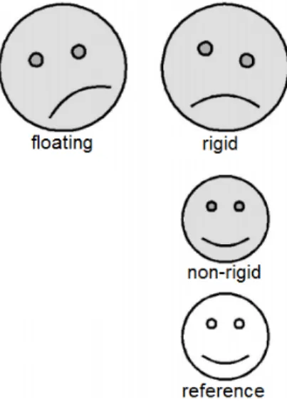
In non-rigid transformations (or deformable registrations), the transforma-tion contains localized non-rigid stretching. Deformable image registratransforma-tion (DIR) can be used in many applications once it can reproduce the non-rigid behaviour of the human body (examples: lungs and breast). It requires more complex algorithms than rigid transformation and it involves the determina-tion of a large number of parameters [29],[30]. Figure 2.3 shows the difference between rigid and non-rigid registration.

Figure 2.3: Example showing the difference between rigid and non-rigid registration. Rigid registration consists on a rigid alignment between floating and

reference images. Non-rigid registration contains non-rigid stretching and it has the same internal structure of the reference but the intensity values of the

floating image [30].

The goal in registration is to find the optimal transformation, T : (x, y, z) → (x0, y0, z0), which maps any voxel in the reference image R(x, y, z) to its corresponding voxel in the floating image F (x0, y0, z0) and so the key point is to find the following transformation [31]:

T : (x0, y0, z0) = (x, y, z) + (ux(x, y, z) + uy(x, y, z) + uz(x, y, z)) (2.3) In the above equation, we want to find the displacement vector field u(x) which can be calculated using B-Spline basis function. The displacement vector field is the vector field which includes all displacement vectors of all the voxels. Looking at figure 2.4 we can easily understand equation 2.3. It represents an example of a displacement vector field where x is a pixel

(31)

Figure 2.4: Displacement vector field [31].

in the reference image and u(x) (in red) is the displacement function. x’ represents the pixel in the floating image and it comes from adding x with u(x) (equation 2.3) [31].

2.2.1.3 B-Spline transformation

There are lots of ways to parametrise a deformable transformation. B-Spline transformation is a type of non-rigid transformations and it is popular be-cause its uses less parameters (control points) than voxels, so more efficient, but still allows for detailed deformations (how detailed depends on control point spacing) (section 2.2.1.4). It also provides some intrinsic regularisation (section 3.2.1) and it allows deformation to be easily calculated at each voxel and at any other points in the volume. Moreover, efficient implementations exist and are freely available (section 3.2.1).

2.2.1.3.1 B-Spline Curves The term B-Spline is short for basis-spline and it consists on a parametric curve of a linear combination of basis B-Splines:

u(x) =X i

(32)

Where pi is a spline coefficient and βi(x) is a piecewise spline curve [29]. B-Spline curves are used to define a continuous displacement vector field that maps the voxels in one image to those in another image [31]. In medical image registration the most common approach is to use uniform cubic B-splines curves as we can see in figure 2.5, where β(x) is a piecewise cubic polynomial and the points −2, −1, 0, +1, +2 are the control points.

Figure 2.5: B-Spline Basis Function.

Multiplying the piecewise cubic polynomial, β(x), for different scalar val-ues we obtain different curves as it is shown in figure 2.6. The notation for these scaling factors is pi and these are known for coefficient values (see equation 2.4).

Figure 2.6: B-Spline curves with different values of scaling factors.

2.2.1.4 B-Spline interpolation

Figure 2.7 represents a 2D example which shows a voxel grid aligned with an uniformly spaced control grid which divides the voxel grid into 6 × 5 tiles (in red). The displacement vector field of the pixels within a tile is influenced

(33)

by the 16 control points in the tile’s immediate vicinity [29].

Figure 2.7: A portion of 2D image showing a B-Spline control-point grid superimposed upon an aligned voxel grid [29].

A small grid is able to align small details but the process is slow and the grid is not flexible enough for large rotations and big deformations. Figure 2.8 shows a registration performed between a square and a rectangle image. After registration, the deformed grid shows the deformation between the images.

Figure 2.8: Deformed grid shows the deformation between the reference image (rectangle) and the floating image (square) [32].

Similarly, in the 3D case, the B-Spline interpolation of the x-component of the displacement vector field for a voxel located at coordinate (x, y, z)

(34)

depends on the 64 control point coefficients in the tile’s immediate vicinity and it is characterized by the following equation [29]:

ux(x, y, z) = 3 X l=0 3 X m=0 3 X n=0 βl(u)βm(v)βn(w) px,l,m,n (2.5)

px corresponds to a spline coefficient which defines the x component of the displacement vector for one of the 64 control points that influence the voxel. Positive pi means a movement to the right (vector field points to the right) and a negative pi means a movement to the left. If we do the registration of two identical images, we expect that all the coefficient values, pi, would be zero [33].

The uniform cubic B-Spline basis function βl along the x-direction is [29]:

βl(u) =                    (1 − u)3 6 : l = 0 (3u3_{− 6u}2_{+ 4)} 6 : l = 1 (−3u3+ 3u2 + 3u + 1) 6 : l = 2 u3 6 : l = 3. (2.6)

And similarly for βm and βn along the y- and z-directions, respectively [29].

Once the displacement vector field is generated, it is used to deform each voxel in the floating image. Once deformed, the floating image is compared to the reference image in terms of similarity metrics (see section 2.2.3.1.2, 3.2.1 and 3.2.1.2.2), they are what drives the registration algorithm to find the optimal result.

2.2.2 Inverse transformation models

In registration we want to find the transformation that maps the voxels of the floating image with the corresponding voxels of the reference image. The transformation tells us where any voxel of the floating image ’comes from’ in the reference image but it does not tell us where any voxel of the reference image ’goes to’ in the floating image [34]. There is no analytic solution to calculate the inverse of the transformation, T−1, however it is desirable to

(35)

know it many times, e.g. for planning tracked treatment [34], [35].

Since deformable registration methods do not compute the inverse of the interpolated transform, it is necessary to estimate it. Sections 2.2.2.1, 2.2.2.2 and 2.2.2.3 describe different methods to compute the inverse of the transformation.

2.2.2.1 Asymmetric transformation

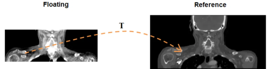
Figure 2.9 represents a schematization of a deformable registration which maps a CT image (floating) to a CBCT image (reference). In this work, we consider that the registration performed in this direction is the forward direction.

Figure 2.9: Schematization of a deformable registration performed in the forward direction which maps a CT image (floating) to a CBCT image

(reference).

Unlike forward direction, backward direction maps a CBCT image (float-ing) to a CT image (reference) as we can see in figure 2.10. In other words, swapping our reference image with our floating image, registration is per-formed in the opposite direction of the forward direction.

Asymmetric backward direction transformation is independently of the transformation in the forward direction and so it can not be consider as its inverse. It is an approach which gives us an approximation of the inverse transformation.

2.2.2.2 Symmetric inverse consistent transformation In figures 2.9 and 2.10 the transformation is optimized in the forward and backward direction, respectively. Therefore the transformation is biased towards its direction. Symmetric inverse consistent (SIC) deformable image

(36)

Figure 2.10: Schematization of a deformable registration performed in the backward direction which maps a CBCT image (floating) to a CT image

(reference).

registration is a novel technique which optimizes both forward and backward transformation by ensuring the inverse consistency criterion (see section 2.2.3.2.2) [35],[36],[37],[38].

Figure 2.11 represents a schematization of a symmetric deformable regis-tration.

Figure 2.11: Schematization of a symmetric deformable image registration which optimizes the transformation in both directions (forward and backward).

2.2.2.3 Estimating the inverse of a B-Spline transformation It is possible to estimate the inverse of a B-Spline transformation using iterative algorithms which estimate the inverse field of a displacement vector field. The algorithms compute the inverse until its achieves a desired degree of accuracy or when they reach their iteration limit (see section 3.2.1.2.3) [34].

(37)

2.2.3 Validation process: quality criteria

Validation of registration is particularly important in medical applications. Prior to clinical use it is mandatory to ensure that registration is correct and it is mapping the right voxels to the right places. Deformable image registration is not an exact science and its performance is patient-specific and also the lack of information to validate registration accuracy make a difficult task to decide whether registration is successful. Image matching quality and deformation field analysis are important steps to ensure it [39],[40],[41],[42].

2.2.3.1 Image matching quality

2.2.3.1.1 Visual assessment Visual inspection is a qualitative proce-dure of registration performance and it is an important step to registration techniques entering routine clinical use. Overlapping the reference image with the registration result is possible to infer about the image matching quality but locally implausible deformations are difficult to be detected by an expert observer [39],[41],[40]. Figures 2.12(a) and 2.12(b) represent examples of an overlap between a reference image (red) and a registration result (cyan). Registration was performed using the same reference and floating images but with different transformations and it is easy to conclude that figure 2.12(b) represents a better match than figure 2.12(a).

(a) (b)

Figure 2.12: Example of a (a) bad and (b) a good registration (red: reference image; cyan: registration result). Coronal plane images.

(38)

2.2.3.1.2 Similarity measures Similarity measure is a quantitative measure which tells us the degree of similarity between two images. There are a large number of different similarity measures and the selection of the proper measure to use depends on the images modality and the registration goal. Normalized mutual information is a very effective measure to calculate the degree of similarity between images from different modalities such as CT and CBCT [43]. Normalized cross correlation and sum of squared intensity differences work well between images from the same modality and are easy to compute [43], [27].

Normalized mutual information Mutual information (MI) mea-sures the information shared between two images and it is maximized when they are spatially aligned. It is sensitive to changes in the size of the over-lapping region therefore Studholme et al. [44] introduced the concept of normalized mutual information (NMI) which remains insensitive to changes in the size of background [45],[46]. It is given by [44]:

N M I(A, B) = H(A) + H(B)

H(A, B) (2.7)

H(A) and H(B) are the marginal entropies of image A and B, respectively, and H(A, B) the joint entropy (figure 2.13) NMI can range between 0 and 2 and values of NMI>1 typically represent a good match between images.

Figure 2.13: Representation of the entropies involved in mutual information theory [44].

The entropy H of a point in an image is a measure of how well the intensity at that point can be predicted [47]:

H(A) = −X a

(39)

H(B) = −X b

pB(b) log pB(b) (2.9) H(A, B) = −X

a,b

pAB(a, b) log pAB(a, b) (2.10) pA(a) is the probability that a point in image A has intensity a. The same theory is applicable for H(B) and H(A, B) where pAB(a, b) is the joint probability that a point in the overlap region has intensity a and b [39].

MI works well for intra- and inter-modality image registration. Different modalities may not have the same intensities but they always have mutual information in terms of spacial distributions.

Normalized cross correlation Normalized cross correlation (NCC) is given by the following equation:

N CC =

P

(i,j)∈Ω(IA(i, j) − IA)(IB(i, j) − IB) q P (i,j)∈Ω(IA(i, j) − IA)2 q P (i,j)∈Ω(IB(i, j) − IB)2 (2.11)

Where IA and IB are the intensity values of image A and B, respectively. IA and IB are the mean values of the images in the overlap region (i, j) ∈ Ω. It can takes values between -1 and +1 where +1 represents a maximum of correlation between images. NCC is very sensitive to the intensity value of a pixel therefore a small number of pixels that have large differences in intensity between images may have a big effect on the similarity measure [43].

Sum of squared intensity differences Sum of squared intensity differences (SSD) consists on one of the simplest similarity measures and the optimal transformation is found by minimizing it:

SSD = 1 N

X iA∈Ω

|A(iA) − BT(iA)|2 (2.12) Where N is the number of voxels in the overlap region Ω, A is the reference image, B is the floating image, BT is image B transformed into the coordinate space of image A and iA is a voxel in image A.

As normalized cross correlation SSD is also very sensitive to the intensity value of a voxel.

(40)

2.2.3.2 Deformation field analysis

The analysis of deformation fields enables to ensure that the deformations are physically plausible (section 2.2.3.2.1) and that forward and backward transformations are inverse-consistent (section 2.2.3.2.2).

2.2.3.2.1 Jacobian The Jacobian matrix contains 9 values (for a 3D transformation) and describes how the transformation changes in each of the 3 directions. The determinant of the Jacobian matrix (often just called the Jacobian) gives the local volume change and both can be calculated at any point in the transformation and describe the local properties of the transform at that point.

Folding occurs when the transform causes the anatomy to fold onto itself, meaning that some points in one volume now map to two points in the other volume and some points may not map to any points. To ensure that no fold-ing had occurred durfold-ing registration the transformation must be invertible, i.e., it has an inverse. The Jacobian is an indicator of the invertibility of the transformation and it is given by the following equation:

JT(x) = ∂Tx(x) dx ∂Tx(x) dy ∂Tx(x) dz ∂Ty(x) dx ∂Ty(x) dy ∂Ty(x) dz ∂Tz(x) dx ∂Tz(x) dy ∂Tz(x) dz (2.13)

JT(x) = 1 if the volume at x remains the same after the transformation, JT(x) > 1 if there is volume expansion and JT(x) < 1 if there is volume shrinkage. JT(x) ≤ 0 means that folding had occurred which is physically impossible and mathematically not invertible [44],[48].

Figure 2.14(a) shows the effect of the Jacobian in registration with a value of -35,9. It is easy to notice local foldings and twits compared with figure 2.14(b).

2.2.3.2.2 Inverse consistent error The inverse consistent (IC) error measures the degree of consistency between forward and backward transformation. Figure 2.15 represents a schematization of it where the forward transformation TF W maps the point i to j and the backward transformation TBW maps the point j to i0. The distance between i and i0 consists on the inverse consistent error: IC = ||i − i0||. The optimal transformation is found minimizing d distance.[49]

(41)

(a) (b)

Figure 2.14: Effect of the Jacobian in registration. (a) Negative Jacobian means that folding had occurred during registration. (b) Positive Jacobian means

that no folding had occurred during registration. Transversal plane images.

2.2.4 Dose comparison

Radiotherapy dose comparison plays an important rule to achieve the desired dose distribution which avoids underdosage of the target volumes (that potential increases the risk of tumour recurrence) and overdosage of normal tissues. Therefore in clinical practice it is common the comparison of two dose distributions. In sections 2.2.4.1, 2.2.4.3, 2.2.4.4 the dose comparison methods used are explained.

Figure 2.15: Schematization of the inverse consistent error: d = IC error = ||i − i0||

(42)

2.2.4.1 Relative dose difference

Relative dose difference (DD) is the most straightforward and intuitive method which consists on the difference between two dose distributions through voxel by voxel value subtraction. Given a point rr in the reference distribution and the corresponding point re in the evaluated distribution the dose difference between the two positions is De(~re) − Dr(~rr) where D represents the dose value in each point. To be able to subtract dose distributions, they must be of the same size.

In high dose gradient regions it is of less clinical significance since a large dose difference can be induced by a small alignment error [50].

A difference criterion ∆D can be set, e.g. ∆D = 3% of the maximum dose such that points with a dose difference value greater than ∆D fail this criterion and points with a dose difference value lower than ∆D pass the criterion [51].

2.2.4.2 Distance-to-agreement

Given a point in the reference distribution rr and the corresponding point re in the evaluated distribution the distance-to-agreement (DTA) corresponds to the distance between re and the closest point with the same dose value of rr in the evaluated distribution:

DT A(~rr) = min|~re− ~rr| (2.14) As with dose difference (section 2.2.4.1), a DTA criterion ∆d can be set. A threshold value of ∆d = 3mm is typically considered such that if the DTA at the comparison point is greater than ∆d the test fails and if it is lower than ∆d the test passes the criterion [51].

2.2.4.3 Gamma evaluation

The gamma test combines features of both dose difference (section 2.2.4.1) and distance-to-agreement (section 2.2.4.2) tests. It was introduced by Low et al. [52] and its evaluation complements DD and DTA tests.

Consider two 2D dose distributions, a reference Dr and an evaluated De, and its points rr and re, respectively. The gamma test is based on an

(43)

ellipsoid surface representing the acceptance criterion, e.g., ∆D = 3% of the maximum dose and ∆d = 3mm of spatial tolerance, with the center located at the reference point in question ~rr [52],[51]:

Γ(~rr, ~re) = r r2(~rr, ~re) ∆d2 + δ2(~rr, ~re) ∆D2 (2.15)

Where r(~rr, ~re) = |~re − ~rr| is the spatial difference between the posi-tion of the reference point ~rr and the position of the evaluated point ~re. δ(~rr, ~re) = De(~re) − Dr(~rr) represents the dose difference between the evalu-ate distribution Deat position ~reand the reference distribution Drat position ~

rr. A geometric representation of the ellipsoid can be found in figure 2.16 [52],[51].

Figure 2.16: Geometric representation of the gamma combined acceptance criterion of dose difference and distance-to-agreement test for 2D dose distributions. x and y axes represent the spatial location of the point in the evaluated distribution ~re relative to the point in the reference distribution ~rr (in

the center). δ axis represents the difference in dose De(~re) − Dr(~rr). In this

example point re fails the criterion (outside ellipsoid) [52],[51].

The gamma index is calculated by finding the minimum value of Γ(~rr, ~re) varying ~re:

γ(~rr) = min{Γ(~rr, ~re)}∀{~re} (2.16) Therefore the pass-fail criteria consists on:

(44)

γ(~rr) > 1, calculation fails. (2.18)

The gamma evaluation can also be applied to 3D dose distributions. For the gamma test dose distributions must have a grid resolution of 1 × 1 × 1 [52].

2.2.4.4 Dose-volume histograms

Dose distributions within a particular volume of interest (VOI) can be summarized using dose-volume histograms (DVHs) which can be of two types: differential or cumulative DVHs.

Dose bins are represented on x axis and VOI volume on y axis. First, it is defined the range of the dose bins. In a differential DVH each bin indicates the total volume of the VOI receiving a dose within a dose range of that bin [11].

The cumulative DVH represents the volume of VOI which receives a dose greater or equal to the dose indicated on the x axis. In clinical practice cumulative DVHs are more used [11].

Figure 2.17: Differential and cumulative DVHs. Two voxels are identified in the dose distribution. The one in the edge of the target volume has a lower dose than the one in the center, therefore it is represented in a low dose bin compared with the other which is represented in a high dose bin in the differential DVH. In the cumulative DVH is represented the total volume of VOI which receives a dose

(45)

2.3 Previous work

Different methods for estimating the cumulative dose received by radiother-apy patients while accounting for anatomic changes have been proposed. Yan et al. [53] using the finite element method developed a biochemical model of an elastic body to estimate organ deformations that may occurred during a radiotherapy treatment. For that purpose they used multiple daily CT images. Daily dose distributions to specific volume elements within an organ of interest were then computed while accounting for intertreatment organ deformations using registration techniques.

Rosu et al. [54] registered images between exhale and inhale images using thin-plate spline registration and dose distributions were computed for each data set. The transformation found between images was then direct applied to the exhale dose image and then they estimated the dose at the tracked position using trilinear interpolation from voxels in vicinity of the tracked voxel and, finally, the accumulated dose distributions were computed by summing the interpolation result with the original dose voxel value from the exhale data set.

Schaly et al. [55] registered multiple treatment CT studies taken throughout the treatment course to a planning CT study. Dose calculations were performed directly in the treatment studies and mapped back to the planning study using the thin-plate spline registration algorithm, allowing the fractionated dose distributions to be accumulated.

The present study makes part of a large project which has been developed between University College London (UCL) and University College London Hospital (UCLH), in order to implement adaptive radiotherapy (ART) strategies in a clinical environment for routine clinical use. ART will be a valuable tool to assist clinicians on the evaluation of off-line and online treatment procedures to account for positioning errors and anatomic changes. The work performed by Veiga et al. (submitted) studied the performance of a deformable image registration (DIR) algorithm. 5 patients with HN cancer treated with IMRT who had repeat CBCT imaging and replanning over the treatment course were studied. The software was used to deform the planning CT (pCT) scan to match a CBCT image taken before replan. Two independent tests were performed to assess registration performance: (i) features manually delineated in the CBCT by a physician were compared

(46)

with features acquired automatically by warping the pCT features with the output transformation that registers the images and (ii) comparison between dose calculations for the same IMRT plan in the deformed CT and rescan CT (rCT). Features were compared using dice similarity index (DSI), overlap index (OI), centroid position error (CoM) and distance transform (DT). Dose distributions were compared based on dose difference (DD) and gamma analysis, target coverage and dose-volume histograms (DVH).

Veiga et al. presented a proof-of-principle for the implementation of an in-house developed deformable registration to be used in ART applications and concluded that the tool will enable the implementation of an ART procedure. They showed that a pCT can be registered to a CBCT and used to produce accurate dose calculations in the space of the CBCT volume, i.e. the dose-of-the-day. In this work we investigate warping the dose-of-the-day calculations back into a common space (the pCT space) so that they can be compared to the planned dose and each other, and the cumulative dose can be calculated and used to inform planning decisions. The same software and data used by Veiga et al. are used in present study and it aims to asses registration software’s feasibility for dose remapping and summation.

(47)

Materials and methods

3.1 Data sets

This study includes data from 5 HN anonymized cancer patients provided by UCLH (Patients X, Y, Z, K and S). All the patients had significant anatomic changes during the course of the treatment which resulted in 4 of them (Patients X, Y, Z, K) being re-scanned and completely replanned. All patients underwent IMRT with a planned dose of 65Gy delivered in 30 daily fractions. The data sets consists on pCT (planning CT) images acquired as part of the standard planning process of HN cancer patients at UCLH. Each pCT had associated with it (i) a set of structures (target volumes, brainstem, spinal canal and gland parotids) that had been manually identified by an expert in HN radiotherapy imaging and (ii) the treatment plan which contains information about beams energy, number and direction. For each patient who had re-plan the CBTC image taken before it was also available. Although one of the patients has not been replanned (Patient S), important weight gain and loss were observed throughout the treatment and the weekly CBCTs images acquired during the treatment course were also available.

3.1.1 DICOM

Medical imaging data sets are in DICOM (Digital Imaging and Com-munication in Medicine) format which is the standard format between different types of medical imaging devices. DICOM RT is specified for radiotherapy modality and it includes different types of information such as: DICOM RT image includes all the images acquired during the treatment and information about their position, plane and orientation; DICOM

(48)

RT plan has all the geometric and dosimetric data relating to treatment plan (treatment beams, dose prescription, patient setup); DICOM RT dose includes dose distributions calculated from the planning system and; DICOM RT structure set includes all the structures delineated from pCT [56].

3.2 Data Processing

The study consisted of three main parts:

A. DIR to map pCT image to CBCT space and map it back to planning CT space - Performed to assess different inverse transform methods for dose summation.

B. Dose summation - Performed to compute the weekly and cumulative dose distribution received by radiotherapy patients while accounting for anatomic variations.

C. Comparison of deformed pCT dose and recalculated dose in the deformed pCT - Performed to evaluate dosimetric differences between planned and recalculated dose while accounting for anatomic variations.

Three different methods of computing the inverse of the transformation T−1 were studied and analysed (asymmetric, symmetric and estimate the inverse methods). The 4 patients who had replan were included in this study. After that, we applied the inverse transform methods for dose summation to a clinical example (patient who had no re-plan) to illustrate the delivered dose during treatment while accounting for anatomic variations. Of the 4 patients who had re-plan, 3 (Patients X, Y and Z) were con-sidered for the dosimetric comparison between planned and recalculated dose.

3.2.1 Image Registration - Performed in NifTK

Registration cases were studied and solved using NifTK (http://cmic.cs.ucl.a c.uk/home/software/) which was developed in the Centre of Medical Image Computing (CMIC) at the Department of Medical Physics and Bioengineer-ing of University College London (UCL). It contains of several tools such as NiftyView for image analysis and visualization and NiftyReg to perform

(49)

rigid and non-rigid registrations.

NifTK uses a common image format called NIfTI (neuroimaging infor-matics technology initiative) therefore NiftyView is used to convert the data sets from DICOM to NIfTI format.

Rigid registration is based on a block-matching strategy which provides a set of corresponding points between images. The process is repeated until the optimal rigid transformation is found by calculating the best correspondence between reference and floating blocks using the normalised cross correlation [57].

Deformable image registration is based on B-splines algorithm [58] to generate the displacement vector field (see section 2.2.1.3) and normalized mutual information is computed to find the best match between reference and floating image[59]:

N M I = H(R) + H(F (T ))

H(R, F (T )) (3.1)

T is the deformation which maximizes the NMI between the refer-ence R and the deformed floating F (T ) image. At first sight, we could think that maximizing the similarity would be the final goal of regis-tration. However, without any restrictions, deformations can lead to unrealistic transformation results such as folding. In order to overcome these issues two penalty terms were also considered over registration: (i) the bending energy (BE) constrains the transformation to be smooth and (ii) the Jacobian (see section 2.2.3.2.1) ensures that folding not occurred [59]. Registrations were performed with an Intel Xeon CPU E25606 (2.13GHz, 12GB RAM) with a NVIDIA Tesla C2070 GPU card (14 multiprocessors, 6GB dedicated memory).

3.2.1.1 Forward asymmetric registration

The pCT scan was set as floating image and the CBCT scan taken before replan was set as reference image. Replan was considered due to significant differences found between images to be registered therefore registration was performed in the worst case scenario.

(50)

A set of optimized registration parameters were previously optimized to suit the data sets being registered [60],[61]. The parameters include choice of the weight of the penalty terms such as bending energy and Jacobian. A rigid alignment was first applied followed by the deformable registration.

The registration process produced a new image set (deformed pCT) which has the image quality and HU of the pCT and the geometry infor-mation of the CBCT. CBCT image has a scan range smaller than the one for pCT and without any strategy deformed pCT will miss information about patient’s anatomy. Therefore prior to registration CBCT image was extended to have the same field of view of the pCT. In the extended region the transformation results of an interpolation between the initial rigid alignment and the deformation inside of the field of view of the CBCT.

Registration procedure rans in approximately 1 minute with GPU implementation.

3.2.1.2 Inverse of the transformation

Registration performed in the forward direction produced a transformation T which maps the pCT to the CBCT space. Three different methods of computing its inverse T−1 were studied. The 4 patients who had re-plan were included in this study.

3.2.1.2.1 Backward asymmetric registration Unlike forward asymmetric registration, in backward asymmetric registration the CBCT scan taken before replan was set as floating image and the pCT scan was set as reference image. The inverse rigid alignment of the forward direction was computed using NifTK and it was first applied followed by the deformable registration. Registration was performed using the same set of optimized parameters of the forward direction.

The registration process produced a new image data set (deformed CBCT) which has the image quality of the CBCT and the geometry information of the pCT.

(51)

3.2.1.2.2 Symmetric registration Symmetric registration was re-cently implemented in NifTK [38] and it optimizes forward TF W and back-ward TBW transformation (see section 2.2.2.2):

N M ISY M =

H(R) + H(F (TF W)) H(R, F (TF W)) +

H(R(TBW)) + H(F )

H(R(TBW), F ) (3.2) Where H(...) are the marginal entropies and H(..., ...) are the the joint entropies. In order order to ensure inverse consistency between transfor-mations a penalty term based on the inverse consistent error (see section 2.2.3.2.2) is also considered during registration.

The pCT scan was set as floating image and the CBCT scan taken before re-plan was set as reference image. A rigid alignment between images was first applied followed by the symmetric registration. The output were two geometrical transformations, forward and backward, and two new image data sets, one from registration performed in the forward direction (deformed pCT) and other from registration performed in the backward direction (deformed CBCT).

First, a set of registration parameters were optimized to suit the data sets being registered. The parameters studied included the weight of the bending energy and inverse-consistency penalty terms.

Symmetric registration is a time consuming process taking around 9 hours to run. It is not yet implemented on GPU and when it is it will be a lot faster, but still considerably slower than asymmetric registration as it con-siders and optimises both forward and backward transform at the same time.

3.2.1.2.3 Estimate the inverse methods - Performed in Mat-lab/NifTK Two algorithms to estimate the inverse of the forward asym-metric registration were studied and analysed:

(i) Method 1 - Developed by Jamie McClelland [34] and performed in Mat-lab.

(ii) Method 2 - Developed by Marcel Van Herk and implemented in NifTK. Method 1 finds the inverse i = T−1(r) of a point r in the reference image by an iterative process. The algorithm starts with an initial esti-mate of the inverse iest, i.e. rest = T (iest) and it computes r − rest until

(52)

the estimate is within the desired accuracy or the maximum number of iterations has been reached. Its estimates iest based on the values of the Jacobian matrix J of the transformation T which tell us how the transformation changes in each direction [34]. Although its accuracy, it consists on a far more time consuming process taking around 2/3 days to compute the inverse of each data set, since it is implemented in MAT-LAB and not in C++ it is bound to be less efficient (and so time consuming). Method 2 has the same principle as method 1 but is efficiently imple-mented. It computes the inverse in approximately 2 minutes with GPU implementation.

3.2.2 Dose Calculation - Performed in Eclipse

Varian Eclipse is a treatment planning system for external beam treatment planning.

In order to import the images in NIfTI format (section 3.2.1) to the treatment planning system they were first converted to DICOM format (section 3.1.1) using Matlab. It includes optimized functions that allow open, visualize and write NIfTI and DICOM files.

All the information about the treatment plan (based on the planning CT and developed by a radiation oncologist) is saved on a DICOM RT plan format. This file was imported to Eclipse and it was used for dose calculations in the deformed pCT. A simulated treatment was generated by applying the beam configurations of the initial plan to the anatomy of the new image registered and calculation of dose was performed (figure 3.1). Doses were calculated using a resolution of 1 mm.

This is done to calculate the dose received by the radiotherapy patient while accounting for variable anatomy. The recalculated dose was then mapped back to the planning CT dose space using three different methods of computing the inverse to study the dosimetric difference between methods.

3.2.3 Dose Summation - Performed in Matlab

We aimed to calculate the weekly and cumulative dose distributions received by the patient while accounting for anatomic variations. The method requires