Origin of atmospheric aerosols at the Pierre Auger Observatory using studies of
air mass trajectories in South America
The Pierre Auger Collaborationa, Gabriele Curcib aObservatorio Pierre Auger, Av. San Mart´ın Norte 304, 5613 Malarg¨ue, Argentina
bCETEMPS, Department of Physics, University of L’Aquila, L’Aquila, Italy
Abstract
The Pierre Auger Observatory is making significant contributions towards understanding the nature and origin of ultra-high energy cosmic rays. One of its main challenges is the monitoring of the atmosphere, both in terms of its state variables and its optical properties. The aim of this work is to analyze aerosol optical depth τa(z) values measured
from 2004 to 2012 at the observatory, which is located in a remote and relatively unstudied area of the Pampa Amarilla, Argentina. The aerosol optical depth is in average quite low – annual mean τa(3.5 km)∼0.04 – and shows a seasonal
trend with a winter minimum – τa(3.5 km)∼0.03 –, and a summer maximum – τa(3.5 km)∼0.06 –, and an unexpected
increase from August to September – τa(3.5 km) ∼ 0.055). We computed backward trajectories for the years 2005 to
2012 to interpret the air mass origin. Winter nights with low aerosol concentrations show air masses originating from the Pacific Ocean. Average concentrations are affected by continental sources (wind-blown dust and urban pollution), while the peak observed in September and October could be linked to biomass burning in the northern part of Argentina or air pollution coming from surrounding urban areas.
Keywords: cosmic ray, aerosol, air masses, atmospheric effect, HYSPLIT, GDAS. 1. Introduction
Modelling of aerosols in climate models is still a chal-lenging task, also due to the lack of a complete global coverage of long-term ground-based measurements. In South America, only few studies have been done, usu-ally located in mega-cities (Carvacho et al., 2004; L´opez et al., 2011; Morata et al., 2008; Reich et al., 2008; Zhang et al., 2012). Astrophysical observatories need a contin-uous monitoring of the atmosphere, including aerosols, and thus offer an unique opportunity to get a characteri-sation of aerosols in the same locations over several years. Here we report on seven years of aerosol optical depth measurements carried out at the Pierre Auger Observa-tory in Argentina.
The Pierre Auger Observatory is the largest operating cosmic ray observatory ever built (Abraham et al., 2004, 2010a). It is conceived to measure the flux, arrival di-rection distribution and mass composition of cosmic rays from 1018 eV to the very highest energies. It is located
in the Pampa Amarilla (35.1◦−35.5◦S, 69.0◦−69.6◦W,
and 1 300−1 700 m above sea level), close to Malarg ¨ue, Province of Mendoza. Construction was completed at the end of 2008 and data taking for the growing detec-tor array started at the beginning of 2004. The obser-vatory consists of about 1660 surface stations – water-Cherenkov tanks and their associated electronics – cov-ering an area of 3000 km2. In addition, 27 telescopes,
housed in four fluorescence detector (FD) buildings, de-tect air-fluorescence light above the array during nights with low-illuminated moon and clear optical conditions. The atmosphere is used as a giant calorimeter, represent-ing a detector volume larger than 30 000 km3. Once
cos-mic rays enter into the atmosphere, they induce exten-sive air showers of secondary particles. Charged parti-cles of the shower excite atmospheric nitrogen molecules, and these molecules then emit fluorescence light mainly in the 300−420 nm wavelength range. The number of flu-orescence photons produced is proportional to the energy deposited in the atmosphere through electromagnetic en-ergy losses undergone by the charged particles. Then, from their production point to the telescope, photons can be scattered by molecules (Rayleigh scattering) and/or at-mospheric aerosols (Mie scattering). A small component (at shorter ultra-violet wavelengths) of the fluorescence light can be absorbed by some atmospheric gases such as ozone or nitrogen dioxide.
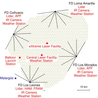
The aerosol component is the most variable term con-tributing to the atmospheric transmission function. Thus, to reduce as much as possible the systematic uncertain-ties on air shower reconstruction using the fluorescence technique, aerosols have to be continuously monitored. An extensive atmospheric monitoring system has been developed at the Pierre Auger Observatory (Abraham et al., 2010b; Louedec and Losno, 2012). The different fa-cilities and their locations are shown in Figure 1.
Ae-Preprint submitted to Atmospheric Research May 30, 2014
FD Los Leones
Lidar, HAM, FRAM IR Camera Weather Station FD Los Morados Lidar, APF IR Camera Weather Station FD Loma Amarilla Lidar IR Camera Weather Station FD Coihueco Lidar, APF IR Camera Weather Station Malargüe
Central Laser Facility Weather Station eXtreme Laser Facility Balloon
Launch Station
10 km
Figure 1: Atmospheric monitoring map of the Pierre Auger
Observa-tory (from Abraham et al. (2010b)). Gray dots indicate the positions
of surface detector (SD) stations. Black segments indicate the fields of view of the fluorescence detectors (FD) which are located in four sites, called Los Leones, Los Morados, Loma Amarilla and Coihueco, on the perimeter of the surface array. Each FD site hosts several atmospheric monitoring facilities.
rosol monitoring is performed using two central lasers (CLF / XLF) (Fick et al., 2006), four elastic scattering li-dar stations (BenZvi et al., 2007a), two aerosol phase func-tion monitors (APF) (BenZvi et al., 2007b) and two setups for the ˚Angstr¨om parameter, the Horizontal Attenuation Monitor (HAM) (BenZvi et al., 2007c) and the Photome-tric Robotic Atmospheric Monitor (FRAM) (Tr´avn´ıˇcek et al., 2007). Also, a Raman lidar is operational in-situ since June 2013. In Section 2, the measurements of the aerosol optical depth are described. The HYSPLIT air-modelling programme will be briefly described in Section 3, together with a detailed view on the air mass trajectories and ori-gin of the aerosols passing above the Pierre Auger Ob-servatory. Finally, aerosol measurements and their differ-ent features will be interpreted using backward trajecto-ries of air masses in Section 4. A preliminary version of this work was presented in Louedec et al. (2013), show-ing some links between air mass trajectories and aerosol measurements at the Pierre Auger Observatory. This pa-per provides a more complete study with the full data set available for aerosol measurements.
2. Aerosol optical depth measurements
At the Pierre Auger Observatory, several facilities have been installed to monitor the aerosol component of the at-mosphere. One of the aerosol measurements made at the observatory is the aerosol optical depth using laser tracks generated by the Central Laser Facility. This facility is operated only at nights when the observatory is taking
data: thus, aerosol data obtained are more a sampling data set than continuous measurements. The CLF is lo-cated in a position equidistant from three out of four FD sites. The main component is a laser producing a beam with a wavelength λ0fixed at 355 nm, i.e. in the middle
of the nitrogen fluorescence spectrum emitted by nitro-gen molecules excited by the passing of air showers. The pulse width of the beam is 7 ns and a maximum energy per pulse is of 7 mJ. This corresponds to the fluorescence light produced by an air shower with an energy of 1020eV
viewed from a distance of 20 km. Typically, the beam is directed vertical. When a laser shot is fired, the fluores-cence telescope detects a small fraction of the light scat-tered out of the laser beam. The recorded signal depends on the atmospheric properties. Two methods have been developed by the Auger Collaboration to estimate hourly the vertical aerosol optical depth τa(h, λ0)with the CLF,
where h is the altitude above ground level and λ0 the
CLF wavelength. Both methods assume a horizontal uni-formity for the molecular and aerosol components. The first method, the so-called ”Data Normalised Analysis”, is an iterative procedure comparing hourly average light profiles to a reference clear night where light attenuation is dominated by molecular scattering. Using a reference clear night avoids an absolute photometric calibration of the laser. About one reference clear night per year per FD site is found to be sufficient. The second method, the so-called ”Laser Simulation Analysis”, is based on the com-parison of measured laser light profiles to profiles sim-ulated with different aerosol attenuation conditions de-fined using a two-parameters model. More details can be found in Abreu et al. (2013).
The CLF provides hourly altitude profiles for each flu-orescence site during fluflu-orescence data acquisition. In Figure 2 (left), the distribution of the aerosol optical depth integrated from the ground up to 3.5 km above ground level, recorded at Los Leones, Los Morados and Coihueco is shown. Due to large distance to the CLF site, mea-surements from Loma Amarilla have not been included in this study. Only recently, data from the closer XLF have been used to measure the aerosol attenuation from Loma Amarilla (Valore et al., 2013). The mean value of
τa(3.5 km) is about 0.04. Nights with τa(3.5 km) larger
than 0.1, meaning a transmission factor lower than 90%, are rejected for air shower studies at the Pierre Auger Ob-servatory. Systematic uncertainties associated with the measurement of the aerosol optical depth are due to the relative calibration of the telescopes and the central laser, and the relative uncertainty of the determination of the reference clear profile. The total uncertainty is estimated to 0.006 for an altitude of 3.5 km above ground level. Fig-ure 2 (right) displays the monthly variation of the aero-sol optical depth integrated up to 3.5 km above ground level. The aerosol concentration depicts a seasonal trend, reaching a minimum during Austral winter and a max-imum in Austral summer. This trend is typical and has already been observed in many long-term aerosol analy-2
(3.5 km,355 nm) a τ 0 0.02 0.04 0.06 0.08 0.1 0.12 0.14 0.16 0.18 0.2 Entries 0 200 400 600 800 1000
hist
> = 0.039 a τ Los Leones < > = 0.040 a τ Los Morados < > = 0.037 a τ Coihueco < > 90 % a TQuality cut for data
Clear nights Hazy nights
hist
Month of the year
2 4 6 8 10 12 m) µ (3.5 km,355 a τ 0.01 0.02 0.03 0.04 0.05 0.06 0.07 0.08 0.09
Graph
Los Leones Los Morados CoihuecoFigure 2: Vertical aerosol optical depth measurements integrated from the ground up to 3.5 km at the fluorescence telescopes Los Leones, Los
Morados and Coihueco. (left) Distribution of aerosol optical depth values. (right) Monthly variation of mean aerosol optical depth values. Data set
between January 2004 and December 2012 in both figures. The horizontal error bars correspond to the bin size, and the vertical error bars represent the root mean square of the mean value. Colours in online version.
ses (Benavente and Acuna, 2013; Castro Videla et al., 2013; Schafer et al., 2008). Since spatial resolution in latitude and longitude for atmospheric data used by the HYSPLIT programme is one degree, only aerosol data measured at Los Morados are used since it is the closest fluorescence
145
site to the coordinates (35 S, 69 W). We subdivide the data sample into three populations:
• the clear hourly aerosol profiles with the lowest ae-rosol concentrations: ta(3.5 km)60.01 (1126
trajec-tories),
150
• the hazy hourly aerosol profiles with the highest aerosol concentrations: ta(3.5 km) > 0.10 (583
tra-jectories),
• the average hourly aerosol profiles with the aver-age aerosol concentrations: 0.03 < ta(3.5 km) 6
155
0.05 (1918 trajectories).
The relative frequencies month-by-month for clear condi-tions and hazy condicondi-tions are shown in Figure 3. Clear conditions are more common during the Austral winter than in the rest of the year. Furthermore, a clear increase
160
for the population of hazy aerosol profiles from August to September can be seen in both Figures 2 (right) and 3, contrary to the overall seasonal trend. Table 1 lists the fraction of clear and hazy aerosol profiles for each year between 2005 and 2012. For each year, the two or three
165
highest fraction values are indicated. Clear conditions are very common during Austral winter throughout all years of this analysis. The unexpected peak in hazy con-ditions during September and October is almost as stable
as the seasonal trend throughout the years, but not with 170
the same statistical significance. It could be a consequence of biomass burning in the northern part of South America or closer pollution sources coming from the larger cities San Rafael and Mendoza in the North.
3. Backward trajectory of air masses 175
After having briefly presented the air-modelling pro-gramme used in this study and checked the validity of its calculations using meteorological radio soundings, this section aims for characterising the air masses crossing over
the Pierre Auger Observatory. 180
3.1. HYSPLIT – an air-modelling programme
Different models have been developed to study air mass relationships between two regions. Among them, the HYbrid Single-Particle Lagrangian Integrated Trajectory model, or HYSPLIT (Draxler and Rolph, 2012; Rolph, 2012),185
is a commonly used air-modelling programme in atmo-spheric sciences for calculating air mass displacements from one region to another. The HYSPLIT model, devel-oped by the Air Resources Laboratory, NOAA1, is a
com-plete system designed to support a wide range of sim- 190
ulations related to regional or long-range transport and dispersion of airborne particles (Martet et al., 2009). It is possible to compute simple trajectories for complex dis-persion and deposition simulations using either puff or particle approaches within a Lagrangian framework (Cao 195
1NOAA, National Oceanic and Atmospheric Administration, U.S.A.
3
Figure 2: Vertical aerosol optical depth measurements integrated from the ground up to 3.5 km at the fluorescence telescopes Los Leones, Los
Morados and Coihueco. (left) Distribution of aerosol optical depth values. (right) Monthly variation of mean aerosol optical depth values. Data set
between January 2004 and December 2012 in both figures. The horizontal error bars correspond to the bin size, and the vertical error bars represent the root mean square of the mean value. Colours in online version.
ses (Benavente and Acuna, 2013; Castro Videla et al., 2013; Schafer et al., 2008). Since spatial resolution in latitude and longitude for atmospheric data used by the HYSPLIT programme is one degree, only aerosol data measured at Los Morados are used since it is the closest fluorescence site to the coordinates (35◦ S, 69◦ W). We subdivide the
data sample into three populations:
• the clear hourly aerosol profiles with the lowest ae-rosol concentrations: τa(3.5 km)60.01 (1126
trajec-tories),
• the hazy hourly aerosol profiles with the highest aerosol concentrations: τa(3.5 km) > 0.10 (583
tra-jectories),
• the average hourly aerosol profiles with the aver-age aerosol concentrations: 0.03 < τa(3.5 km) 6
0.05 (1918 trajectories).
The relative frequencies month-by-month for clear condi-tions and hazy condicondi-tions are shown in Figure 3. Clear conditions are more common during the Austral winter than in the rest of the year. Furthermore, a clear increase for the population of hazy aerosol profiles from August to September can be seen in both Figures 2 (right) and 3, contrary to the overall seasonal trend. Table 1 lists the fraction of clear and hazy aerosol profiles for each year between 2005 and 2012. For each year, the two or three highest fraction values are indicated. Clear conditions are very common during Austral winter throughout all years of this analysis. The unexpected peak in hazy con-ditions during September and October is almost as stable
as the seasonal trend throughout the years, but not with the same statistical significance. It could be a consequence of biomass burning in the northern part of South America or closer pollution sources coming from the larger cities San Rafael and Mendoza in the North.
3. Backward trajectory of air masses
After having briefly presented the air-modelling pro-gramme used in this study and checked the validity of its calculations using meteorological radio soundings, this section aims for characterising the air masses crossing over the Pierre Auger Observatory.
3.1. HYSPLIT – an air-modelling programme
Different models have been developed to study air mass relationships between two regions. Among them, the HYbrid Single-Particle Lagrangian Integrated Trajectory model, or HYSPLIT (Draxler and Rolph, 2012; Rolph, 2012), is a commonly used air-modelling programme in atmo-spheric sciences for calculating air mass displacements from one region to another. The HYSPLIT model, devel-oped by the Air Resources Laboratory, NOAA1, is a
com-plete system designed to support a wide range of sim-ulations related to regional or long-range transport and dispersion of airborne particles (Martet et al., 2009). It is possible to compute simple trajectories for complex dis-persion and deposition simulations using either puff or particle approaches within a Lagrangian framework (Cao
1NOAA, National Oceanic and Atmospheric Administration, U.S.A.
Year Jan Feb Mar Apr May Jun Jul Aug Sep Oct Nov Dec Clear hourly profiles
2005 –– –– –– 2%1 20%8 58% 38%7 16 5%1 21%5 4%3 4%2 11%4 2006 0%0 0%0 0%0 2%2 4%4 29% 29%33 31 4%6 14% 14%17 3 17%14 9%7 2007 0%0 0%0 3%2 31%30 10%10 54% 88%42 35 63%42 7%5 27%25 36%36 14%10 2008 20% 11%11 7 3%2 10%9 1%1 53%53 14%16 39%32 10%9 5%5 7%5 0%0 2009 4%3 2%2 0%0 0%0 21%12 53%57 20%17 11%10 4%4 22%20 17%15 3%2 2010 1%1 15%9 5%5 14%20 13%14 41% 35%34 33 4%4 0%0 1%1 0%0 8%5 2011 5%3 0%0 5%7 8%11 14%17 32% 48%34 30 27%28 3%3 0%0 7%6 8%6 2012 5%4 13%9 2%2 3%3 16%21 57% 33%59 35 15%17 0%0 8%7 0%0 7%5 All 5%22 6%27 3%18 9%76 11%87 45% 33%319 213 20%140 6%43 10%64 13%78 8%39
Hazy hourly profiles
2005 –– –– –– 0%0 0%0 0%0 0%0 0%0 4%1 0%0 6%3 14%5 2006 40%2 0%0 1%1 16%18 6%6 3%3 1%1 6%8 6%7 0%0 11%9 0%0 2007 16%11 6%3 8%5 6%6 0%0 1%1 0%0 1%1 10%7 9%8 0%0 7%5 2008 2%1 8%5 13%8 1%1 0%0 0%0 26%30 1%1 30%28 1%1 7%5 18%5 2009 38%26 9%9 21%25 2%3 0%0 4%4 20%17 5%5 9%9 0%0 3%3 12%9 2010 6%5 6%4 5%5 5%7 0%0 1%1 4%4 3%3 7%8 29%30 0%0 0%0 2011 9%6 4%4 14%19 2%3 1%1 2%2 0%0 3%3 24% 49%23 34 21%19 14%10 2012 11% 10% 11%8 7 11 14%14 1%1 0%0 4%4 6%7 15%14 6%5 21%15 0%0 All 14%59 7%32 11%74 6%52 1%8 2%11 9%56 4%28 14%97 12%78 9%54 7%34
Table 1: Fraction and statistics of aerosol hourly profiles for clear and hazy aerosol conditions for each month between 2005 and 2012. For each year, the first line gives the fraction of profiles corresponding to the aerosol conditions in the whole set of profiles recorded during the corresponding month. The second line gives the number of profiles associated to their corresponding fraction. Months without data are indicated by “–”. For each year, the two or three months with the highest fraction of clear and hazy nights are coloured in blue and red, respectively. Colours in online version.
et al., 2010; De Vito et al., 2009). In this work, HYSPLIT will be used to get backward / forward trajectories by tracking air masses backward / forward in time. The re-sulting backward / forward trajectory indicates air mass arriving at a specific time in a specific geographical lo-cation (latitude, longitude and altitude), identifying the
regions linked to it. All along the air mass paths, hourly meteorological data are used. Trajectory uncertainty for computed air masses is usually divided into three com-ponents: the physical uncertainty due to the inadequacy of the representation of the atmosphere in space and time by the model, the computational uncertainty due to numerical 4
Month of the year 1 2 3 4 5 6 7 8 9 10 11 12 0.05 0.1 0.15 0.2 0.25
hist
Clear profiles Hazy profiles Average profileshist
Figure 3: Monthly frequency over a year of clear hourly aerosol
pro-files (τa(3.5 km) 6 0.01, solid line), average hourly aerosol profiles
(0.03 < τa(3.5 km) 6 0.05, grey filled) and hazy hourly aerosol
pro-files (τa(3.5 km) >0.10, dotted line) at Los Morados. Data set between January 2005 and December 2012 is used here. Each bin is re-weighted to take into account the fact that not the same number of aerosol profiles is recorded in Winter (longer nights) or during Summer (shorter nights). Colours in online version.
uncertainties and the measurement uncertainty for the me-teorological data field in creating the model. Also, there could be sensitivity to initial conditions, especially during periods with large instabilities: for instance, estimation of the beginning of backward trajectories could be affected by very turbulent and chaotic air mass movement.
HYSPLIT provides details of some of the meteorolog-ical parameters along the trajectory. It is possible to ex-tract information on terrain height, pressure, ambient and potential temperature, rainfall, relative humidity and so-lar radiation. However, to produce a trajectory, HYSPLIT requires at least the wind vector, ambient temperature, surface pressure and height data. These data can come from different meteorological models. Among the avail-able models in HYSPLIT, the most used are the North American Meso (NAM), the NAM Data Assimilation Sys-tem (EDAS) and the Global Data Assimilation SysSys-tem (GDAS). Only the GDAS model provides meteorological data for the site of the Pierre Auger Observatory for the period starting in January 2005 and extending to the present time. The GDAS is an atmospheric model developed by the NOAA (NOAA, 2004). Those data are distributed over a one degree latitude/longitude grid (360◦×180◦), with
a temporal resolution of three hours. GDAS provides 23 pressure levels, from 1000 hPa (more or less sea level) to 20 hPa (about 26 km altitude). The data set is com-plemented by data for the surface level at the given lo-cation. The GDAS grid point most suitable for the loca-tion of the Pierre Auger Observatory is (35◦S, 69◦W), i.e.
just slightly inside the array to the north-east (Abreu et al., 2012a). Lateral homogeneity of the atmospheric vari-ables across the Auger array is assumed (Abraham et al., 2010b). Validity of GDAS data was previously studied by the Auger Collaboration: the agreement with ground-based weather station and meteorological radiosonde lau-nches has been verified. The work consisted of compar-ing the temperature, humidity and pressure values with those measured by the monitoring systems at Auger. For instance, distributions of the differences between mea-sured weather station data at the centre of the array and GDAS model data were obtained for temperature, pres-sure and water vapour prespres-sure: 1.3 K[σ=3.9 K], 0.4 hPa [σ=1.2 hPa]and−0.2 hPa[σ=2.1 hPa], respectively (Ab-reu et al., 2012a). Thanks to their highly reliable availabil-ity and high frequency of data sets, it was concluded that GDAS data could be employed as a suitable replacement for local weather data in air shower analyses of the Pierre Auger Observatory. The agreement between GDAS model and local measurements has been checked only for state variables of the atmosphere. In the next section, wind data, a key parameter in the HYSPLIT model, are tested. 3.2. Validity of the HYSPLIT calculations using
meteorologi-cal radio soundings
Above the Pierre Auger Observatory, the height de-pendent profiles have been measured using meteorolog-ical radiosondes launched mainly from the Balloon Lau-nch Station (BLS, Figure 1). The balloon flight programme was terminated in December 2010 after having been op-erated 331 times since August 2002 (Abreu et al., 2012b; Keilhauer and Will, 2012). The radiosonde records data every 20 m, approximately, up to an average altitude of 25 km above sea level, well above the fiducial volume of the fluorescence detector. The average time elapsed dur-ing its ascent was about 100 minutes on average. The measurement accuracies are 0.2◦C in temperature, 0.5−
1.0 hPa in pressure and 5% in relative humidity.
As mentioned in Section 3.1, the HYSPLIT tool requires meteorological data from the GDAS model. Using the meteorological radio soundings performed at the Pierre Auger Observatory, a balloon track is available for each flight. In Figure 4, the average-vertical profiles of wind speed for each season are displayed, as measured during balloon flights at the observatory. Each of them is com-pared to the mean vertical profile extracted from GDAS data of the corresponding season. The wind speed fluctu-ates strongly day-by-day: the largest variations are mea-sured in the Austral winter. In table 2, the mean values and the standard deviation values for the difference be-tween measured radio sounding data and GDAS data for temperature, pressure, vapour pressure and wind speed are given. Concerning the wind speed which will be of primary interest in this work, we can see that its value is slightly underestimated by the GDAS model in the lower part of the atmosphere.
Height AGL [km] 2 3 4 5 6 7 8 9 Wind speed [m/s] 0 10 20 30 40 50 Graph Winter Graph Height AGL [km] 2 3 4 5 6 7 8 9 Wind speed [m/s] 0 10 20 30 40 50 Graph Spring Graph Height AGL [km] 2 3 4 5 6 7 8 9 Wind speed [m/s] 0 10 20 30 40 50 Graph Summer Graph Height AGL [km] 2 3 4 5 6 7 8 9 Wind speed [m/s] 0 10 20 30 40 50 Graph Fall Graph
Figure 4: Seasonal vertical profiles for wind speed using the radio soundings and the GDAS model at the Malarg ¨ue location. Radio soundings data (solid line) from August 2002 to December 2010 are used: 72 profiles in winter, 95 profiles in spring, 81 profiles in summer and 81 profiles in fall. GDAS data (dashed line) from January 2005 to December 2010 are used. Each seasonal profile contains approximately 4000 profiles. The curves represent the averaged profile of wind speed for the corresponding season. The dashed bands show the distribution of 68% of the measurements. Colours in online version.
hXGDAS XRSi RMS(XGDAS XRS)
Altitude AGL [m] T [K] p [hPa] e [hPa] vw[m/s] T [K] p [hPa] e [hPa] vw[m/s]
1000 0.82 0.35 0.23 1.00 0.20 0.10 0.18 1.55
2000 0.10 0.50 0.05 0.50 0.15 0.05 0.09 1.20
4000 +0.50 0.20 +0.02 1.30 0.10 0.03 0.02 1.75
6000 +0.08 0.02 +0.05 +1.40 0.07 0.02 0.01 2.84
8000 +0.20 +0.01 +0.02 +2.50 0.08 0.02 0.02 3.45
Table 2: Mean and standard deviation values for the differences between measured radio sounding (RS) data and GDAS model data. Values calculated for different probed altitudes. T: temperature, p: pressure, e: vapour pressure, vw: wind speed. Data sets from January 2005 to December 2010.
6
Figure 4: Seasonal vertical profiles for wind speed using the radio soundings and the GDAS model at the Malarg ¨ue location. Radio soundings data (solid line) from August 2002 to December 2010 are used: 72 profiles in winter, 95 profiles in spring, 81 profiles in summer and 81 profiles in fall. GDAS data (dashed line) from January 2005 to December 2010 are used. Each seasonal profile contains approximately 4000 profiles. The curves represent the averaged profile of wind speed for the corresponding season. The dashed bands show the distribution of 68% of the measurements. Colours in online version.
hXGDAS−XRSi RMS(XGDAS−XRS)
Altitude AGL [m] T [K] p [hPa] e [hPa] vw[m/s] T [K] p [hPa] e [hPa] vw[m/s]
1000 −0.82 −0.35 −0.23 −1.00 0.20 0.10 0.18 1.55
2000 −0.10 −0.50 −0.05 −0.50 0.15 0.05 0.09 1.20
4000 +0.50 −0.20 +0.02 −1.30 0.10 0.03 0.02 1.75
6000 +0.08 −0.02 +0.05 +1.40 0.07 0.02 0.01 2.84
8000 +0.20 +0.01 +0.02 +2.50 0.08 0.02 0.02 3.45
Table 2: Mean and standard deviation values for the differences between measured radio sounding (RS) data and GDAS model data. Values calculated for different probed altitudes. T: temperature, p: pressure, e: vapour pressure, vw: wind speed. Data sets from January 2005 to December 2010.
X position wrt starting point [km]
-40 -20 0 20 40 60 80 100 120 140
Y position wrt starting point [km]
-100 -80 -60 -40 -20 0 20 40 60 80 100
histoTRAJ
histoTRAJ
-0.6 -0.4 -0.2 0 0.2 0.4 0.6 -0.6 -0.4 -0.2 0 0.2 0.4 0.6Graph
N S E W NE SE SW NWFigure 5: Distribution of trajectories and direction of balloon flights
at the Pierre Auger Observatory. Balloon data set from August 2002 to
December 2010. (top) Distribution of balloon trajectories with a start lo-cation fixed at(0, 0)and represented by a star. All the altitudes probed during the flight are integrated in this histogram. Colours indicate the frequency of a region, from red (more likely) to blue (less likely). (bot-tom) Directions of balloon flights are given in dashed line. Directions of air masses starting at 500 m above the observatory location (35 S, 69 W) using HYSPLIT are plotted in solid line for the year 2008. Colours in online version.
since a change in direction is not common for air mass tra-jectories at these probed altitudes, an agreement of direc-tions along this short path can be extrapolated to larger distances travelled by air masses. Thus, after these two crosschecks, i.e. the vertical profiles for wind speed and
315
the directions of air masses travelling above the Auger array, it can be concluded that air mass calculations for
Figure 6: Example of a back trajectory from the Malarg ¨ue location
us-ing HYSPLIT. The initial height is fixed at 500 m above ground level for
the red line, 1000 m for the blue line and 3000 m for the green line (map taken from Google Earth). Colours in online version.
the location (35 S, 69 W) are suitable. This conclusion complements the analysis and results of the former study of GDAS data for the Pierre Auger Observatory (Abreu et 320
al. (2012a)).
3.3. Origin and trajectories of air masses arriving at the Pierre Auger Observatory
The trajectories of air masses arriving at the Auger Observatory have been evaluated for four years (2007– 325
2010). In this way, the seasonal variations in the origin of air masses can be shown in the analysis. A 48-h back-ward trajectory is computed every hour, throughout the years. Also, the evolution profiles of the different mete-orological quantities can be estimated and recorded. The 330
key input parameters for the runs are given in Table 3. In Figure 6, an example of a 48-h backward trajectory from HYSPLIT is shown for altitudes fixed at 500 m, 1000 m or 3000 m above the Malarg ¨ue location. A 2-day time scale is a good compromise with respect to aerosol lifetime, air 335
mass dispersion and computing time. Each run provides the geographical location of air mass trajectories (arriv-ing at different altitudes) at the Auger Observatory and the evolution (along the trajectories) of the relevant mete-orological physical parameters (temperature, relative hu- 340
midity, etc). Some geographical locations of air masses show significant changes of direction during the previ-ous 48 hours. Two different methods have been used to display air mass origin and mean trajectory.
The first visualisation is a two-dimensional diagram, 345
longitude versus latitude. From this display, it is possible to extract regional influence on air quality at the Auger site. Also, changes in direction are obvious. Therefore all regions that an air mass path traversed during its entire 7
Figure 5: Distribution of trajectories and direction of balloon flights
at the Pierre Auger Observatory. Balloon data set from August 2002 to
December 2010. (top) Distribution of balloon trajectories with a start lo-cation fixed at(0, 0)and represented by a star. All the altitudes probed during the flight are integrated in this histogram. Colours indicate the frequency of a region, from red (more likely) to blue (less likely). (bot-tom) Directions of balloon flights are given in dashed line. Directions of air masses starting at 500 m above the observatory location (35◦S, 69◦
W) using HYSPLIT are plotted in solid line for the year 2008. Colours in online version.
To validate the wind directions used in HYSPLIT cal-culations, the agreement between the directions of the bal-loon flights and the directions of air mass paths estimated using HYSPLIT is checked. In Figure 5 (top), the distri-bution of balloon trajectories obtained at the Auger site is given. In this plot, the altitude evolution through the flight is not indicated. The corresponding directions of
Figure 6: Example of a back trajectory from the Malarg ¨ue location
us-ing HYSPLIT. The initial height is fixed at 500 m above ground level for
the red line, 1000 m for the blue line and 3000 m for the green line (map taken from Google Earth). Colours in online version.
these balloon trajectories are given in blue in Figure 5 (bot-tom), tending roughly to a South-East direction (detailed explanations on how to obtain this plot are given in Sect. 3.3, where the steps here are given by the different data points recorded during the balloon flight). To exclude altitudes too much higher than the 500 m AGL computed by HYS-PLIT, only the first 20 min of each flight is used to estimate the direction of a radio sounding. On the other hand, using the HYSPLIT tool, 48-h forward trajectories from an altitude fixed at 500 m are computed every hour, for the year 2008. Following the same method as the one ex-plained in Sect. 3.3, the resulting distribution of air mass directions is plotted in red. The distributions for different initial altitudes will be shown later in Figure 8. Air mass directions are just slightly dependent on the altitude. The agreement between balloon trajectories and forward tra-jectories computed by HYSPLIT is once again very good: since a change in direction is not common for air mass tra-jectories at these probed altitudes, an agreement of direc-tions along this short path can be extrapolated to larger distances travelled by air masses. Thus, after these two crosschecks, i.e. the vertical profiles for wind speed and the directions of air masses travelling above the Auger array, it can be concluded that air mass calculations for the location (35◦ S, 69◦W) are suitable. This conclusion
complements the analysis and results of the former study of GDAS data for the Pierre Auger Observatory (Abreu et al., 2012a).
3.3. Origin and trajectories of air masses arriving at the Pierre Auger Observatory
The trajectories of air masses arriving at the Auger Observatory have been evaluated for eight years (2005– 7
Parameter Setting
Meteorological dataset GDAS
Trajectory direction Backward / Forward
Trajectory duration 48 hours
Start point Auger Observatory (35◦S, 69◦W)
Start height 500 m / 1000 m AGL
Vertical motion Model vertical velocity
Table 3: Input parameters used for all HYSPLIT runs.
2012). In this way, the seasonal variations in the origin of air masses can be shown by the analysis. A 48-h back-ward trajectory is computed every hour, throughout the years. Also, the evolution profiles of the different mete-orological quantities can be estimated and recorded. The key input parameters for the runs are given in Table 3. In Figure 6, an example of a 48-h backward trajectory from HYSPLIT is shown for altitudes fixed at 500 m, 1000 m or 3000 m above the Malarg ¨ue location. A 2-day time scale is a good compromise with respect to aerosol lifetime, air mass dispersion and computing time. Each run provides the geographical location of air mass trajectories (arriv-ing at different altitudes) at the Auger Observatory and the evolution (along the trajectories) of the relevant mete-orological physical parameters (temperature, relative hu-midity, etc). Some geographical locations of air masses show significant changes of direction during the previ-ous 48 hours. Two different methods have been used to display air mass origin and mean trajectory.
The first visualisation is a two-dimensional diagram, longitude versus latitude. From this display, it is possible to extract regional influence on air quality at the Auger site. Also, changes in direction are obvious. Therefore all regions that an air mass path traversed during its entire 48-h travel period towards the Pierre Auger Observatory are displayed. In Figure 7, the distribution of the back-ward trajectories for each month during the year 2008 is displayed, for a start altitude fixed at 500 m above ground level at the observatory. Also the fluctuations change month-by-month: e.g., June or August are months where the air masses show large fluctuations trajectory-to-trajectory. These two months are exactly the ones having the highest fractions of clear profiles for this year in Table 1.
Another visualisation of the trajectory is done using the direction of the air mass paths: it consists of subdivid-ing each air mass trajectory into two 24-h sub-trajectories. The direction for the most recent sub-trajectory is then chosen among these directions: North/N (0◦±22.5◦),
North-East / NE (45◦±22.5◦), East / E (90◦±22.5◦), South-East
/ SE (135◦±22.5◦), South / S (180◦±22.5◦), South-West
/ SW (225◦±22.5◦), West / W (270◦±22.5◦), North-West
/ NW (315◦±22.5◦) – origin of the frame being fixed at
the Pierre Auger Observatory. For each trajectory, its ori-gin is obtained as follows: using the angle between two steps along the trajectory, a sub-direction is defined for
each step (i.e. 24 in our case) and then the global direction corresponds to the most probable value of sub-directions for the whole sub-path. The different directions recorded are then plotted in a histogram. In Figure 8, these polar histograms are shown for each month of the year 2008. The polar histograms are normalised to one, i.e. the sum of the height entries corresponding to the height direc-tions is equal to one. Most of the months have air mas-ses with a North-West origin. Air masmas-ses coming from the East are particularly rare. The observations remain the same when the start altitude of the backward trajec-tories is modified. For the highest initial altitude (1000 m above ground level at the observatory), the fluctuations trajectory-to-trajectory are larger and the air masses travel faster; their endpoint is farther from the Pierre Auger Ob-servatory.
4. Interpretation of aerosol measurements using back-ward trajectories of air masses
As described in Section 2, aerosol concentrations mea-sured at the Pierre Auger Observatory can fluctuate stron-gly night-by-night. Nevertheless, a seasonal trend with a minimum in Austral winter is found. The computed HYSPLIT trajectories are given in Figure 9 (top) for the conditions described in Section 2 (clear, hazy and average hourly aerosol profiles). During clear conditions, the air masses come mainly from the Pacific Ocean as already ob-served in Allen et al. (2011). For hazy conditions, these air masses travel principally through continental areas dur-ing the previous 48 hours. Followdur-ing the conclusion of a chemical aerosol analysis performed at the Auger site by Micheletti et al. (2012), NaCl crystals are detected in aerosol samplings during Austral winter, the period with mostly clear conditions and trajectories pointing back to the Pacific Ocean. Thus, these NaCl crystals could come from the Pacific Ocean, even if we cannot exclude another main origin as salt flats as main origin. Snow is another phenomenon that has to be taken into account here. As explained in Micheletti et al. (2012), even though snow-falls are quite rare during winter in this region, the low temperatures conserve the snow on ground for long peri-ods. An aerosol source (soil) blocked by snow, combined with air masses coming from Pacific Ocean, are probably 8
Longitude [degree] -90 -85 -80 -75 -70 -65 -60 -55 -50 -45 Latitude [degree] -50 -45 -40 -35 -30 -25 histoTRAJ Pacific Ocean South America Atlantic Ocean January 2008 histoTRAJ Longitude [degree] -90 -85 -80 -75 -70 -65 -60 -55 -50 -45 Latitude [degree] -50 -45 -40 -35 -30 -25 histoTRAJ Pacific Ocean South America Atlantic Ocean February 2008 histoTRAJ Longitude [degree] -90 -85 -80 -75 -70 -65 -60 -55 -50 -45 Latitude [degree] -50 -45 -40 -35 -30 -25 histoTRAJ Pacific Ocean South America Atlantic Ocean March 2008 histoTRAJ Longitude [degree] -90 -85 -80 -75 -70 -65 -60 -55 -50 -45 Latitude [degree] -50 -45 -40 -35 -30 -25 histoTRAJ Pacific Ocean South America Atlantic Ocean April 2008 histoTRAJ Longitude [degree] -90 -85 -80 -75 -70 -65 -60 -55 -50 -45 Latitude [degree] -50 -45 -40 -35 -30 -25 histoTRAJ Pacific Ocean South America Atlantic Ocean May 2008 histoTRAJ Longitude [degree] -90 -85 -80 -75 -70 -65 -60 -55 -50 -45 Latitude [degree] -50 -45 -40 -35 -30 -25 histoTRAJ Pacific Ocean South America Atlantic Ocean June 2008 histoTRAJ Longitude [degree] -90 -85 -80 -75 -70 -65 -60 -55 -50 -45 Latitude [degree] -50 -45 -40 -35 -30 -25 histoTRAJ Pacific Ocean South America Atlantic Ocean July 2008 histoTRAJ Longitude [degree] -90 -85 -80 -75 -70 -65 -60 -55 -50 -45 Latitude [degree] -50 -45 -40 -35 -30 -25 histoTRAJ Pacific Ocean South America Atlantic Ocean August 2008 histoTRAJ Longitude [degree] -90 -85 -80 -75 -70 -65 -60 -55 -50 -45 Latitude [degree] -50 -45 -40 -35 -30 -25 histoTRAJ Pacific Ocean South America Atlantic Ocean September 2008 histoTRAJ Longitude [degree] -90 -85 -80 -75 -70 -65 -60 -55 -50 -45 Latitude [degree] -50 -45 -40 -35 -30 -25 histoTRAJ Pacific Ocean South America Atlantic Ocean October 2008 histoTRAJ Longitude [degree] -90 -85 -80 -75 -70 -65 -60 -55 -50 -45 Latitude [degree] -50 -45 -40 -35 -30 -25 histoTRAJ Pacific Ocean South America Atlantic Ocean November 2008 histoTRAJ Longitude [degree] -90 -85 -80 -75 -70 -65 -60 -55 -50 -45 Latitude [degree] -50 -45 -40 -35 -30 -25 histoTRAJ Pacific Ocean South America Atlantic Ocean December 2008 histoTRAJ
Figure 7: Distribution of 48-h backward trajectories from the Malarg ¨ue region by month. Paths estimated with HYSPLIT for the year 2008, for a start a start altitude fixed at 500 m AGL. The black star represents the Pierre Auger Observatory. The black line represents the South American coast. Colours indicate the frequency of a region, from red (more likely) to blue (less likely). Colours in online version.
9
Figure 7: Distribution of 48-h backward trajectories from the Malarg ¨ue region by month. Paths estimated with HYSPLIT for the year 2008, for a start altitude fixed at 500 m AGL. The black star represents the Pierre Auger Observatory. The black line represents the South American coast. Colours indicate the frequency of a region, from red (more likely) to blue (less likely). Colours in online version.
-0.6 -0.4 -0.2 0 0.2 0.4 0.6 -0.6 -0.4 -0.2 0 0.2 0.4 0.6 Graph N S E W NE SE SW NW January 2008 Graph -0.6 -0.4 -0.2 0 0.2 0.4 0.6 -0.6 -0.4 -0.2 0 0.2 0.4 0.6 Graph N S E W NE SE SW NW February 2008 Graph -0.6 -0.4 -0.2 0 0.2 0.4 0.6 -0.6 -0.4 -0.2 0 0.2 0.4 0.6 Graph N S E W NE SE SW NW March 2008 Graph -0.6 -0.4 -0.2 0 0.2 0.4 0.6 -0.6 -0.4 -0.2 0 0.2 0.4 0.6 Graph N S E W NE SE SW NW April 2008 Graph -0.6 -0.4 -0.2 0 0.2 0.4 0.6 -0.6 -0.4 -0.2 0 0.2 0.4 0.6 Graph N S E W NE SE SW NW May 2008 Graph -0.6 -0.4 -0.2 0 0.2 0.4 0.6 -0.6 -0.4 -0.2 0 0.2 0.4 0.6 Graph N S E W NE SE SW NW June 2008 Graph -0.6 -0.4 -0.2 0 0.2 0.4 0.6 -0.6 -0.4 -0.2 0 0.2 0.4 0.6 Graph N S E W NE SE SW NW July 2008 Graph -0.6 -0.4 -0.2 0 0.2 0.4 0.6 -0.6 -0.4 -0.2 0 0.2 0.4 0.6 Graph N S E W NE SE SW NW August 2008 Graph -0.6 -0.4 -0.2 0 0.2 0.4 0.6 -0.6 -0.4 -0.2 0 0.2 0.4 0.6 Graph N S E W NE SE SW NW September 2008 Graph -0.6 -0.4 -0.2 0 0.2 0.4 0.6 -0.6 -0.4 -0.2 0 0.2 0.4 0.6 Graph N S E W NE SE SW NW October 2008 Graph -0.6 -0.4 -0.2 0 0.2 0.4 0.6 -0.6 -0.4 -0.2 0 0.2 0.4 0.6 Graph N S E W NE SE SW NW November 2008 Graph -0.6 -0.4 -0.2 0 0.2 0.4 0.6 -0.6 -0.4 -0.2 0 0.2 0.4 0.6 Graph N S E W NE SE SW NW December 2008 Graph
Figure 8: Direction of air masses influencing the Auger atmosphere for each month. Direction of trajectories estimated using HYSPLIT for the year 2008, with input parameters given in Table 3, at two different start altitudes: 500 m AGL (solid line) and 1000 m AGL (dashed line). Each distribution is normalised to one. Colours in online version.
10
Figure 8: Direction of air masses influencing the Auger atmosphere for each month. Direction of trajectories estimated using HYSPLIT for the year 2008, with input parameters given in Table 3, at two different start altitudes: 500 m AGL (solid line) and 1000 m AGL (dashed line). Each distribution is normalised to one. Colours in online version.
Longitude [degree] -90 -85 -80 -75 -70 -65 -60 -55 Latitude [degree] -50 -45 -40 -35 -30 -25 histoTRAJ Pacific Ocean South America Atlantic Ocean 0.01 ≤ (3.5 km) a τ ≤ Distribution of trajectories: 0.00 histoTRAJ Longitude [degree] -90 -85 -80 -75 -70 -65 -60 -55 Latitude [degree] -50 -45 -40 -35 -30 -25 histoTRAJ Pacific Ocean South America Atlantic Ocean 0.05 ≤ (3.5 km) a τ ≤ Distribution of trajectories: 0.03 histoTRAJ Longitude [degree] -90 -85 -80 -75 -70 -65 -60 -55 Latitude [degree] -50 -45 -40 -35 -30 -25 histoTRAJ Pacific Ocean South America Atlantic Ocean 0.30 ≤ (3.5 km) a τ ≤ Distribution of trajectories: 0.10 histoTRAJ -0.6 -0.4 -0.2 0 0.2 0.4 0.6 -0.6 -0.4 -0.2 0 0.2 0.4 0.6 Graph N S E W NE SE SW NW 0.01 ≤ (3.5 km) a τ ≤ Air mass path directions: 0.00
Graph -0.6 -0.4 -0.2 0 0.2 0.4 0.6 -0.6 -0.4 -0.2 0 0.2 0.4 0.6 Graph N S E W NE SE SW NW 0.05 ≤ (3.5 km) a τ ≤ Air mass path directions: 0.03
Graph -0.6 -0.4 -0.2 0 0.2 0.4 0.6 -0.6 -0.4 -0.2 0 0.2 0.4 0.6 Graph N S E W NE SE SW NW 0.30 ≤ (3.5 km) a τ ≤ Air mass path directions: 0.10
Graph
Figure 9: Distribution of backward trajectories and direction of air masses for clear, average and hazy aerosol conditions. Paths estimated with HYSPLIT for the years between 2005 and 2012 and aerosol optical depth data coming from the CLF measurements. (top) Distribution of 48-h backward trajectories from the Malarg ¨ue location for a start altitude fixed at 500 m AGL. Colours indicate the frequency of a region, from red (more likely) to blue (less likely). (bottom) Direction of trajectories with input parameters given in Table 3, at two different start altitudes AGL: 500 m (solid line) and 1000 m (dashed line). Each distribution is normalised to one. Colours in online version.
the main causes for these clear nights observed in winter at the Pierre Auger Observatory.
The direction of air masses for clear, average and hazy
420
aerosol conditions are presented in Figure 9 (bottom) for two different start altitudes at the location of the obser-vatory: 500 m AGL (solid line) and 1000 m AGL (dashed line). The same conclusions can be drawn for both initial altitudes. Nevertheless, a slight shift to the West is seen
425
for the highest altitude for hazy aerosol conditions. To relativise this disagreement, it seems important to note that atmospheric aerosols are usually located in the low part of the atmosphere, typically in the first 2 km. Hazy aerosol profiles are dominated by winds coming from the
430
North-East (especially at low start altitude), typical in Sep-tember/October, just after the Austral winter and its cor-responding air masses coming from the Pacific Ocean. Such an observation of an increase in the aerosol optical depth values from August to September, combined with
435
air masses coming from the North-East, could indicate a relationship to pollution emitted by surrounding urban areas (e.g. San Rafael or Mendoza) or the phenomenon of biomass burning in the northern part of Argentina or Bolivia. It is now well-known that wildfire emissions in
440
South America, mainly in Brazil, Argentina, Bolivia or
Paraguay, occurring during the dry season, strongly af-fect a vast part of the atmosphere in South America via long-term transportation of air masses (Andreae et al., 2001; Fiebig et al., 2009; Freitas et al., 2005; Ulke et al., 445
2011). Locally, aerosol optical depth values are usually 10 to 20 times greater than in months without burning biomass. An analysis done by Castro Videla et al. (2013) shows that the mean number of fires reaches a peak from August to October in the northern part of South America 450
(0 S to 30 S in latitude). This fire activity could corre-spond to the peak observed in aerosol concentration at the Pierre Auger Observatory. However, without a more complex modelling of air masses, only hints can be given to explain this high fraction of hazy conditions in Sep- 455
tember and a more quantitative assessment of the link source/receptor would require further analysis.
5. Conclusion
A better understanding of air mass behaviour affect-ing the Pierre Auger Observatory has been realised by 460
applying the HYSPLIT tool that tracks air masses from one region to another. Air masses above the observatory 11
Figure 9: Distribution of backward trajectories and direction of air masses for clear, average and hazy aerosol conditions. Paths estimated with HYSPLIT for the years between 2005 and 2012 and aerosol optical depth data coming from the CLF measurements. (top) Distribution of 48-h backward trajectories from the Malarg ¨ue location for a start altitude fixed at 500 m AGL. Colours indicate the frequency of a region, from red (more likely) to blue (less likely). (bottom) Direction of trajectories with input parameters given in Table 3, at two different start altitudes AGL: 500 m (solid line) and 1000 m (dashed line). Each distribution is normalised to one. Colours in online version.
the main causes for these clear nights observed in winter at the Pierre Auger Observatory.
The direction of air masses for clear, average and hazy aerosol conditions are presented in Figure 9 (bottom) for two different start altitudes at the location of the obser-vatory: 500 m AGL (solid line) and 1000 m AGL (dashed line). The same conclusions can be drawn for both initial altitudes. Nevertheless, a slight shift to the West is seen for the highest altitude for hazy aerosol conditions. To relativise this disagreement, it seems important to note that atmospheric aerosols are usually located in the low part of the atmosphere, typically in the first 2 km. Hazy aerosol profiles are dominated by winds coming from the North-East (especially at low start altitude), typical in Sep-tember/October, just after the Austral winter and its cor-responding air masses coming from the Pacific Ocean. Such an observation of an increase in the aerosol optical depth values from August to September, combined with air masses coming from the North-East, could indicate a relationship to pollution emitted by surrounding urban areas (e.g. San Rafael or Mendoza) or the phenomenon of biomass burning in the northern part of Argentina or Bolivia. It is now well-known that wildfire emissions in South America, mainly in Brazil, Argentina, Bolivia or
Paraguay, occurring during the dry season, strongly af-fect a vast part of the atmosphere in South America via long-term transportation of air masses (Andreae et al., 2001; Fiebig et al., 2009; Freitas et al., 2005; Ulke et al., 2011). Locally, aerosol optical depth values are usually 10 to 20 times greater than in months without burning biomass. An analysis done by Castro Videla et al. (2013) shows that the mean number of fires reaches a peak from August to October in the northern part of South America (0◦ S to 30◦ S in latitude). This fire activity could
corre-spond to the peak observed in aerosol concentration at the Pierre Auger Observatory. However, without a more complex modelling of air masses, only hints can be given to explain this high fraction of hazy conditions in Sep-tember and a more quantitative assessment of the link source/receptor would require further analysis.
5. Conclusion
A better understanding of air mass behaviour affect-ing the Pierre Auger Observatory has been realised by applying the HYSPLIT tool that tracks air masses from one region to another. Air masses above the observatory 11
do not have the same origin throughout the year. Ae-rosol concentrations measured at the observatory depict two notable features: a seasonal trend with a minimum reached in Austral winter, and a quick increase occurring yearly just after August. The first can be explained by air masses transported from the Pacific Ocean and trav-elling above snowy soils to the observatory. The peak in September and October could be interpreted as air mass transport from biomass burning occurring in the northern of South America (mainly in the northern of Argentina and Bolivia) during dry season. However, another cause such as air pollution transported from closer urban ar-eas, also located to the north of the observatory, cannot be excluded. Future studies that include satellite data or ground-level monitoring between the observatory and possible pollution source regions could resolve this issue. However, for both cases, air mass transport plays a key role in the aerosol component present above the Pierre Auger Observatory.
6. Acknowledgments
The successful installation, commissioning, and oper-ation of the Pierre Auger Observatory would not have been possible without the strong commitment and effort from the technical and administrative staff in Malarg ¨ue. G. Curci was supported by the Italian Space Agency (ASI) in the frame of PRIMES project.
We are very grateful to the following agencies and organizations for financial support: Comisi´on Na-cional de Energ´ıa At´omica, Fundaci´on Antorchas, Gob-ierno De La Provincia de Mendoza, Municipalidad de Malarg ¨ue, NDM Holdings and Valle Las Le ˜nas, in grat-itude for their continuing cooperation over land ac-cess, Argentina; the Australian Research Council; Con-selho Nacional de Desenvolvimento Cient´ıfico e Tec-nol´ogico (CNPq), Financiadora de Estudos e Projetos (FINEP), Fundac¸˜ao de Amparo `a Pesquisa do Estado de Rio de Janeiro (FAPERJ), S˜ao Paulo Research Foun-dation (FAPESP) Grants #2010/07359-6, #1999/05404-3, Minist´erio de Ciˆencia e Tecnologia (MCT), Brazil; AVCR, MSMT-CR LG13007, 7AMB12AR013, MSM0021620859, and TACR TA01010517 , Czech Republic; Centre de Calcul IN2P3/CNRS, Centre National de la Recherche Scientifique (CNRS), Conseil R´egional Ile-de-France, D´epartement Physique Nucl´eaire et Corpusculaire (PNC-IN2P3/CNRS), D´epartement Sciences de l’Univers (SDU-INSU/CNRS), France; Bundesministerium f ¨ur Bildung und Forschung (BMBF), Deutsche Forschungsgemein-schaft (DFG), Finanzministerium Baden-W ¨urttemberg, Helmholtz-Gemeinschaft Deutscher Forschungszentren (HGF), Ministerium f ¨ur Wissenschaft und Forschung, Nordrhein-Westfalen, Ministerium f ¨ur Wissenschaft, Forschung und Kunst, Baden-W ¨urttemberg, Germany; Istituto Nazionale di Fisica Nucleare (INFN), Ministero dell’Istruzione, dell’Universit`a e della Ricerca (MIUR), Gran Sasso Center for Astroparticle Physics (CFA),
CETEMPS Center of Excellence, Italy; Consejo Nacional de Ciencia y Tecnolog´ıa (CONACYT), Mexico; Minis-terie van Onderwijs, Cultuur en Wetenschap, Neder-landse Organisatie voor Wetenschappelijk Onderzoek (NWO), Stichting voor Fundamenteel Onderzoek der Materie (FOM), Netherlands; Ministry of Science and Higher Education, Grant Nos. N N202 200239 and N N202 207238, The National Centre for Research and De-velopment Grant No ERA-NET-ASPERA/02/11, Poland; Portuguese national funds and FEDER funds within COMPETE - Programa Operacional Factores de Com-petitividade through Fundac¸˜ao para a Ciˆencia e a Tec-nologia, Portugal; Romanian Authority for Scientific Research ANCS, CNDI-UEFISCDI partnership projects nr.20/2012 and nr.194/2012, project nr.1/ASPERA2/2012 ERA-NET, PD-2011-3-0145-17, and PN-II-RU-PD-2011-3-0062, Romania; Ministry for Higher Edu-cation, Science, and Technology, Slovenian Research Agency, Slovenia; Comunidad de Madrid, FEDER funds, Ministerio de Ciencia e Innovaci´on and Consolider-Ingenio 2010 (CPAN), Xunta de Galicia, Spain; The Leverhulme Foundation, Science and Technology Fa-cilities Council, United Kingdom; Department of En-ergy, Contract Nos. DE-AC02-07CH11359, DE-FR02-04ER41300, DE-FG02-99ER41107, National Science Foun-dation, Grant No. 0450696, 0855680, 1207605, The Grainger Foundation USA; NAFOSTED, Vietnam; Marie Curie-IRSES/EPLANET, European Particle Physics Latin American Network, European Union 7th Framework Program, Grant No. PIRSES-2009-GA-246806; and UN-ESCO.
Appendix A. Supplementary data
Supplementary data to this article can be found on-line.
References
Abraham, J., et al., 2004. Properties and performances of the prototype instrument for the Pierre Auger Observatory. Nucl. Instrum. Meth. A
523, 50–95.
Abraham, J., et al., 2010. The fluorescence detector of the Pierre Auger Observatory. Nucl. Instrum. Meth. A 620, 227–251.
Abraham, J., et al., 2010. A study of the effect of molecular and aerosol conditions in the atmosphere on air fluorescence measurements at the Pierre Auger Observatory. Astropart. Phys. 33, 108–129. Abreu, P., et al., 2012. Description of atmospheric conditions at the
Pierre Auger Observatory using the Global Data Assimilation Sys-tem (GDAS). Astropart. Phys. 35, 591–607.
Abreu, P., et al., 2012. The rapid atmospheric monitoring system of the Pierre Auger Observatory. JINST 7, P09001.
Abreu, P., et al., 2013. Techniques for measuring aerosol attenuation us-ing the Central Laser Facility at the Pierre Auger Observatory. JINST
8, P04009.
Abbasi, R., et al., 2006. Techniques for measuring atmospheric aerosols at the high resolution Fly’s Eye experiment. Astropart. Phys. 25, 74– 83.
Allen, G., et al., 2011. South East Pacific atmospheric composition and variability sampled along 20◦during VOCALS-REx. Atmos. Chem.
Phys. 11, 5237–5262.
Andreae, M.O., et al., 2001. Transport of biomass burning smoke to the upper troposphere by deep convection in the equatorial region. Geo-phys. Res. Lett. 28, 951–954.
Benavente, N.R. and Acuna, J.R., 2013. Study of the dynamics of the aerosol optical depth in South America from MODIS images of Terra and Aqua satellites (2000–2012). AIP Conf. Proc. 1527, 625–628. BenZvi, S., et al., 2007. The lidar system of the Pierre Auger Observatory.
Nucl. Instrum. Meth. A 574, 171–184.
BenZvi, S., et al., 2007. Measurement of the aerosol phase function at the Pierre Auger Observatory. Astropart. Phys. 28, 312–320.
BenZvi, S. for the Pierre Auger Collaboration, 2007. Measurement of aerosols at the Pierre Auger Observatory. Proc. 30th ICRC, M´erida, M´exico 4, arXiv:0706.3236, 355–358.
Cao, X., Roy, G. and Andrews, W.S., 2010. Modelling the concentra-tion distribuconcentra-tions of aerosol puffs using articial neural networks. Boundary-Layer Meteorol. 136, 83–103.
Carvacho, O.F., et al., 2004. Elemental composition of springtime aerosol in Chill´an, Chile. Atmos. Env. 38, 5349–5352.
Castro Videla, F., et al., 2013. The relative role of Amazonian and non-Amazonian fires in building up the aerosol optical depth in South America: a five year study (2005–2009). Atmos. Res. 122, 298–309. De Vito, T.J., et al., 2009. Modelling aerosol concentration distributions
from transient (puff) sources. Can J. Civ. Eng. 36, 911–922.
Draxler, R.R. and Rolph, G.D., 2013. HYSPLIT (HYbrid Single-Particle Lagrangian Integrated Trajectory). Model access via NOAA ARL READY website (http://www.arl.noaa.gov/HYSPLIT.php) NOAA Air Resources Laboratory, College Park, MD.
Fick, B., et al., 2006. The Central Laser Facility at the Pierre Auger Ob-servatory. JINST 1, P11003.
Fiebig, M., Lunder, C.R. and Stohl, A., 2009. Tracing biomass burning ae-rosol from South America to Troll Research Station, Antarctica. Geo-phys. Res. Lett. 36, L14815.
Freitas, S.R., et al., 2005. Monitoring the transport of biomass burning emissions in South America. Environ. Fluid Mech. 5, 135–167. Keilhauer, B. and Will, M., for the Pierre Auger Collaboration, 2012.
De-scription of atmospheric conditions at the Pierre Auger Observatory using meteorological measurements and models. Eur. Phys. J. Plus
127, 96.
Khain, A.P., 2009. Notes on state-of-the-art investigations of aerosol ef-fects on precipitation: a critical review. Environ. Res. Lett. 4, 015004– 015023.
L´opez, M.L., et al., 2011. Elemental concentration and source identifi-cation of PM10 and PM2.5 by SR-XRF in C´ordoba City, Argentina. Atmos. Env. 45, 5450–5457.
Louedec, K. for the Pierre Auger Collaboration, 2011. Atmospheric mon-itoring at the Pierre Auger Observatory – Status and Update. Proc. 32nd ICRC, Beijing, China 2, arXiv:1107.4807, 63–66.
Louedec, K. for the Pierre Auger Collaboration, 2013. Origin of atmo-spheric aerosols at the Pierre Auger Observatory using backward tra-jectory of air masses. J. Phys. Conf. Ser. 409, 012236.
Louedec, K. for the Pierre Auger Collaboration, and Losno, R., 2012. Atmospheric aerosols at the Pierre Auger Observatory and environ-mental implications. Eur. Phys. J. Plus 127, 97.
Martet, M., et al., 2009. Evaluation of long-range transport and deposi-tion of desert dust with the CTM MOCAGE. Tellus 61B, 449–463. Micheletti, M.I., et al., 2012. Elemental analysis of aerosols collected at
the Pierre Auger South Cosmic Ray Observatory with PIXE tech-nique complemented with SEM/EDX. Nucl. Instrum. Meth. B 288, 10–17.
Morata, D., et al., 2008. Characterisation of aerosol from Santiago, Chile: an integrated PIXE-SEM-EDX study. Environ. Geol. 56, 81–95. Nilsson, E.D., et al., 2001. Effects of air masses and synoptic weather
on aerosol formation in the continental boundary layer. Tellus 53B, 462–478.
NOAA Air Resources Laboratory (ARL), 2004. Global Data As-similation System (GDAS1) archive information, tech. report (http://ready.arl.noaa.gov/gdas1.php).
Reich, S., et al., 2008. Air pollution sources of PM10 in Buenos Aires City. Environ. Monit. Assess. 155, 191–204.
Rolph, G.D., 2013. Real-time Environmental Applications and Display sYstem (READY). (http://www.ready.arl.noaa.gov) NOAA Air
Re-sources Laboratory, College Park, MD.
Schafer, J.S., et al., 2008. Characterization of the optical properties of atmospheric aerosols in Amazˆonia from long-term AERONET moni-toring (1993–1995 and 1999–2006). J. Geophys. Res. 113, D04204. Tr´avn´ıˇcek, P. for the Pierre Auger Collaboration, 2007. New method
for atmospheric calibration at the Pierre Auger Observatory using FRAM, a robotic astronomical telescope. Proc. 30th ICRC, M´erida, M´exico 4, arXiv:0706.1710, 347–350.
Ulke, A.G., Longo, K.M. and Freitas, S.R., 2011. Biomass burning in South America: transport patterns and impacts, Biomass-Detection, ISBN: 978–953–307–492–4.
Valore, L. for the Pierre Auger Collaboration, 2013. Measuring atmo-spheric aerosol attenuation at the Pierre Auger Observatory. Proc. 33rd ICRC, Rio de Janeiro, Brasil, arXiv:1307.5059, 100–103.
Zhang, Y., et al., 2012. Aerosol daytime variations over North and South America derived from multiyear AERONET measurements. J. Geo-phys. Res. 117, D05211.