ii
THE ASYMMETRIC EFFECTS OF INTEREST RATE CHANGES ON HOUSEHOLD CONSUMPTION: A CASE FOR SOUTH AFRICA
Siphosethu Lucia Fikizolo
How household consumption reacts to
changes in the interest rate
Dissertation presented as the partial requirement for
obtaining a Master's degree in Statistics and Information
Management
i NOVA Information Management School Instituto Superior de Estatística e Gestão de Informação Universidade Nova de Lisboa
THE ASYMMETRIC EFFECTS OF INTEREST RATE CHANGES ON HOUSEHOLD
CONSUMPTION: A CASE FOR SOUTH AFRICA
HOW HOUSEHOLD CONSUMPTION REACTS TO CHANGES
IN THE INTEREST RATE
Siphosethu Lucia Fikizolo
Dissertation presented as the partial requirement for obtaining a Master's degree in Statistics and Information Management, Specialization in Information Analysis and Management
Advisor / Co‐supervisor: Jorge Morais Mendes March 2020
2
Table of Contents
Abstract ... 4
List of abbreviations and acronyms ... 5
1.1. Background of the study ... 6
1.2. Problem statement ... 7
1.3. Research purpose ... 8
1.4. Research aims and objectives ... 8
1.5. Research hypothesis ... 8
1.6. Methodology ... 9
1.7. Organizational structure of the paper ... 9
2.1 Introduction ... 10
2.2 Theoretical literature ... 10
2.2.1 Review of theories on consumption ... 10
2.2.2 Review of theories on interest rates ... 12
2.3 Empirical review ... 14
2.4 Assessment of literature ... 17
2.5 Conclusion ... 17
3.1 Introduction ... 18
3.2 Data type and sources ... 18
3.3 Model specification ... 18
3.4 Definition and measurement of variables in the model ... 22
3.5 Data Analysis ... 23
3.5.1 Stationarity test ... 23
3.5.2 Cointegration test and the long run relationship ... 23
3.5.3 Heteroscedasticity ... 24
3.5.4 Autocorrelation test ... 24
4.1 Introduction ... 25
4.2 Data analysis results ... 25
4.2.1 Results of the unit root test ... 25
4.2.2 Heteroscedasticity results ... 27
3
4.3 Does repo rate impact consumption spending in the short run? ... 28
4.4 Cointegration test and the long run relationship ... 30
4.5 Results of the estimated long run equation ... 31
4.6 Evidence of sign asymmetry test ... 32
4.7 Robustness test results ... 34
4.8 Evidence of Size asymmetry ... 36
5.1 Introduction ... 39
5.2 Summary of findings ... 39
5.3 Policy implications and recommendations ... 40
5.4 Practical limitations of the study and areas for further research ... 41
5.5 Conclusion ... 41
Bibliography ... 43
List of figures Figure 4.1: Autocorrelation function (ACF) ... 28
Figure 4.2: Responses of growth in real consumption expenditure to positive repo rate changes ... 29
Figure 4.3: Size asymmetry results for repo rate loosening shocks... 37
Figure 4.4: Size asymmetry results for repo rate tightening shocks ... 38
List of tables Table 4.1: Stationarity results of the Augmented Dickey-Fuller test ... 26
Table 4.2 Heteroscedasticity results of the Koenker Basset test (KB) ... 27
Table 4.3: Cointegration results ... 30
Table 4.4: Results of the estimated long run equation ... 31
Table 4.5: Regression results testing for sign asymmetry results ... 33
Table 4.6: Robustness test results of equation (3.7) ... 35
4
Abstract
This paper examines the effect of positive and negative interest rate changes on Household final consumption expenditure. That is to what extent do positive and negative interest rate changes impact consumption spending in South Africa? Is there significant evidence of asymmetric effects? Data for South Africa is used to test the theory in the South African context. Through the study, an increase in interest rates is expected to have a negative effect on household consumption.
Key words:
GDP, monetary policy, interest rates, repo rate, asymmetry, household consumption expenditure, VAR
5
List of abbreviations and acronyms
ADF Augmented Dickey-Fuller ARDL Autoregressive Distributed lad CPI Consumer Price Index
ECM Error Correction Model SARB South African Reserve Bank MPC Monetary Policy Committee GDP Gross Domestic Product
OECD Organisation for Economic Co-operation and Development OLS Ordinary Least Squares
CCEM Common Correlation Effects Mean SVAR Structural Vector Auto Regression PCE Private Consumption Expenditure
6
CHAPTER ONE
INTRODUCTION AND BACKGROUND OF THE STUDY
1.1. Background of the study
Subsequent to exchange controls, the South African Reserve Bank (SARB) adopted an inflation rate targeting policy from year 2000. The SARB has used the repo rate as the policy instrument to control the level of inflation and contain it within the target range of three to six percent. The Bank’s mandate then became the pursuit of low and non-volatile inflation as well as the protection of the domestic currency (the Rand). The effectiveness of the repurchase rate (repo rate) as a policy instrument to control the level of inflation has been widely criticised not only in the South African context but also internationally. A variety of research has been conducted on the effect of the instrument or rather monetary policy on different macroeconomic variables.
The monetary policy committee (MPC) of the SARB is responsible for monetary policy decisions, which in the case of South Africa is changing the official rate, the repo rate. Changes in the repo rate are manifested in changes in various interest rates. When the MPC decides on the direction of the official rate, it sets in motion a series of economic events. The sequence of events kicks off with the initial effect on financial markets, which then affects current expenditure levels. Mollentze (2012) stipulates that changes in domestic demand have an impact on current production levels, wages and employment, and thereby influence the inflation rate. This is referred to as the transmission mechanism of monetary policy.
The monetary policy transmission mechanism is one of the most prominent mechanisms in an economy as it reflects the process through which monetary policy decisions are transmitted to growth in real gross domestic product (GDP), inflation and other macroeconomic variables. A change in the repo rate causes changes in other short-term money-market rates of money-market instruments with different maturities and interbank deposits. Preceding a repo rate change are instant changes on banks’ interest rates almost immediately, affecting the interest rates banks charge
7
their customers as well as what they pay to savers and thus the cost of capital and consumer spending.
In proving the practicality of the monetary policy transmission mechanism, a lot of research has been conducted and most of it focused on the effect of monetary policy on economic growth as well as on the different components of GDP. Household final consumption expenditure accounts for 61 percent of GDP in South Africa, it is therefore of interest to know how it responds to monetary policy. This paper zooms in to one of the elements of the Keynesian growth model, consumption, by investigating the effects of changes in interest rates on Household final consumption expenditure.
1.2. Problem statement
Kahneman and Tversky (1979) in their influential work on how has come to be known as behavioural finance offered the concept of prospect theory. This theory suggests that individuals are afraid of losses and rather prefer gains. This is manifested in a utility function that is that is concave in gains and convex in losses. It is reasonable to expect that such preferences would suggest consumption behaviour of the Duesenberry (1949) type, where the consumption function is steeper for increases in wealth but flatter for wealth reductions. This is the well-known Ratchet effect in consumption. Deducing from these rationales, it makes sense to expect that increases in in wealth may lead to higher consumption but a fall in wealth may lead to a smaller reduction in consumption in absolute terms.
This argument introduces the possibility of asymmetry in the consumption-wealth channel of monetary policy transmission. Lower interest rates lead to higher wealth which can be used by households to finance higher consumption through equity withdrawals, higher mortgage or increased willingness to spend in general. Conversely, higher interest rates lead to lower wealth which may not proportionately reduce consumption due to the prospect theory and ratchet effect arguments. Put differently, interest rate changes inversely affect asset value, which may have asymmetric effects on consumption at least in the short to medium term.
This study assesses the presence of asymmetric effects based on the size and sign of interest rate shocks. Hence, the study examines these two aspects. In determining
8
the sign asymmetry, the study determines if there are differential effects of positive and negative interest rate changes on household consumption? Secondly, is there asymmetry based on the size of interest rate changes on household consumption? That is, does the one, two, three and four standard deviation increases in interest rate have different effects on the consumption spending?
1.3. Research purpose
The purpose of this paper is to determine if there are asymmetric effects between positive and negative interest rate changes on consumption spending. Furthermore, the findings of this paper will inform policy makers of how the fluctuations in interest rates affect households in the South African economy.
1.4. Research aims and objectives
The study aims to investigate the impact of interest rate changes on households’ consumption in the South African economy.
The objectives of the study are:
To determine whether the effect of interest rates on Household final consumption expenditure differ when during monetary policy tightening from those during monetary policy loosening periods and
To measure the magnitude by which interest rates affect household consumption.
1.5. Research hypothesis
The study will test the following hypothesis:
There is a significant and negative relationship between interest rates and household consumption.
This simply put as the null and alternative hypotheses becomes:
H0: There are significant asymmetric effects between monetary policy tightening and
9
H1: There are no significant asymmetric effects between monetary policy tightening
and loosening effects on consumption spending
1.6. Methodology
By applying the Ordinary Least squares as well as the Vector Autoregressive approach, the study empirically investigates the asymmetric effects of interest rate changes on Household final consumption expenditure in South Africa. In order to test for the unit root properties of the data, the Augmented Dickey-Fuller (ADF) test is used. The study further uses the Johansen approach in order to test cointegration.
1.7. Organizational structure of the thesis
The study consists of six chapters, starting with chapter one, which gives the background of the study. Chapter two presents an overview of the study followed by chapter three which gives the literature review.
Following chapter three is chapter four in which the methodology to be used in the study is presented. Chapter five gives the analytical technique and interpretation of results with chapter six presenting the conclusion, policy recommendations and limitations of the study.
10
CHAPTER TWO LITERATURE REVIEW
2.1 Introduction
This chapter provides the theoretical framework of the study along with the empirical theory. The theoretical literature serves as a platform for the conceptual framework of the study and enables proper policy recommendations. The empirical literature is used to explore the work done by other researchers, the different methods employed and in order to determine whether there exists a gap in literature. The chapter is divided into two sections. The first section deals with theoretical literature and the last section deals with empirical literature.
2.2 Theoretical literature
This section reviews the theories that deal with consumption as well as interest rates. The first part of this section looks to consumption theories while its second and last part reflects on interest rate theories.
2.2.1 Review of theories on consumption
Over the years, consumption theories have been developed to explain the basis of consumption. The first consumption theory developed was Keynes’s General Theory. Keynes simplified consumption and his methodology included neither abstract, mathematical theory nor detailed econometrics. He relied on intuition and was of the argument that people would increase their consumption as their income increases.
Keynes’s basic model of consumption was that current consumption expenditures are driven by current income. The Keynesian consumption function is usually written as:
𝐶𝑡 = 𝑎 + 𝑏𝑌𝑡 , (𝑎 > 0, 0 < 𝑏 < 1)
where 𝐶𝑡 represents consumption at period t, 𝑎 is autonomous consumption ( the
11
consume (MPC), and 𝑌𝑡 is disposable income at period t. Initial linear econometric
consumption functions estimated by ordinary least squares (OLS) produces results that conformed to Keynes’s theory in that consumption seemed to be closely related to current disposable income and the MPC seemed to be positive and less than one. The first critique to Keyne’s general theory was Nobel-laureate Trygve Haavelmo who pointed out the bias that is present in OLS estimation when income is correlated with the error term. Upon that, the corrected estimates of the MPC turned out to be considerably lower than OLS estimates. About the same time, Simon Kuznets refines the national account measures of income and consumption and pointed out a paradox that could not be explained by the simple linear consumption function. The Kuznets paradox was that the percentage of disposable income that is consumed is remarkably constant in the long run, which suggests a proportional consumption function, implying that the intercept tern a is equal to zero. However, short-run aggregate time-series estimates on income and consumption consistently produced estimates that showed 𝑎>0, which implied that the share of income consumed declines as income rises.
Explaining the Kuznets paradox became a primary goal for consumption theorists in the 1950s. An early approach was the relative income hypothesis, which extended the Keynesian general theory by adding past income levels and the income of other households. The relative income hypothesis mainly reflected that households’ consumption depends not only on the current income but also on current income relative to past income levels and relative to the income of other households.
Two other theories pioneered by Nobel laureates, the life cycle model associated with Franco Modiagliani and the permanent-income hypothesis developed by Milton Friedman, were easier to reconcile with foundations of consumer choice and became modern consumption theories. The two theories differed mainly in that the life-style theory emphasised natural variations in earnings over a finite lifetime whereas the permanent-income model stressed general variations in income over an indefinite horizon.
Irving Fisher used the framework of the model based on intertemporal utility maximisation in his theory of interest in the 1920s. Modern macroeconomists have extended the basic theory in various ways. One of the truly modern extensions of the
12
theory is the application of dynamic mathematical methods to the problem of utility maximisation. A second major innovation is the modelling of uncertainty and expectations in a rigorous way. Finally, modern macro-econometricians have devised ingenious ways of testing the validity of intertemporal utility maximisation theory.
2.2.2 Review of theories on interest rates
Interest on money measures the marginal preference for holding cash in hand over cash for deferred delivery. The rate at which deferred cash earnings are measured is then the interest rate. In simple terms, an interest rate is the charge of borrowing money or the reimbursement for the service and risk of lending money. Since interest rate is the cot to the borrower and return to the lender, it affects the borrowing and lending, investment and saving, portfolio composition, selection of projects types, capital-intensity of production techniques chosen, international capital flows, income distribution and a lot of other macroeconomic variables.
A lot of theories have been put in place in an attempt to explain the origin of interest rates, their impact on other economic variables as well as their generation. This study focuses on the three main theories of interest rates determination: the Classical, loanable funds and the Keynesian theories.
The classical theory
The classical theory of interest compares the supply of savings with the demand for borrowing (investment). With the use of the supply and demand curves, the equilibrium rate is determined as the point at which the two curves cross. The aggregate saving is the gap between the total national income and the total consumption expenditure. Given the current income, there is a natural tendency for economic units to spend that income on present consumption. To economic units, money now is valued more than money next year. This preference necessitates a reward to induce various economic units to save. This reward is referred to as the interest rate. The existence of time preference requires that greater savings necessitate higher rate of interest.
On the demand side, firms and other economic units demand capital to make profits by producing goods. The investment takes place because economic units expect to
13
maximise future consumption by investing in roundabout methods of production now. The classical view regards interest as determined by the productivity of capital goods providing the main elements of demand and the willingness to save. The rate of interest determined in this sense is often referred to as the natural rate or the classical real rate.
The Loanable funds theory
The loanable funds theory extends the classical theory by adding monetary and non-monetary factors. In the loanable funds theory, the interest rate is determined as the rate at which the demand and supply for money are equal. The theory is cantered under the assumptions that the market for loanable funds is fully integrated and characterised by perfect mobility of funds across markets and that there is perfect competition. In the loanable funds theory, the demand for loanable funds originates from domestic businesses, consumers, governments and foreign borrowers while the supply is generated from savings, dispersion of money in the banking system and foreign lending. With these factors determining long term interest rates, short term interest rates are decided by financial and monetary conditions in the economy.
The Keynesian theory/ Liquidity preference theory
Keynes describes the liquidity preference theory in terms of three motives that determine the demand for liquidity: the transactions motive, the precautionary motive and the speculative motive. The transactions motive states that economic units have a preference for liquidity in order to guarantee having sufficient cash on hand for basic day-to-day needs.
The precautionary motive relates to individuals’ preference for additional liquidity in the event that an unexpected problem or cost arises that requires a substantial outlay of cash. The speculative motive refers to investors’ general reluctance to commit to tying up investment capital in the present for fear of missing out on a better opportunity in the future.
The liquidity preference theory then suggests that economic units demands a higher interest rate on assets with long maturities as they would have rather preferred cash or other highly liquid holdings. Interest rates on short term securities are lower due to their high liquidity.
14
2.3 Empirical review
Exploring the linkage between wealth effects, arising stock and housing, market channels for 11 advanced countries, Coskun et al (2018) employed regression analysis through the common correlated effects mean group (CCEM) estimator , the Durbin-Hausman cointegration and Duminitrescuu and Hurlin (2013) causality tests. Their findings were that consumption is mostly explained by income and housing wealth is positively and significantly correlated with consumption. They also detected a negative linage between consumption and stock wealth. Their results also suggested a long run cointegration relationship among consumption, income, interest rates, housing wealth, and stock wealth. Moreover, their results implied that housing wealth, rather than stock wealth, is the primary source of consumption growth in advanced countries.
McDonald et al. (2011), examined the role of the consumption-wealth channel in explaining asymmetric effects of monetary policy changes. Their study made use of the structural vector autoregressive model (SVAR) to test the importance of the wealth channel on consumption. In doing so, five variables were used, namely: inflation, income, consumption, wealth and the interest rate. The model was further used as a benchmark model to trace the impulse response of consumption to an interest rate shock. The findings of the study were that shocks to wealth have a positive impact on consumption. Secondly, turning off the wealth effects makes a significant difference to the response of consumption to shocks to interest rates. Furthermore, the asymmetry in the consumption-wealth channel suggested that the central bank should take cognizance of the fact that monetary tightening will not reign in consumption growth to the desired extent, especially during periods when wealth is growing strong.
Examining the extent to which dynamic international general equilibrium model can account for observed movements in real interest rates and interest rate differentials for Group seven countries, Begum (1998) found that measured real interest rates are countercyclical in a single country and that the contemporaneous cross-corrections between international real interest differentials and output growth spreads are negative.
15
Uncovering the relationship between real interest rates and economic growth, Hansen & Seshadri (2013) analysed the long-span data on real interest rates and productivity growth with the focus on estimating their long-run correlation. They found that real interest rate is mildly countercyclical with their best estimate of long-run correlation being 0.20. The authors argue that a negative correlation reduces the variability in the stochastic intervals.
Exploring the long-term determinants of interest rates and the relationship between variations in interest rates and the rate of economic growth, Bosworth (2012) found a positive correlation between interest rates and the rate of economic growth. Data from various large economies were used to demonstrate the influence of foreign interest rates in an increasingly globalized world capital market.
A method was developed to adjust both long and short-term interest rates for expected inflation. The paper suggests that capital markets are highly integrated at the global level and that it makes little sense to model, analyse, or forecast interest rates within a closed-economy framework. Furthermore, there was only a weak relationship between real interest rates and economic growth.
Araujo (2017) examined the relationship between GDP growth and economic variables that could possibly affect it. Such variables included interest rates, unemployment, labour, labour force participation rates, shadow interest rates, stock market performance and bond market performance. In examining such a relationship, regressions were run on time series data collected from the economies and central banks of the United States, European Union and Japan. There was no statistically significant relationship between interest rates and GDP growth as well as positive values for the interest rate coefficients for two out of three regressions. Urbanovsky (2017) investigated relationships between selected macroeconomic variables: interest rate, price level, money supply and real GDP in the Czech Republic Two implemented vector autoregression models with different lag length reached slightly different conclusions. VAR(1) suggests that three pairs of Granger causality exist, in particular between price level and interest rate, between real GDP and interest rate and between real GDP and price level.
16
VAR (2) uncovered two more pairs of Granger causality between money supply and interest rate and between money supply and price level. Despite better prediction power of VAR(2) in case of money supply, low correlation coefficient comprising variable money supply raises doubts about Both VARs also agreed that interest rate could be changed by change of price level and that interest rate could be changed by change of real GDP. These conclusions represented potential recommendations to macroeconomic policy authorities.
Investigating the relationship between interest rates and economic growth in Nigeria, Obumuyi (2009) used time series analysis and annual data from 1970 to 2006. In the study, the co-integration and error correction model were used to capture both long-run and short-long-run dynamics of the variables in the model. The empirical results indicate that real lending rates have significant effect on economic growth. The study further concluded that there also exists a unique long-run relationship between economic growth and its determinants, including interest rates.
The results imply that the behaviour of interest rate is important for economic growth in view of that the relationship between interest rates and investment as well as investment and growth.
In an attempt to investigate whether interest rate triggers capital formation, Dutta et.al. (2017) built a multivariate framework by constructing a model of capital formation, interest rate and GDP growth rate and employed ARDL bounds test in addition to Johansen Maximum likelihood procedure. The study found that there exists unidirectional reserve casualty on interest by Capital formation and GDP. In examining the impact of monetary policy on private capital formation in South Africa, Khumalo (2014) used an Autoregressive Distributed lag (ARDL) - ECM procedure to run cointegration tests among variables. The study’s findings were that there exists a long run relationship among the variables included and most importantly that interest rate exerts a significant and negative impact on South Africa’s capital formation.
Vengel (2015) used Consumer Expenditure Survey data along with state base Mortgage Interest Rate Survey data to estimate the relationship between interest rates and Household final consumption expenditure in the United States. The
17
analysis showed a slight but significant positive correlation suggesting that households contracted their spending when interest rates went down.
Inspired by the change in Indian banking legislation, which encouraged banks to offer higher interest rate deposits to citizens above sixty years, Kapoor and Ravi (2009) examined the effect of interest rates on household consumption. They used consumption data from the Indian National Sample Survey to calculate regression discontinuity estimates based on age cut-offs.
Kapoor and Ravi’s findings indicated a negative relationship between interest rates and Household final consumption expenditure. Furthermore, the authors highlighted that a 50 basis points increase in interest rates on deposits leads to an immediate decline of consumption expenditure by 12 percent.
Investigating the effect of interest rates on deposit on Household consumption in Ghana et al. (2014) used the ARDL Bound test to test cointegration among variables and found that there exists a significant negative relationship between interest rate on deposits and Household final consumption expenditure short run.
2.4 Assessment of literature
The hypothesis of the study is drawn from the traditional Keynesian theory of consumption. Most empirical evidence seems to support its postulations. The foundation of the study is built from the work of Macdonald et al (2011). Macdonald et al (2011) examined the role of the consumption-wealth channel in explaining asymmetric effects of monetary policy changes. This study then investigates the asymmetric effects of monetary policy, through repo rate changes, on Household final consumption expenditure.
2.5 Conclusion
This chapter represented the theoretical literature on household consumption, interest rate determination and the link between interest rates and consumption. The second part of the study reviewed empirical studies conducted by previous researchers on topics similar to the study. Most of the studies were a guideline in building the model used in this study and the hypothesis thereon.
18
CHAPTER THREE
RESEARCH METHODOLOGY
3.1 Introduction
This chapter represents the analytical techniques used in this study in order to examine the asymmetric effects of repo rate changes on Household final consumption expenditure in South Africa. The chapter includes the type and sources of data used for the study, the specification of the model used in the study, research techniques as well as diagnostic tests employed in the study.
3.2 Data type and sources
The study used quarterly series for the period 2000 quarter one to 2018 quarter two obtained from published sources. Data is extracted from two main sources; Statistics South Africa and the South African reserve Bank. All estimations as well as the various econometric tests were carried out using Rats and E-views software’s.
3.3 Model specification
The Keynesian absolute income hypothesis specified a consumption function as: 𝐶𝑡 = 𝑎 + 𝑏𝑌𝑡 ……… (3.1)
Where 𝑌𝑡 is income at period t. For this study, the Keynesian model is extended to accommodate other variables that might influence consumption. The consumption function is therefore specified as:
𝐶𝑡 = 𝑓(𝑌, 𝑅) ……….. (3.2)
To test for robustness, the following model is used.
19
Where:
𝐶𝑡 is Household final consumption expenditure at period t, 𝑌 is disposable income, A
is assets, D is debt, R is the interest rate and Ir is the inflation rate. Three methodologies are to be used in this analysis
Method 1: A Vector Autoregressive method (VAR) to get impulse responses (the
dynamic path followed by consumption after an unexpected increase in the interest rate)
A Vector Autoregressive method (VAR) is to be used in order to assess the role of interest rate changes on household consumption. The VAR model is estimated using Choleski ordering. Consumption is placed before interest rates. This suggests interest rate response contemporaneously to consumption. P denotes the number of lags used in the estimation. This will be selected using various statistical criteria such as Akaike information criterion or Schwarz Bayesian criteria. In addition, to test robustness of the effect of interest rate, I also estimate the VAR model with variables in levels rather than as growth rates. This will capture any existing cointegration relationships. The VAR model using variables in growth rates requires variables to be stationary. Whereas the model using variables in levels requires the variables to be integrated order one I(1).
𝐶𝑡= 𝑏20+ ∑ 𝑏21, 𝑝 𝑖=1 𝑅𝑡−𝑖+ ∑ 𝑏22, 𝑝 𝑖=1 𝐶𝑡−𝑖+ 𝑒2,𝑡 ………… (3.4) 𝑅𝑡 = 𝑏10+ ∑ 𝑏11 𝑝 𝑖=1 , 𝑅𝑡−𝑖+ ∑ 𝑏12 , 𝑝 𝑖=1 𝐶𝑡−𝑖+ 𝑒1,𝑡
Where 𝑅𝑡 denotes the percentage change in interest rates (repo rate), 𝐶𝑡 is
Household final consumption expenditure, and 𝑒𝑡∼ (0, ∑) is uncorrelated white
20
Method 2: Linear regressions approach to determine both long run and short run
relationships as well as sign asymmetry (the impact or the coefficients)
Cointegration tests are to be conducted in order to identify any long-run relationships between the variables. The Johansen cointegration approach will be used through which the Maximum Eigen value and the Trace statistic are to be used to determine the cointegration relationship. After having identified the existence of the cointegration relationship, the study proceeds to estimate the long-run relationship and determine the speed of adjustment. The speed of adjustment shows the magnitude of returning to equilibrium after having deviated from equilibrium. This will also reveal the duration over which disequilibrium will be corrected. The estimated long-run equation is given by equation (3.5). All variables should be integrated order one I(1).
𝐶𝑡 = 𝛽0+ 𝛽1 𝑌𝑡+ 𝛽2𝑅𝑡+ 𝛽3𝐶𝑟𝑖𝑠𝑑𝑢𝑚𝑡+ 𝑒𝑡……… (3.5)
where 𝑒𝑡 is the error term.
Since this paper focuses on the potential asymmetric effects of interest rates changes on household consumption, ∆𝑅𝑡+ and 𝑅
𝑡− are defined such that the changes
in interest rates are split between periods when the repo rate is increased and periods when it is decreased. The short run equation is estimated using equation (3.6) below and this includes the determination of the asymmetric effects of interest rate changes. The 𝑒𝑐𝑡 captures the error correction term which measures the speed of correction required in returning to equilibrium state after a disequilibrium state. The speed of adjustment is required to have a negative sign and should be statistically significant in order to indicate gradual return to equilibrium post deviation ∆𝐶𝑡 = 𝛽0+ 𝑑1 𝑒𝑐𝑡𝑡−1+ 𝛽1 ∆𝑌𝑡+ 𝛽3𝐶𝑟𝑖𝑠𝑑𝑢𝑚𝑡+ 𝛽4∆𝑅𝑡++ 𝛽6𝑅𝑡−+ 𝑒𝑡……… (3.6)
To capture robustness in the results obtained from equation (3.6) above, equations (3.7) and (3.8) are used
∆𝐶𝑡 = 𝛽0+ 𝑑1 𝑒𝑐𝑡𝑡−1+ 𝛽1 ∆𝑌𝑡+ 𝛽3𝐶𝑟𝑖𝑠𝑑𝑢𝑚𝑡+ 𝛽2∆𝐶𝑡−1+ 𝛽4∆𝑅𝑡++ 𝛽
6𝑅𝑡−+ 𝑒𝑡 ... (3.7)
∆𝐶𝑡 = 𝛽0+ 𝑑1 𝑒𝑐𝑡𝑡−1+ 𝛽1 ∆𝑌𝑡+ 𝛽3𝐶𝑟𝑖𝑠𝑑𝑢𝑚𝑡+ 𝛽2∆𝐶𝑡−1+ 𝛽3 ∆𝐶𝑡−2+ 𝛽4∆𝑅𝑡++
21
Asymmetry is tested by determining whether 𝛽4 = 𝛽6 in equation (3.6). Rejecting the
equality in these coefficients implies that there is asymmetry. This means positive interest rate changes impact Household final consumption expenditure differently from negative interest rate changes. Failure to reject the equality of the coefficients implies the estimation of equation (3.5) instead of equation (3.6).
Method 3: Killian and Vigfussion (2011) approach to determine size asymmetry (the
dynamic path followed by Household final consumption expenditure in response to different sizes of interest rate changes):
The Killian and Vigfussion (2011) approach is used to determine the prevalence of size asymmetry effects of both positive and negative interest rate changes on consumption spending using equation (3.9). The first part of the equation is identical to equation (3.4) of a standard linear VAR in 𝑅𝑡 and 𝐶𝑡, but the second equation now includes both 𝑅𝑡 and 𝑅𝑡+ such that both increases and decreases in interest rates
affect 𝐶𝑡. The size asymmetry is assessed separately for both the positive and
negative interest rate changes. Thus 𝑅𝑡+ will be replaced by 𝑅𝑡− in the other estimation to determine the size asymmetry related to negative interest rate changes. 𝐶𝑡= 𝑏20+ ∑ 𝑏21, 𝑝 𝑖=1 𝑅𝑡−𝑖+ ∑ 𝑏22, 𝑝 𝑖=1 𝐶𝑡−𝑖+ 𝑒2,𝑡 ………. (3.9) 𝐶𝑡 = 𝑏20+ ∑ 𝑏21, 𝑝 𝑖=1 𝑅𝑡−𝑖+ ∑ 𝑏22, 𝑝 𝑖=1 𝐶𝑡−𝑖+ ∑ 𝑔21 𝑅𝑡−𝑖+ 𝑝 𝑖=1 + 𝑒2,𝑡
Where 𝑝 is the number of lags used in the estimation, selected by the Akaike information criterion.
22
3.4 Definition and measurement of variables in the model
Household final consumption expenditure
Household final consumption expenditure (formerly private consumption) is the market value of all goods and services, including durable products (such as cars, washing machines, and home computers), purchased by households. It excludes purchases of dwellings but includes imputed rent for owner-occupied dwellings. It also includes payments and fees to governments to obtain permits and licenses. Here, Household final consumption expenditure includes the expenditures of non-profit institutions serving households (Stats SA, 2016).
Repo (repurchase) rate
The repo rate is determined by the bank at each monetary policy meeting and serves as a benchmark for the level of short-term interest rates. If the repo rate increases, banks have to pay more for repo funds and evidently need to raise the interest rates at which they lend money to their customers in order to maintain their existing profit margins. This causes a general rise in interest rates or the cost of holding money, and this eventually helps to control inflation by reducing the demand for credit to be spent on the purchase of goods and services.
Consumer price Index (CPI)
The consumer price index reflects the percentage change in the cost to the average consumer of acquiring a fixed basket of goods and services that may be fixed or changed at specified intervals. In this case, the CPI measures inflation.
Household disposable income
Household disposable income is the sum of wages and salaries, mixed income, net property income, net current transfers and social benefits other than social transfers in kind, less taxes on income and wealth and social security contributions paid by employees, the self-employed and the
23
unemployed. Disposable income is closer to the idea of income as generally understood in economics than either national income or gross domestic product (GDP), (OECD, 2018).
3.5 Data Analysis
This section essentially looks at time series analysis adopted for the study. Under this section, unit root test would be conducted to ascertain the order of integration of the series used in the model in order to avoid the spurious regression problem.
3.5.1 Stationarity test
A stationarity time series is a time series whose statistical properties such as mean and variance are constant over time (Challis and Kitney, 1991). The estimation and regression of reliable results necessitates stationarity. Non-stationarity leads to spurious regression results. In such a case, the t-statistic, DW statistic as well as the R2 values are not accurate and invalid for inference Newbold and Granger, 1974). As a precaution, the study conducts unit root tests to determine the order of integration of the variables in question using the Augmented Dickey-Fuller (ADF) test.
3.5.2 Cointegration test and the long run relationship
After testing for stationarity and converting the variables into a stationary series, all the variables are integrated of the same order and the study proceeds to estimate cointegration and the long run relationship. The study uses the Johansen cointegration approach to test for cointegration. The Johansen test is a procedure for testing cointegration of several variables. The test allows for more than one cointegrating relationships and for that reason, is preferred to the Engle-Granger test (Johansen, 1991).
There are two types of Johansen test, the Trace and the Eigenvalue tests. For both tests, the initial Johansen test is a null hypothesis of no cointegration against the alternative hypothesis of cointegration. The maximum eigenvalue test examines whether the largest eigenvalue is zero relative to the alternative that the second largest eigenvalue is nonzero. If the largest eigenvalue is zero, then there is no cointegration. If the second largest eigenvalue is not zero and there are more than two variables, there might be more cointegrating vectors.
24
The trace test is a test examines the number of linear combinations to be equal to a given value, with the alternative hypothesis that the number of linear combinations being greater than that set number. To test the existence of cointegration using the trace test, the number of linear combinations is set to be zero, indicating no cointegration, and examine whether the null hypothesis can be rejected. The rejection of the null hypothesis implies the presence of cointegration.
3.5.3 Heteroscedasticity
Gujarati (2003) states that one of the assumptions of the Classical linear regression model is that the variance of each error term, 𝜇𝑖 depending on the chosen values of the explanatory variables, is equal to 𝜎2. That is, the variance of the error term is constant, a condition of homoscedasticity or equal spread. Symbolically,
𝐸(𝜇𝑖 2) = 𝜎2 I = 1, 2, ……, n (3.10)
The study employs the Koenker-Bassett (KB) test. The KB test assumes that the variance of the error term is the function of the regressors. The KB test then uses the squared residuals as a proxy of the variance. The squared residuals are regressed on the squared estimated values of the dependent variable. The null hypothesis of the KB test is that there is homoscedasticity and its rejection implies heteroscedasticity.
The main advantage of the KB test is that it is applicable even if the error term in the original model is not normally distributed. If the t test has one degrees of freedom, then the squared value of the t value is distributed as an F distribution with one degrees of freedom. If the value of the F statistic is greater than its critical value, then we reject the null hypothesis of homoscedasticity and conclude that there is evidence of heteroscedasticity present (Seddighi et.al, 2000).
3.5.4 Autocorrelation test
Seddigh et.al (2000) define autocorrelation as a characteristic of data which shows the degree of similarity between the values of the same variables over successive time intervals. The existence of autocorrelation in the residuals of a model is a sign that the model may be unsound. This study uses the correlogram or ACF plot to diagnose autocorrelation. A correlogram shows the correlation of a series of data with itself with the lags (usually on the vertical axis) showing the order of correlation.
25
CHAPTER FOUR
ANALYSIS AND DISCUSSION OF EMPIRICAL RESULTS
4.1 Introduction
This chapter represents the analysis and discussion of the results of the study. The chapter is divided into three sections. The first section simply introduces the chapter, followed by section 4.2 which examines the time series properties of the data. Section 4.2 represents the unit root test, cointegration test, long run relationship test as well as the test for sign asymmetry. The last section looks at size asymmetry test and results.
4.2 Data analysis results
The results of the data analysis are as follow:
4.2.1 Results of the unit root test
In order to examine the asymmetric effects of interest rate changes on Household final consumption expenditure in South Africa, the stationarity status of all variables (that is, household consumption, household disposable income and the repo rate) in the model specified for the study were determined. The presence of unit root in macroeconomic time series can strongly influence its behaviour and properties. Persistence of shocks will be infinite for non-stationary series. On the contrary, shocks to stationary macroeconomic time series only have temporary effects. Furthermore, non-stationarity causes spurious regressions. In such a case, if two variables are trending over time, a regression of one on the other could have a high R2 even if the two are totally unrelated. It is therefore important to examine the order of integration of the relevant variables used in this study. The results of this investigation are shown in Table 4.1 below.
26
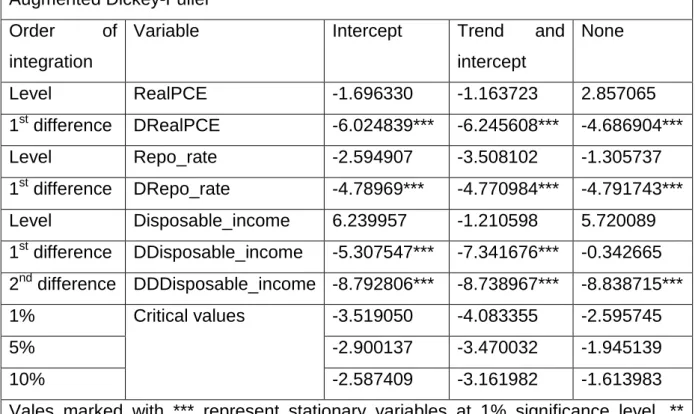
Table 4.1: Stationarity results of the Augmented Dickey-Fuller test
Augmented Dickey-Fuller Order of
integration
Variable Intercept Trend and intercept None Level RealPCE -1.696330 -1.163723 2.857065 1st difference DRealPCE -6.024839*** -6.245608*** -4.686904*** Level Repo_rate -2.594907 -3.508102 -1.305737 1st difference DRepo_rate -4.78969*** -4.770984*** -4.791743*** Level Disposable_income 6.239957 -1.210598 5.720089 1st difference DDisposable_income -5.307547*** -7.341676*** -0.342665 2nd difference DDDisposable_income -8.792806*** -8.738967*** -8.838715*** 1% Critical values -3.519050 -4.083355 -2.595745 5% -2.900137 -3.470032 -1.945139 10% -2.587409 -3.161982 -1.613983
Vales marked with *** represent stationary variables at 1% significance level, ** represents stationarity at 5% significance level and * represents stationarity at 10% significance level.
Table 4.1 shows the Augmented Dickey-Fuller (ADF) results. The test has a null hypothesis of unit root. When the results show that the calculated t-value is greater than the critical value, the null hypothesis is rejected, and the conclusion is that there is no unit root, or the series are stationary. The ADF tests the variables at intercepts, trend and intercepts and at no trend and intercept. When looking at the intercept, all the variables are non-stationary in levels at all listed levels of significance. All the variables, at first difference, D(I), were stationary at 1% significance level and the null hypothesis of non-stationarity was rejected.
27
4.2.2 Heteroscedasticity results
The results for heteroscedasticity tested using the Koenker Bessett test (KB) are shown on table 4.2 below. The results show the value of the F statistic for the Household final consumption expenditure model is F(1,67) = 0.0012. The critical value of the test at 5% level of significance is approximately 4 (3.84). The study then fails to reject the null hypothesis concluding no evidence of heteroscedasticity.
Table 4.2 Heteroscedasticity results of the Koenker Basset test (KB)
Koenker-Bassett test results
Variable Coefficient Standard Error T-Stat P-value
Constant 0.519 0.117 4.427 0.000 𝑌̂2 -0.001 0.026 -0.035 0.973 Regression F(1,67) 0.0012 Durbin-Watson Statistic 1.8243 Significance Level of F 0.973 4.2.3 Autocorrelation results
The results for autocorrelation are given in figure 4.1 below. At lag 1, the correlation is shown as being around 0.9 as the data is correlated to itself. There is then negative correlation from lag 11 to 16.
28
Figure 4.1: Autocorrelation function (ACF)
4.3 Does repo rate impact consumption spending in the short run?
The first method of the study runs impulse responses in order to assess the dynamic path followed by consumption after an unexpected increase in the repo rate. To do so, VAR models are used. The models are estimated using the Choleski ordering. The number of lags used in the estimation process is selected using the Akaike information criterion as well as the Schwarz Bayesian criterion or Bayesian information criterion (BIC). The models are estimated using two lags. Figure 4.2 shows the impulse responses of growth in real consumption expenditure to positive repo rate changes.
29
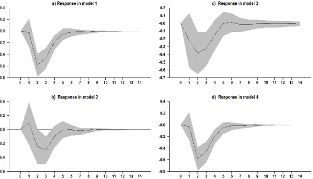
Figure 4.2: Responses of growth in real consumption expenditure to positive repo rate changes
The results in figure 4.2 above represent four different models. Model 1 reflects the impulse response of real Household final consumption expenditure to an increase in the repo rate. The results show that an increase of 100 basis points in the repo rate leads to a decrease in Household final consumption expenditure. The effect appears to be temporary as it lasts for up to 6 quarters. The second model adds disposable income in the model in order to test for robustness. The results still show that an increase in the repo rate leads to a decrease in Household final consumption expenditure. Model 3 adds two extra variables to model 2, household debt and household assets to further test for robustness. The results still show a negative correlation that lasts for 5 quarters. The fourth model seeks to investigate the importance of ordering in the model. Household final consumption expenditure is put first followed by the repo rate, opposite of model 1. The results are exactly similar to those obtained in model 1 and this indicates that ordering does not matter in the model
30
4.4 Cointegration test and the long run relationship
The stationarity test indicates the variables are integrated of the same order, which enables me to proceed and determine whether there exists a long-run relationship amongst them. For the purposes of this study cointegration examines the long-run relationship amongst the household final consumption expenditure, repo rate and household disposable income. The Household final consumption expenditure is deflated by consumer price index. The household debt and household assets were used in to test robustness in the analysis of short run effects of repo rate.
The study uses the Johansen (1995) cointegration approach to test for cointegration. The results of the cointegration test are shown in table 4.3 below. The two-test used in the Johansen cointegration approach are the trace and maximum eigenvalue.
Table 4.3: Cointegration results
Sample: 1999Q1 2018Q2 Included observations: 73
Series: LRPCE LDISP REPO_RATE Lags interval: 1 to 4 Selected (0.05 level*) Number of Cointegrating Relations by Model
Data Trend: None None Linear Linear Quadratic Test Type No Intercept Intercept Intercept Intercept Intercept
No Trend No Trend No Trend Trend Trend
Trace 1 1 1 1 1
Max-Eig 1 1 1 1 1
*Critical values based on MacKinnon-Haug-Michelis (1999)
Table 4.3 shows the summarised results of the trace and the maximum Eigen value tests. The null hypothesis of no co-integrating vectors is rejected since both the trace and the maximum Eigen tests both specified one co-integrating relationship at 5% significance level. This suggests there is one significant long-run relationship between the given variables.
31
4.5 Results of the estimated long run equation
The detection of a cointegration equation in the previous section means that a long run relationship can be estimated. The variables are estimated in logarithmic format except the repo rate which is expressed in per cent. The long run equation is estimated using ordinary least squares (OLS) and includes a dummy which equals to one during recession in 2009Q1-Q3 and 2018Q1-Q2 and zero otherwise. Results clearly show that long run cointegration relationships exist among the variables and are presented in Table 4.4 below.
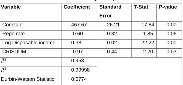
Table 4.4: Results of the estimated long run equation
Variable Coefficient Standard
Error
T-Stat P-value
Constant 467.67 26.21 17.84 0.00
Repo rate -0.60 0.32 -1.85 0.06
Log Disposable income 0.38 0.02 22.22 0.00
CRISDUM -0.97 0.44 -2.20 0.03
𝑅̅2 0.953
𝑅2 0.99998
Durbin-Watson Statistic 0.0774
In table 4.4, the dependant variable is household final consumption expenditure. The results of equation 3.5 indicate that 99.99% of variations in household final consumption expenditure are explained by changes in the repo rate, disposable income and whether or not there is a recession. All the variables are significant at least at 10% significance level.
The impact of the repo rate on household final consumption expenditure is negative and significant at 10%. The coefficient of -0.60 for the repo rate indicates that, all things being equal, a 1 percent increase in the repo rate reduces Household final consumption expenditure by approximately 0.6%. This means that the repo rate exerts a negative influence on household consumption. This negative relationship is consistent with economic theory and is in agreement with the work of Kapor and
32
Ravi (2009), Ghana et al. (2014) and contradicts with the work of Vengel (2015) who found a positive correlation between interest rates and household consumption. This implies that when monetary policymakers raise the policy rate, South African households cut off their consumption.
Disposable income has a significant and positive impact on consumption and the coefficient indicates that, all things held constant, a 1 per cent increase in disposable income raises Household final consumption expenditure by approximately 0.38%. This positive relationship between disposable income and Household final consumption expenditure is consistent with Keynes’ absolute income theory which states that consumption grows with increasing income (Keynes, 1936) and is also consistent with the empirical work of Nicklaus (2015). The regression results suggest that as household disposable income increases, in turn households increase their final consumption in the long run.
The coefficient of -0.97 in the crisis dummy (CRISDUM) suggests that the recession reduced household expenditure by approximately 1%. These results are consistent with economic expectations and conform to the study’s predictions.
4.6 Evidence of sign asymmetry test
Following the estimation of the long run relationship results I then proceed to determine the prevalence of the sign asymmetry by estimating short run equation (3.6) mentioned in chapter 3.
In Table 4.5, a positive repo rate change (Δ Positive repo rate) lowers consumption expenditure significantly at 5% significance level. The results show that a 1% increase in the repo rate hampers Household final consumption expenditure by 0.8%. In contrast, negative repo rate changes raise consumption significantly. The negative repo rate changes variable (Δ Negative repo rate) has a coefficient of 0.56 implying that a 1% decrease in the repo rate raises Household final consumption expenditure by approximately 0.56%. The sign of the coefficient of disposable income is still similar to the one obtained from the long run relationship estimation results.
33
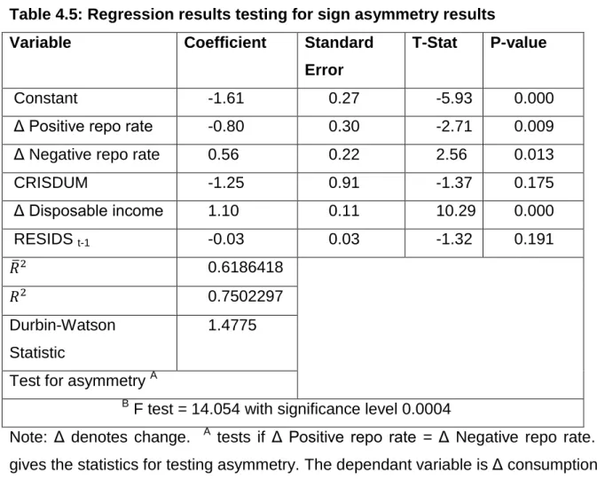
Table 4.5: Regression results testing for sign asymmetry results
Variable Coefficient Standard
Error
T-Stat P-value
Constant -1.61 0.27 -5.93 0.000
Δ Positive repo rate -0.80 0.30 -2.71 0.009 Δ Negative repo rate 0.56 0.22 2.56 0.013
CRISDUM -1.25 0.91 -1.37 0.175 Δ Disposable income 1.10 0.11 10.29 0.000 RESIDS t-1 -0.03 0.03 -1.32 0.191 𝑅̅2 0.6186418 𝑅2 0.7502297 Durbin-Watson Statistic 1.4775
Test for asymmetry A
B F test = 14.054 with significance level 0.0004
Note: Δ denotes change. A tests if Δ Positive repo rate = Δ Negative repo rate. B gives the statistics for testing asymmetry. The dependant variable is Δ consumption The results show that a 1% increase in household disposable income raises Household final consumption expenditure by approximately 1.1%, all things held constant. Disposable income is significant at 5% significance level. The results also show a negative coefficient for the crisis dummy. This indicates that in the event of a recession, Household final consumption expenditure decreases by approximately 1.3%. The results are consistent with economic theory and fulfil the expectations of the study.
The study assesses the potential asymmetric effects of interest rate (repo rate) changes on household consumption. The results for sign asymmetry are presented in Table 4.5. The sign asymmetry is tested by 𝛽4 ≠ 𝛽6 in equation 3.7. The results
show different signs and magnitudes for the coefficients of positive and negative repo rate changes and the asymmetry test as indicated by A in table 4.5 show that positive and negative repo rate changes are statistically different and significant at 5% significance level. This implies the existence of sign asymmetry. The coefficient of positive repo rate (Δ Positive repo rate) changes, 𝛽4, has the value -0.8 which is
34
different from that of negative repo rate (Δ Negative repo rate) changes, 𝛽6, whose
value is 0.56. Both coefficients are statistically significant at 5% significant level. These results prove the existence of sign asymmetry and the null hypothesis of asymmetry where 𝛽4 ≠ 𝛽6 is not rejected.
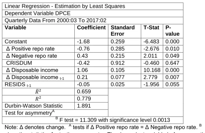
4.7 Robustness test results
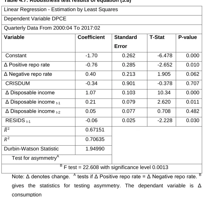
This section tests the robustness of the findings that were obtained in the previous section. Robustness is tested by including the role of consumption smoothing in equations (3.7) and (3.8). Consumption smoothing is captured through the addition of the first and second lags of consumption as determinants of current consumption. This is motivated by the Franco Modigliani’s life-cycle hypothesis which implies that individuals do not usually save up a lot in one period to spend furiously in the next period and aim to keep their consumption levels smooth.
In Tables 4.6 and 4.7, the lagged consumption has positive effect on current consumption, which indicates the prevalence of consumption smoothing. The results show that consumption in the previous period increases current consumption by approximately 0.21% while consumption in the previous two periods raises consumption by about 0.05%. Thus, consumption today is influenced by consumption in the previous period quarter.
The signs of the coefficients of the other variables in the models still conform to the results obtained from the sign asymmetry test although the magnitudes have changed. The results based on the short run equations are robust to different estimations and inclusion of additional variables.
35
Table 4.6: Robustness test results of equation (3.7)
Linear Regression - Estimation by Least Squares Dependent Variable DPCE
Quarterly Data From 2000:03 To 2017:02
Variable Coefficient Standard
Error
T-Stat P-value
Constant -1.68 0.259 -6.483 0.000 Δ Positive repo rate -0.76 0.285 -2.676 0.010 Δ Negative repo rate 0.43 0.215 2.011 0.049 CRISDUM -0.42 0.912 -0.460 0.647 Δ Disposable income 1.06 0.105 10.168 0.000 Δ Disposable income t-1 0.21 0.077 2.779 0.007 RESIDS t-1 -0.05 0.025 -1.956 0.055 𝑅̅2 0.659 𝑅2 0.779 Durbin-Watson Statistic 1.891 Test for asymmetryA
B F test = 11.309 with significance level 0.0013
Note: Δ denotes change. A tests if Δ Positive repo rate = Δ Negative repo rate. B
36
Table 4.7: Robustness test results of equation (3.8)
Linear Regression - Estimation by Least Squares Dependent Variable DPCE
Quarterly Data From 2000:04 To 2017:02
Variable Coefficient Standard
Error
T-Stat P-value
Constant -1.70 0.262 -6.478 0.000
Δ Positive repo rate -0.76 0.285 -2.652 0.010 Δ Negative repo rate 0.40 0.213 1.905 0.062
CRISDUM -0.34 0.901 -0.378 0.707 Δ Disposable income 1.07 0.103 10.34 0.000 Δ Disposable income t-1 0.21 0.079 2.620 0.011 Δ Disposable income t-2 0.05 0.077 0.708 0.482 RESIDS t-1 -0.06 0.025 -2.228 0.030 𝑅̅2 0.67151 𝑅2 0.70635 Durbin-Watson Statistic 1.94990 Test for asymmetryA
B F test = 22.608 with significance level 0.0013
Note: Δ denotes change. A tests if Δ Positive repo rate = Δ Negative repo rate. B
gives the statistics for testing asymmetry. The dependant variable is Δ consumption
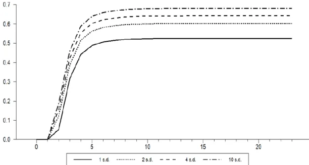
4.8 Evidence of Size asymmetry
Using the Killian and Vigfussion (2011) approach to test for size asymmetry, the size asymmetric test is conducted using equation (3.9) from chapter three, with the first equation similar to the standard linear VAR in 𝑅𝑡 and 𝐶𝑡, but the second equation
includes both 𝑅𝑡 and 𝑅𝑡+. 𝑅𝑡+ in the second part of equation (3.9) is replaced by 𝑅𝑡− such that both the effects of positive and negative repo rate changes on Household final consumption expenditure are captured in the model in order to test size asymmetry.
37
The size asymmetry is tested separately for both positive and negative repo rate changes. Figures 4.3 and 4.4 below show the results of size asymmetry obtained by equation (9) and 𝑅𝑡+ is replaced by 𝑅𝑡− in order to determine the size asymmetry related to negative interest rate changes.
Figure 4.3: Size asymmetry results for repo rate loosening shocks
Figure 4.3 shows the magnitude of the repo rate changes represented by the standard deviations (s.d). A 1 standard deviation indicates a lower decrease in repo rate and 10 standard deviations representing a higher decrease in the repo rate. Hence Figure 4.3 shows the impulse responses based on the size of repo rate reduction shocks. One standard deviation is lower than 2, 4 and 10 standard deviations. This is to say that a decrease of 25 basis points in the repo rate raises Household final consumption expenditure much lower that a decrease of 100 basis points. This proves the existence of sign asymmetry as the different repo rate size contractions have different magnitude effects on Household final consumption expenditure although the signs are the same for the same directional change.
38
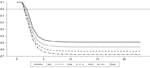
Figure 4.4: Size asymmetry results for repo rate tightening shocks
The results in Figure 4.4 show the presence of size asymmetry during monetary policy tightening. The results indicate that a lower increase in the repo rate leads to a lower decrease in household consumption, whereas a higher increase in the repo rate causes a higher decrease in household consumption. This implies that an increase of 25 basis points in the repo rate reduces Household final consumption expenditure much lower that an increase of 100 basis points. This also proves the existence of sign asymmetry as the different repo rate size increases have different magnitude effects on Household final consumption expenditure although the signs are the same for the same directional change (contraction).
39
CHAPTER FIVE
FINDINGS, RECOMMENDATIONS AND CONCLUSION
5.1 Introduction
This chapter concludes the whole study. It gives a summary of the major findings obtained from the study as well as their policy implications. It further provides recommendations based on the findings of the study.
5.2 Summary of findings
Having applied both economic and econometric tools to thoroughly analyse the asymmetric effects of repo rate changes on household final consumption expenditure in South Africa, the following summarised findings were obtained from the study.
It was found in the study that there exists a negative relationship between a positive repo rate changes and household final consumption in the long run. The long run relationship results revealed that, a percentage increase in the repo rate leads to reduction of approximately 0.60% in household final consumption expenditure. The results obtained in the sign asymmetry test results (short run) showed that a 1 percent increase in the repo rate leads to a contraction of approximately 0.80% in household final consumption expenditure.
The study further found that there exists a positive relationship between negative repo rate changes and household consumption. The sign asymmetry test results revealed that a 1% reduction in the repo rate stimulates Household final consumption expenditure by approximately 0.56%. The study found the existence of sign asymmetry in repo rate changes on household final consumption expenditure, with the two beta coefficients for both negative and positive repo rate changes unequal and significant at 5% significance level.
The study also revealed that there exists a positive relationship between Household final consumption expenditure and disposable income in both the short and long run. A 1% increase in household disposable income induces Household final consumption expenditure by approximately 0.38% in the long run. In the short run, a
40
1% increase in disposable income induces Household final consumption expenditure by 1.1% in the short run. After having tested for robustness in the sign asymmetry test, the results revealed that past consumption patterns have a positive effect on current consumption. Furthermore, the study found that in the event of a recession, Household final consumption expenditure declines by approximately 0.97% in the long run. The negative relationship still prevails in the short run, with Household final consumption expenditure declining by 1.25% in the event of a recession.
The study also proved the existence of size asymmetry in repo rate changes on household consumption. The results indicate that a bigger change in the repo rate leads to a bigger change in household consumption. An increase of 0.25% in the repo rate will lead to a lesser contraction in Household final consumption expenditure that a 1% increase. Furthermore, the results indicate that a 1% cut in the repo rate will induce Household final consumption expenditure more than a 0.25% cut. This indicates that the bigger the change, the larger the response, confirming that there is sign asymmetry on the effects of repo rate changes on household consumption.
5.3 Policy implications and recommendations
The findings outlined in the previous section have some policy implications. The findings in the previous chapter have shed some light on a major policy instrument that has a significant effect on household consumption. In view of this, recommendations have been to help policy makers induce or reduce Household final consumption expenditure depending on the South African economic state.
Positive repo rate changes have a negative impact on Household final consumption expenditure both in the long run and short run. The implication is that, increasing the repo rate with the aim of inducing household savings will be effective in the long run and short run but the effect is not permanent. Also, the higher the interest rate increase, the more reduction in household’s consumption. This implies that if policy makers want to cut household consumption, then there is need for a higher increase in the repo rate.
Negative repo rate changes have a positive impact on Household final consumption expenditure both in the long run and short run. The implication is that, in an attempt to induce Household final consumption expenditure in order to stimulate economic