Working Paper Series
Exchange Rate Pressure in Angola
Francesco Franco
Nova School of Business and Economics, Universidade Nova de Lisboa
Júlio António Rocha Delgado
INOVE Research
–
Investigação & Desenvolvimento
Suzana Camacho Monteiro
BNA
–
Departamento de Estudos Económicos
Pedro Castro e Silva
BNA
–
Departamento de Estudos Económicos
ISSN 2183-0843
NOVAFRICA Working Paper Series
Any opinions expressed here are those of the author(s) and not those of NOVAFRICA.
Research published in this series may include views on policy, but the center itself takes
no institutional policy positions.
NOVAFRICA is a knowledge center created by the Nova School of Business and
Economics of the Nova University of Lisbon. Its mission is to produce distinctive
expertise on business and economic development in Africa. A particular focus is on
Portuguese-speaking Africa, i.e., Angola, Cape Verde, Guinea-Bissau, Mozambique,
and Sao Tome and Principe. The Center aims to produce knowledge and disseminate it
through research projects, publications, policy advice, seminars, conferences and other
events.
NOVAFRICA Working Papers often represent preliminary work and are circulated to
encourage discussion. Citation of such a paper should account for its provisional
Exchange rate pressure in Angola
Francesco Franco, Júlio António Rocha Delgado, Suzana Camacho Monteiro and Pedro Castro e Silva
May 2014
Abstract
The objective of this work is to develop an operational tool to analyze exchange rate pressure in the context of Angola. The Angolan economy exhibits a number of relevant characteristics: a closed financial account, a partially controlled current account, a highly dollarized economy and exports (oil) price determined in World markets. These features have a direct effect on the demand of foreign currency and motivate their inclusion in the specification of a model for Angola. The model provides the rational for a measure of an exchange market rate pressure (EMP) index that contains exports changes, imports changes, the foreign interest rate and inflation and the change in foreign reserves corrected for a measure dollarization. The empirical performance new measure is comparable (slightly better) to the performance of the EMP indexes obtained in Eichengreen Rose and Wyplosz (1994) and Klassen and Jager (2011).1
Introduction
The objective of this work is to develop an operational tool to analyze exchange rate pressure in the context of Angola. Exchange rate pressure is a broad concept that can encompass every deviation of the actual exchange rate from a latent equilibrium exchange rate. Deviations can originate from macroeconomic forces, and are typically labeled misalignments in the international macro literature, or from financial forces, which because of their higher frequency relative to macro forces, (probably) gave rise to the label of pressure. In this work we will use pressure for both types of deviations. By taking this view we can trace back interest in exchange rate pressure and misalignment with the active management of the exchange rate by the monetary authorities. Formal high frequency empirical measures of exchange rate pressure are more recent and started in the late 1970’s. The existing literature on this later subject can be divided into two branches.
1
The first branch derives a measure of exchange rate pressure from a model of exchange rate determination. Girton and Roper (1977) are maybe the first example of this approach. More recent examples are Weymark (1997). Their objective is to measure the excess demand for a currency by deriving the gap between the observed exchange rate and a notional exchange rate that would prevail in a pure floating regime conditional on current monetary policy. The vast literature on currency crisis that started with Krugman (1979), Flood and Garber (1984) and then continued with Obstfeld (1994) is closely related. Indeed, most models of speculative attacks derive a “shadow” exchange rate, usually defined as the implicit floating exchange rate that would prevail once reserves are exhausted. While the shadow exchange rate and the notional exchange rate just defined are different, the approach is conceptually similar and both require estimating the structural parameters of the model used in the analysis.
The second strand follows the observation from Meese and Rogoff (1983) that models linking variables like reserve flows and interest rates to the exchange rate appear to be inadequate. A particular set of weights and fundamentals is only as defensible as the theoretical model used to generate it. Eichengreen Rose and Wyplosz (1994) propose an index of exchange rate market pressure model-free. In practice they construct an index using a linear combination of the same variables used in most models but consider a number of different weighting schemes induced by the data. Klassen and Jager (2011) follow a similar approach. First they specify a standard monetary model with an endogenous monetary policy response in the form of Taylor rule and obtain the insight that the policy interest rate should enter in levels and not in differences, then derive a model-free weighting scheme to construct the exchange market pressure measure that now contains the interest rate in level.
Conceptually going back and forth between a model based approach and a data induced analysis is the correct approach. In principle we would like to identify the variables involved in the exchange rate pressure from a sufficiently general class of models and subsequently bring it to the data. However for the exercise to be meaningful, the class of models should be appropriated to describe the economy under investigation. The Angolan economy is characterized by several features that require particular attention in order to infer the correct variables that should be used to measure exchange rate pressure.
The determination of the exchange rate and the derivation of a pressure
measure
The level of the exchange rate has proven to be a difficult variable to determine. This difficulty is an issue given the influence of the exchange rate in an integrated World economy and must be considered when evaluating measures of deviations from notional or equilibrium exchange rates. To illustrate the basic insights we will proceed by illustrating a simple benchmark example.
If a currency was only traded spot in a centralized exchange, its relative price would be simply determined by demand and supply. Trades involving a currency can occur because of current account transactions (trade in goods, services, income payments, transfers) or financial account transactions (FDI, Portfolio, Trade credits, Banks deposits, Loans). Let CAt = P CAt−N CAt be the current account which is equal to the difference between
positive flows and negative flows. Let KAt = ∆F DAt−∆DF At the capital-financial account which is equal to
the difference between the change in foreign domestic assets and domestic foreign assets. The equilibrium exchange rateEe
t is such that
KAt(Eet, zKA,t) +CAt(Ete, zCA,t) = 0,
where thezCA, zKAare all the other variables affecting the current and financial accounts. In a World with perfect
markets, a pure floating exchange rate would always equal its equilibrium value. The actual exchange rateEt can
differ from the equilibrium exchange rateEe
t because of imperfections, frictions and defects of the financial markets
and/or non-optimal management of the exchange rate by the national monetary authority. The exchange market rate pressure is therefore:
EM Pt=Et−Ete.
The difficulties begin with the specification of a model. The majority of the literature on EMP uses some variant of a macroeconomic monetary model. In the spirit of Girton and Roper (1977), consider a simple log-linear model with a standard money demand:
md
t −pt=φyt−ηit,
wheremd is the demand of money,pis the price level,yis the level of income andiis the relevant short term rate.
All variables are in natural logarithms except the interest rate. φ and η are the respective (semi-)elasticities and are considered structural parameters of the economy. The money supply is
mst=rt+dt,
wherertare foreign reserves expressed in domestic currency anddtis domestic credit. Both are expressed in natural
rate, denotedet, through a purchasing power parity (PPP) condition
pt=p∗t +et.
Starred variables denote foreign variables. Solving for the money market equilibrium, using PPP and a symmetric model for foreign imply:
et+ (it−i∗t)−(rt−rt∗) = (dt−d∗t)−φ(yt−yt∗) + (1 +η)(it−i∗t).
The left hand side is an index of exchange rate pressure: if domestic reserves of foreign exchange decline or interest rates rise or the exchange rate depreciates, pressure increases. Sometimes the monetary model is augmented with an uncovered interest parity, see for example Weymark (1997), which changes the exchange rate determination to an asset model. Consider the uncovered interest parity
it=i∗t+Et[et+1]−et+ψt
where ψt is a risk premium and Et is the mathematical expectation operator. Solving forward, the exchange
rate is determined by:
et= 1 1 +η
∞
X
s=t
η
1 +η
s−t
Et[rs+ds−φys+ηi∗s+ηψs−p∗s].
Modeling or assuming the path of the variables in the right hand side we can solve for the equilibrium exchange rate and construct a measure of of EMP by taking deviations of the actual exchange rate from the model derived exchange rate. One problem with this approach is that the data are not very kind to this monetary model (outside maybe hyper-inflationary environment). A further complication arises because of the necessity of estimating struc-tural parameters. A simple solution is to bypass the estimation of the strucstruc-tural parameters and use a more reduced form approach like in Eichengreen Rose and Wyplosz (1994) intuitive, although arbitrary, proposal to weight the components of the index implied by the monetary model so that their conditional volatilities are equal.
Angola overview
as well is subject to controls2
. There are other aspects of the Angola economy, such as the fact that exports are overwhelmingly oil and gas whose price can be taken a exogenous or that the economy is heavily dollarized that deserve special attention in the specification of a model of exchange rate determination. This sub-section presents rapidly some stylized facts to motivate the modeling assumptions of the next section.
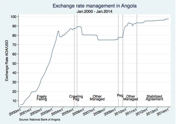
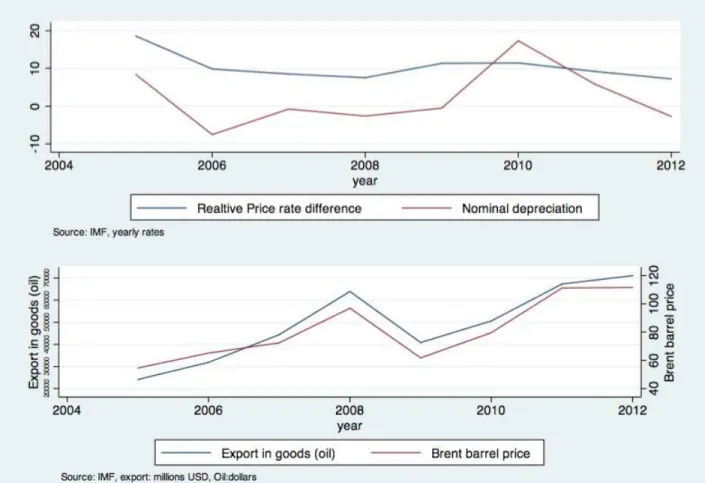
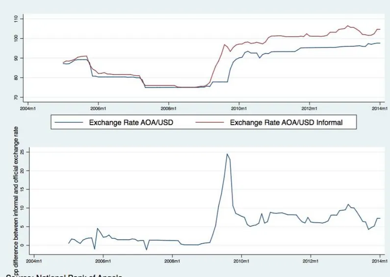
Figure 1 shows the last fifteen years of exchange rate regimes in Angola that started de facto an successful exchange rate management in early 2005. Figure 2 shows the components of the Financial account and the current account from 2005 to 2012. The figure shows the tight management of the financial account through foreign reserve management. Notice that during the last three years of the sample current account surpluses have increasingly financed direct investment. Figure 3 shows the nominal annual effective depreciation of the Angolan currency and the annual effective price differential between the Angolan CPI and its trading partners. Except for the global financial crisis that corresponded to a relatively large 17 percent depreciation of the Angolan currency, the inflation differential appears to play the more important role in the dynamics of the real exchange rate. It is worth noting that the inflation differential was not affected by the depreciation during the crisis. This observation suggests a degree of control of the domestic inflation by the central bank relatively independent of the exchange rate management. The second panel of Figure 3 shows the level of exports in goods together with the price of a barrel of oil in the World market. Given that virtually (98%) of goods exports are oil and gas and that domestic energy production has been peaking in 2008 and then remained flat, changes in the level of export in goods are mostly driven by price changes and are exogenous to Angola. Figure 4 shows the level of foreign reserves, the money supply (M2), the amount of foreign currency deposits and the money multiplier (the ratio of M2 to reserve money). Until 2009 foreign reserves were fully backing the existing supply of M2. Since 2009 M2 has become larger than the Foreign reserves but their ratio has been kept sufficiently stable. A more detailed analysis of this symptom of dollarization requires a more complete set of data. The IMF second post program report provides some information on the amount of foreign currency deposits which approximately still stand at 50% of M2 while the amount of foreign currency credit to the private sector stands at 63.8% in 2009. The important role of the dollar as a medium of exchange and store of value in Angola creates an important source of trade in dollars against kwanzaas that can impact on the exchange rate. Informal currency trade within Angola is also an important source of pressure on the exchange rate. Figure 5 shows the evolution of the informal and official exchange rate against the dollar and the percentage difference between the informal and the official exchange rate. At the peak of the crisis, the informal exchange rate was trading at a 25% lower value than the official rate. Since then the lower informal value appears to have fluctuated within a 5% to 10% corridor. Notice that the post-crisis corridor is sensibly higher (larger discount) than the one prevailing before the crisis which oscillated between -1% and 5%. The higher corridor coincides with the less than complete backing of money by Foreign reserves.
A synthetic narrative that comes from this short description is that oil exports, mostly determined by the world
2Today, membership to the IMF requires full liberalization of the current account, and national discretion for what regards the degree
oil price are the primary source of foreign currency. The shock of the global crisis in 2009 decreased oil price from an average of 100 us dollars in 2008 to an average of 60 us dollars in 2009. The same year, Angola experienced the only episode of current account deficit in the sample which was followed by a sharp depreciation. Angola is also a highly dollarized economy. This characteristic can play an important role in the exchange rate determination by generating pressures originating from domestic credit and financial shocks unknown in countries with a single national domestic tender.
The next section presents a simple model for Angola. The scope is to start the construction of a relevant macroeconomic model for Angola whose features will be incorporated progressively in a series of future works. This is the first of these works and is necessarily incomplete, for example it does incorporate the dollarization of the economy in an extremely reduced form. It also lacks other aspects of the Angolan economy which are likely to be important. Again, in this work, the scope of the model is to identify the relevant variables to be incorporated in the empirical analysis. The non technically oriented reader can skip the section and directly jump to the empirical part.
A benchmark model for Angola
The observations of the previous section motivate a specification of a benchmark model for Angola that features the following key simplifying assumptions:
• the Central Bank (CB) manages the exchange rate through foreign exchange reserves operations, • the CB controls the short term interest rate to control domestic inflation,
• exports (oil) are exogenous.
The core of the model is a small open economy (SOE) new Keynesian model. Furthermore the benchmark model features the following simplifying technical assumptions (non-crucial):
• unit elasticity of substitution between nontradables and imports • log utility in consumption
• constant return to scale in production of non tradable.
We present for simplicity a log-linearized version of the model (See appendix for the non-linear model). Aggregate consumptionctis a composite index of non-tradable goodscN,t, produced domestically, and imported goodscM,t:
ct=ωcN,t+ (1−ω)cM,t
where ω is the share of nontradables. Demand for each good is a function of aggregate expenditure and its relative price
cN,t=ct−qN,t,
cM,t=ct−qM,t,
where qN,t is the price index for nontradables deflated by the CPI andqM,tis the price of imports deflated by
the CPI pt. The latter depends on the nominal exchange rateet and the foreign price of importspF,t deflated by
CPI
qM,t=et+ (pF,t−pt).
Aggregate expenditure depends on the term structure of real interest rates relevant for consumption decisions (Euler equation)
ct=Etct+1−Et(iD,t−πt+1−ρ)
whereiD,tis the one period nominal interest rate (policy rate) andπtis the rate of CPI inflation. ρ=−log(β)and
β is the time discount factor. The labor supply comes from household first order condition
(wt−pt) =ct+φnt.
The non-tradable sector outputyN,t is produced with a constant return to scale in labor inputnt
yN,t=at+nt
whereatis labor productivity. Non-tradable producers are price setters subject to nominal price rigidity (a la Calvo
with parameterθ) which results in a standard new Keynesian Phillips curve
πN,t=βE{πN,t+1}+λmct
mct= (wt−pt)−qN,t−at.
The non-tradable clearing market condition implies
yN,t=cN,t.
Importers (price setters or not) face flexible prices so that imported goods inflation is
πM,t= ∆et+πF,t.
CPI inflation is
πt=ωπN,t+ (1−ω)πM,t.
The national budget constraint is
ζft=ζL(ft−1+iF,t−1−∆et−πF,t) +ζOyO,t−CMcM,t
where ft is foreign exchange reserves (in foreign goods). yO,t is the exogenous real exports of oil, iF,t is the
exogenous foreign interest rate on foreign reserves andπF,tthe foreign inflation rate3.
Finally policy consists in choosing a path fore¯tby managing foreign reserves and setting the domestic interest
rate iD,t. From a simplified Central Bank balance sheet, define χt =ln
EtFt
Mt µt
where M is money and µ the money multiplier. Levels inχtsignal the capacity of the Central Bank to face domestic demand of foreign currency.
Changes inχtcan be seen as an index of sterilization(∆χt= 0, implies full sterilization).
Empirical Analysis
The above model provides the rational for a measure of an exchange rate pressure index that contains exports changes, imports changes, the foreign interest rate and inflation and the change in foreign reserves corrected by our measure χt. Following Eichengreen Rose and Wyplosz (1994) the weights of the components of the index are
set so that their conditional volatilities are equal. A second measure is obtained by selecting a subset of the above variables by eliminating those that are statistically insignificant in predicting one month ahead a devaluation of 2 percent (annual rate). The 2 percent threshold corresponds to the band defined by the monetary authority within the exchange rate is managed. Finally the two measures of EMP are compared with the EMP indexes obtained in Eichengreen Rose and Wyplosz (1994) and Klassen and Jager (2011). All the data used in the analysis are presented
3
ζ=F+ρF(F)QFM
, ζL=(1+∆QiMF)ΠF, ζO=
POYO
PF ,where capital letters without time subscript indicate steady state values andρF
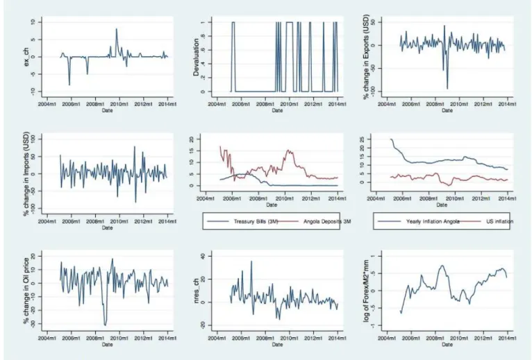
in Figure 6:
• the exchange rate monthly depreciation rate∆et,
• a binary index of devaluation that takes the value of 1 if the exchange rate depreciates more than 2% on an annual basis,
• the percentage monthly rate of change in exports denominated in dollars∆xt,
• the percentage monthly rate of change in imports denominated in dollars∆mt,
• the US 3-month T-billiF,t,
• the Angola 3 month deposit rateiD,t,
• the US annual inflation rate πF,t,
• the Angola annual inflation rateπA,t,
• the percentage change in oil prices (Brent),
• the monthly percentage change in foreign reserves ft,
• and the index χt which is the ratio of Foreign reserves denominated in domestic currency to the money in
circulation (M2) times the money multiplier (demeaned).
The sample starts in 2005. The EMP measure that follows from the model of the previous section is:
EM Ptheory = ∆et+α∆f∆ft+αiFiF,t−1−απFπF,t−α∆x∆xt+α∆m∆mt−αχχt
where the αy = stdevstdev(∆(yett)). The second suggested measure of EMP is derived by keeping in the index only the
variables suggested by the model that significantly predict one month ahead a devaluation of more than 2% percent at an annual rate. Table 1 presents the probit regressions where the dependent variable is devaluation and the explanatory variables are the one month lagged variables.
The EMP measure that follows the model and the statistical approach is:
EM Pempirical= ∆et+αiFiF,t−1−α∆x∆xt−αχχt.
For comparison we report the index of Eichengreen Rose and Wyplosz (1994) based on the arbitrary same weighting scheme and on monetary model:
and the Klassen and Jager (2011) index based on a modified monetary model that endogenizes monetary policy with an interest rate rule, define the notional exchange rate the exchange rate that would have prevailed without intervention and use the same weighting scheme:
EM PKJ = ∆et−αf mf mt+α(iF−iD)(iF,t−iD,t),
wheref mt=∆FMttEt−1
−1
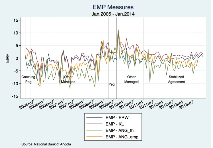
.Figure 7 shows the four different measures. Finally, Table 2 compares the predictive power
of the four measures in anticipating a devaluation by one month regressing the variable devaluation on the four lagged EMP indexes. For each index three models are estimated: OLS, Probit and Logit. The reason for the probit and logit models is that the dependent variable is a discrete variable that takes the value 1 in the event of the depreciation greater than 2 percent (yearly rate) and 0 in the event of no depreciation (or smaller than 2 percent). Formally, letyt∈[0,1], t= 1, ..., T. Letθt=P r[yt= 1], which is a function on the exchange market rate pressure
via
h(θt) =yt∗=βEM Pit−1+uit,
whereiindexes the different EMP measure andyt∗ is the depreciation rate. Therefore
yt=
0 , y∗t <2% 1 , y∗t ≥2%
For probit, uit is N(0,1), while for logit uit is drawn from a logistic distribution, also normalized to have unit
variance. The log-likelihood function is easy to construct in the case of independent4
yt. For comparison the
OLS results are reported as well. The estimates from the three models tell a consistent story. The signs of the coefficients are the same across the models, and the exchange market pressure measures are statistically significant in each model. The three models are estimated with robust standard errors. The four EMP measures have predictive power. Overall the ranking isEM Pempirical≻EM PKJ ≻EM Ptheory≻EM PERW. EM Ptheoryhas a performance
comparable (slightly better) with EM PERW while EM Pempirical has a performance comparable (slightly better)
withEM PKJ. Consider the results for the probit model usingEM Pempirical as an explanatory variable:
yt∗=−.7256997 + 0.312683EM Pit−1,
4Absence of independence across time of the dependent variables is potentially problematic and can substantially complicate the
estimation. The simplest test is to assume a transitional model in which correlation among the discrete responses arises because past responses explicitly influence the present outcome. Past realizations of the discrete response help determine the current response, and so enter the model as additional predictor variables. Assuming a Markov chain to form the basis of a transitional model, Diggle, Liang and Zeger (1994, 135) show the model:
h(θt) =β0EM Pit−1+αEM Pit−1yt−1+uit,
Tests of the null hypothesisα= 0tap whether the effects of EMP are constant irrespective of the previous state of the binary process.
where both the constant and the coefficient are highly significant. The interpretation is that in the monthly sample (2005-2013) ifEM Pemprical= 0then the probability of a devaluation greater than 2% is equal to 0.23 (Φ(−0.72),
where Φis the cdf of aN(0,1)) while ifEM Pempirical is equal to the sample average (-1.203529 ) the probability
becomes 0.13 (Φ(−0.72 + 0.31×(−1.22))). Compare these results with the logit model:
y∗t =−1.256036 + 0.5484EM Pit−1.
WhenEM Pemprical= 0then the probability of a devaluation greater than 2% is equal to 0.22 (Λ(−1.25), where Λ is the cdf of a standard logistic) while if EM Pempirical is equal to the sample average the probability becomes
0.128 (Λ(−1.25 + 0.55×(−1.22))). Finally as it is already clear from the previous two examples the marginal effects in the probit or logit models are not constant and depend on the value of the explanatory variable. For example at the 90 percentile ofEM Pempirical = 1.89the probability of a devaluation greater than 2 percent next month is
0.445.
Conclusion
Figures
Figure 1: The Exchange rate in Angola 2000-2014
Figure 8: Table1
Figure 9: Table 2
References
[1] Benes, J., Berg, A., Portillo, R. A. \& Vavra, D., “Modeling Sterilized Intervention and Balance Sheet Effect of Monetary Policy in a New-Keynesian Framework”, 2013, IMF Working Paper No. 13/11, International Monetary Fund, Washington D.C.
[2] Christiano, L. J., Trabandt, M. \& Walentin, K., “DSGE Model for Monetary Policy Analysis”, 2010, NBER Working Paper No. 16074, National Bureau of Economic Research, Inc.
[3] Curdia, V. and Woodford, M., “The Central-Bank Balance Sheet as an Instrument of Monetary Policy”, 2010, NBER Working Paper No. 16208, National Bureau of Economic Research, Inc.
[4] Curdia, Vasco and Woodford, Michael, 2011. "The central-bank balance sheet as an instrument of monetary-policy," Journal of Monetary Economics, Elsevier, vol. 58(1), pages 54-79, January.
[5] Eichengreen, B. J., Rose, A. K. \& Wyplosz, C. A., “Exchange Market mayhem: the antecedents and aftermath of speculative attacks”, 1995, Economic Policy: a European forum, vol. 10.1995, 21, 249-312.
[6] Flood, Robert and Peter Garber, "Collapsing exchange rate regimes: some linear examples" ,1984, Journal of International Economics 17, pp. 1.13
[7] Girton, L. and Roper, D., “A Monetary Model of Exchange Market Pressure Applied to the Postwar Canadian Experience”, 1977, The American Economic Review, Vol. 67, 4, 537 - 548.
[8] Hall, S. G., Kenjegaliev A., Swamy, P. A. V. B., Tavlas, G. S., “Measuring currency pressures: The cases of the Japanese yen, the Chinese yuan, and the UK pound”, 2013, Journal of the Japanese and International Economies, Vol. 29, 1-20.
[9] IMF, “Angola: Second Post-Program Monitoring; Press Release; and Statement by the Executive Director for Angola”, 2014, Country Report No. 14/81, International Monetary Fund, Washington D.C.
[11] IMF, “Annual Report on Exchange Arrangements and Exchange Restrictions - 2013”, 2013, International Monetary Fund, Washington D.C.
[12] Jeanne, O., “Capital Account Policies and the Real Exchange Rate”, 2012, NBER Working Paper No. 18404, National Bureau of Economic Research, Inc.
[13] Klassen, F. \& Jager, H., “Definition-consistent measurement of exchange market pressure”, 2011, Journal of International Money and Finance, 30, 74 - 95.
[14] Krugman, P., “A model of Balance-of-Payments Crises”, 1979, Journal of Money, Credit and Banking (August), pp. 309-25
[15] Li. J, “A Monetary approach to the Exchange Market Pressure Index under Capital Control”, 2012, Applied Economics Letters, 19:13, 1305-1309.
[16] Lopes, Jose \& Santos, Fabio, “Comparing Exchange Market Pressure in West and Southern African Countries”, 2010, Faculdade de Economia da Universidade Nova de Lisboa.
[17] Macedo, Jorge B., Pereira, Luis B \& Reis, Afonso M., “Comparing Exchange Market Pressure across Five African Countries”, 2009, Open Economies Review, 20, 645 - 682.
[18] Obstfeld, Maurice, “The logic of Currency Crises”, 1994 ,Cahiers Economiques et Monetaires, Banque de France. [19] Obstfeld, M., Shambaugh, J. C. \& Taylor, A. M., “Financial Stability, the Trilemma, and International
Reserves”, 2008, NBER Working Paper No. 14217, National Bureau of Economic Research, Inc.
[20] Ostry, J. D., Ghosh, A. R. \& Chamon, M., “Two Targets, Two Instruments: Monetary and Exchange Rate Policies in Emerging Market Economies”, 2012, Staff Discussion Note No. 12/01, International Monetary Fund, Washington D.C.
Appendix Complete Model
Households
Households maximize the following standard utility,
∞
X
s=0
βsEt{U(Ct+s)−V (Nt+s)},
subject to a sequence of budget constraints of the form
PtCt+PtDt+PtBt≤(1 +iD,t−1)Pt−1Dt−1+WtNt+ Πt+Tt
Foc:
V′(Nt)
U′(Ct) =
Wt
Pt
(1 +ρD,t(Dt)) =β
U′(C
t+1)
U′(Ct)
Pt
Pt+1
1 +idt
where Ct is an index composed of non tradable goods and imported goods.
Firms
The economy is composed of an oil exporting sector, an importing sector and a non-tradable sector.
Non tradable
There is a continuum of firms indexed byj ∈[0,1], each of which produces a differentiated good with the following technology
YN,t(j) =AtNt(j)
whereYN,t(j)denotes the output of goodj,Atis an exogenous technology parameter, andNt(j)is labor input
used by firm i. Finally each firm may reset its price with probability 1−θ in any given period independently of the time elapsed since the last adjustment. Those firms that get to reset their price choose a reset pricePr
N,t(j)to
solve
∞
X
k=0
θkΨt,t+kPN,tr (j)YN,t+k|t(j)−Wt+kNt+k(j)
subject to the technology constraint, the demand constraintYN,t+k|t(j) =
Pr N,t(j)
PN,t+k
−ǫ
discount factor. The foc is
Pr N,t(j)
PN,t−1 =
ǫ ǫ−1
P∞
k=0θkQΨt,t+kPPN,tN,t+k
−1mct+k(j)YN,t+k|t(j)
P∞
k=0θkΨt,t+kYN,t+k|t(j)
mct+k =
Wt+k
PN,t+k 1
At+k
Importers
Importers are price setters with a markup on the exogenous foreign price PF,t. Their price, PM,t = µEtPF,t, is
assumed to be flexible. Et is the nominal exchange rate.
Oil
The oil sector is simply assumed to produce exogenous oil revenuesEtPO,tYO,t whereYO,t is the number of barrels
produced andPO,t is the price per barrel in foreign currency.
Financial intermediaries
Maximize
Dt−Rt−Lt
subject to
(1 +iD,t)Dt= (1 +iL,t)Lt+ (1 +iR,t)Rt
Government
The government budget constraint is
PtBtg= (1 +iG,t−1)Pt−1Btg−1+PtTt
Central Bank
Central Bank balance sheet
PtBtcb+EtPF,tFt=PtRt
Bonds market clearing
Central Bank Cash flow
CFtcb=PtRt−Pt−1Rt−1(1 +iR,t−1)−PtBcbt −Pt−1Btcb−1(1 +iG,t−1)−[EtPF,tFt−Et−1PF,t−1Ft−1(1 +iF,t−1)]
Financial sector cash flows
CFtf s=PtDt−(1 +iD,t−1)PtDt−1−[PtRt−(1 +iR,t−1)PtRt−1]−[PtLt−(1 +iL,t)PtLt]
National Budget constraint
EtPF,tFt=Et−1PF,t−1Ft−1(1 +iF,t−1) +EtPO,tYO,t−PM,tCM,t
Monetary Policy
ChoosesEtby selling and buyingFtand set the interest rate on reservesiR,t.
Functional forms
We will consider the following functional forms
U =log(Ct)−N
1+φ t 1 +φ
Ct≡
ωη1C η−1
η
N,t + (1−ω)
1
ηC η−1
η
M,t
ηη−1
,
CN,t≡
ˆ 1
0
CN,t(j)ǫ−1
ǫ dj
ǫ−ǫ1
foc
CN,t(j) =
PN,t(j)
PN,t
−ǫ
CN,t
andPN,t≡
´1
0 PN,t(j)1−ǫdj 1−1ǫ
and
CN,t=ω
PN,t
Pt
−η
Ct;CM,t= (1−ω)
PM,t
Pt
−η
Ct
andPt≡
h
ωPN,t1−η+ (1−ω)PM,t1−ηi
Benchmark
The benchmark model is obtained asusming a unitary elasticity of substitution between CM and CN