A Work Project, presented as part of the requirements for the Award of a Master Degree in Economics from the NOVA – School of Business and Economics.
The relationship between the yield curve and macroeconomic factors in
Germany
Soeren Ivens, 864
A Project carried out on the Master in Economics Program, under the supervision of: Professor Andre C. Silva
2
Abstract:
I apply the dynamic Nelson-Siegel yield curve framework extended by macro-factors to study the bidirectional relation between the yield curve and the macroeconomic factors in Germany. The study reveals a significant link from the monetary policy instrument to the German yield curve. In addition, the yield curve seems to contain information for the industrial production and the monetary policy rate in the next period. Overall, I find strong evidence for a bidirectional relation between the yield curve and the macroeconomy, likewise Lange (2013) for Canada and stronger than Diebold, Rudebusch and Aruoba (2006) for the US.
3
Contents
1. Introduction ... 4
2. Literature Review ... 4
3. Model description and estimation procedure ... 7
3.1 Yield Only Model ... 7
3.2 Yield-Macro Model ... 11
4. Data and Estimation results ... 12
4.1 Data ... 12
4.2 Estimation results ... 13
5. Conclusion ... 23
References ... 24
4
1. Introduction
“The rate of interest is the most important sort of price with which economics has to deal” (Irving Fisher,1910)
In this paper, I analyze the interaction of the German term structure of interest rates and the German macroeconomy represented by three factors: inflation, a proxy of economic activity and the monetary policy instrument. I follow the set-up of the latent factor model of Diebold, Rudebusch and Aruoba (2006, in the following DRA), which extends the Dynamic Nelson-Siegel yield curve model (DNS) of Diebold and Li (2005) by introducing macroeconomic variables.
I use this approach mainly for three reasons. First, the model fits very well the term structure, which is crucial for a reasonable analysis. Second, the state space representation facilitates the incorporation and analysis of macroeconomic factors without influencing the parsimonious estimation procedure. Third, the model enables the study of the bidirectional relationship between the yield curve and macroeconomic factors.
The next section gives a brief literature review which is followed by the introduction of the model and its estimation. First, I introduce the Diebold-Li yield-only model and afterward incorporate the macroeconomic factors. Section 4 starts with a short data description. Afterwards, I present and discuss the estimation results. In section 5, I briefly conclude the analysis and provide further research questions.
2. Literature Review
The term structure of interest rates has been an important tool and research object in finance for a long time. Most models are derived from no arbitrage conditions and use a latent factor representation to fit the yield curve. However, little attention has been paid to an economic foundation. Important work in the finance area is done by Litterman et al. (1991), who showed that three latent factors could capture 95 % of the yield curve variation. He terms the three
5
factors level, slope, and curvature. Extension and improvements are done by Dai and Singleton (2000) introducing the canonical affine three factor framework and Duffee (2002) establishing an essentially affine three factor model.
Another approach to representing the yield curve is based on the Nelson-Siegel framework (Nelson and Siegel, 1987). This model is not founded in theoretical no-arbitrage conditions, but rather on statistical approximations. Diebold and Li (2005) introduce a dynamic version and show its superior fit compared to most no-arbitrage models, a reason Central Banks widely use the model or slightly extensions.
Likewise finance academics, economist have paid little attention to the yield curve and its implication for the economy itself. In most classical macroeconomic models one interest rate is thought as sufficient to represent the entire financial section. No liquidity risk or similar is incorporated (Diebold and Rudebusch, 2013).
Early work linking information in the yield curve to the macroeconomy is done by Estrella and Hardouvelis (1991). They find the spread of the yield curve as a useful predictor 4-6 quarters ahead for output growth and recessions in the US. Several studies in the last years have confirmed the positive performance but also its decreasing strength (Wheelock and Wohar 2009).
The first work incorporating macroeconomic variables into a yield curve model is the seminal work of Ang and Piazzesi (2003). They introduce inflation and real activity measures into an affine no-arbitrage framework and exploit the unidirectional relationship from macro-factors to yields. They conclude, up to 85% of the middle and short term yield movements can be explained by macro factors but only 40% at the long end.
Hördahl, Tristani and Vestin (2006) embed a no-arbitrage affine term structure model into a small-scale structural model with rational expectations. They find evidence contradicting the expectation hypothesis for German data. Rudebusch and Wu (2008) use a combination of an
6
affine arbitrage-free term structure model and a new Keynesian macroeconomic model with rational expectations. Its model structure allows the authors to identify the two latent factors level and slope of the term structure as a “perceived inflation target” and a “cyclical monetary response to the economy” respectively.
Ireland (2015) uses an affine yield curve model with unobservable and observable macroeconomic factors and found evidence that the monetary policy influences bond risk premia through a variety of channels and that a tightening can increase the premia.
In contrast to the previously mentioned papers, DRA (2006) use the dynamic Nelson-Siegel framework to assess the bidirectional relationship. They extend the model with a monetary policy rate, a measure of real activity and inflation. They find that the macroeconomic variables can explain around 40 % of the variance at longer horizons and are less impactful for short-term yields. The effects of the yields on the macroeconomic variables are of less importance. Furthermore, DRA provide evidence to link the level and slope factor with inflation and economic activity, respectively. However, the curvature seems to be unrelated to some macroeconomic factors.
Lange (2013) use the DRA framework to assess the relation in Canada. He finds a much stronger effect in both directions, from yield factor to macroeconomic variables and vice versa. The study reveals a significant impact of all three lagged latent factors on the monetary policy. Hence, Lange assumes a predictive monetary policy reaction of the Central Bank to new economic developments which in turn can easily be incorporated by market participants into the yield curve. Overall, the responses of the term structure are in line with inflation expectations resting upon the basic Fisher equation and the expectation hypothesis.
Levant and Ma (2016) use the DRA set-up to study the dynamics in the UK. They find a close relation between the inflation expectations and the level component and between the slope
7
and the monetary policy rate. In contrast to DRA, they also identify a link between the curvature factor and economic activity.
3. Model Description and Estimation Procedure
3.1 Yield-Only Model
The foundation for the term structure representation of Diebold and Li (2005) is the Nelson-Siegel functional form of the yield curve, which is a mathematical approximation based on three latent factors. This approach is very appealing since one can describe bonds of (almost) every maturity by only estimating three factors. Diebold and Li slightly adopt notation and use a dynamic version represented by:
𝑦𝑡(𝜏) = 𝛽0,𝑡+ 𝛽1,𝑡(1 − 𝑒 −𝜆𝜏 𝜆𝜏 ) + 𝛽2,𝑡( 1 − 𝑒−𝜆𝜏 𝜆𝜏 − 𝑒 −𝜆𝜏) (1)
Where y represents the set of zero coupon yields, 𝜏 is the maturity of bond 𝑦(𝜏) and 𝜆 is the decay parameter. Small values better fit long-term maturities, and large values create a faster decay parameter producing better fits for the short end. 𝛽0,𝑡, 𝛽1,𝑡, 𝛽2,𝑡 are the time-varying latent factors which are interpreted by Diebold and Li as level, slope (short minus long) and curvature based on their loadings. Following Koopman et al. (2007), the interpretation of the latent factors can be supported: The loading of the first factor is always one. It is independent of the maturity and therefore has an equal effect on all yields. Hence, it is termed as the level of the yield curve. The second factor converges to 1 for short-term maturities, and against 0 for infinite maturities. Therefore, if one define the slope as infinity to zero, it converges towards 𝛽1. The third factor
converges towards 0 for yields with maturities equal to zero or infinity but is concave in 𝜏. Thus, it influences mostly the middle part of the yield curve and is responsible for possible “bows”. In section 4.2, I compare the latent factors with its empirical proxies and show further justification for their interpretation. Using the previous interpretation leads to:
8 𝑦𝑡(𝜏) = 𝐿𝑡+ 𝑆𝑡( 1 − 𝑒−𝜆𝜏 𝜆𝜏 ) + 𝐶𝑡( 1 − 𝑒−𝜆𝜏 𝜆𝜏 − 𝑒 −𝜆𝜏) (2)
Given that one can observe a set of zero coupon bonds for 𝑡 = 1 … 𝑇 with different maturities 𝜏 = 1 … 𝑁 the yield curve representation in vector form can be expressed as:
( 𝑦𝑡(𝜏1) 𝑦𝑡(𝜏2) ⋮ 𝑦𝑡(𝜏𝑁) ) = ( 1 1−𝑒−𝜆𝜏1 𝜆𝜏1 1−𝑒−𝜆𝜏1 𝜆𝜏1 − 𝑒 −𝜆𝜏1 1 1−𝑒−𝜆𝜏2 𝜆𝜏2 1−𝑒−𝜆𝜏2 𝜆𝜏2 − 𝑒 −𝜆𝜏2 ⋮ ⋮ ⋮ 1 1−𝑒−𝜆𝜏𝑁 𝜆𝜏𝑁 1−𝑒−𝜆𝜏𝑁 𝜆𝜏𝑁 − 𝑒 −𝜆𝜏𝑁 ) ( 𝐿𝑡 𝑆𝑡 𝐶𝑡 )+( 𝜀𝑡(𝜏1) 𝜀𝑡(𝜏2) ⋮ 𝜀𝑡(𝜏𝑁) ) (3)
DRA (2006) make an important extension to the Diebold-Li representation by introducing a process governing the evolution of the three latent factors. They assume a first-order vector autoregression process for the level, slope and curvature dynamics1:
( 𝐿𝑡− 𝜇𝑙 𝑆𝑡− 𝜇𝑆 𝐶𝑡− 𝜇𝑐 )= ( 𝑎11 𝑎12 𝑎13 𝑎21 𝑎22 𝑎23 𝑎31 𝑎32 𝑎33 ) ( 𝐿𝑡−1− 𝜇𝑙 𝑆𝑡−1− 𝜇𝑆 𝐶𝑡−1− 𝜇𝑐 ) + ( 𝜂𝑡(𝐿) 𝜂𝑡(𝑆) 𝜂𝑡(𝐶) ) (4)
The appealing result of this assumption on the estimation is, that equation 3 and 4 jointly build a state space model. The advantage of a state space representation is that there exist techniques helping to exploit all information available and to extract the latent factors (and unknown parameters). In particular, one can apply the Kalman filter technique which offers optimized filtered and smoothed estimations for unknown factors and parameters through maximum likelihood estimation2. A state space model typically consists of two equations: a transition and a signal/measurement equation governing the relation between an unobservable variable and an associated observable variable. For the model, equation 4 is the transition equation specifying the evolution of the state factors level, slope and curvature. Written in matrix form:
(𝑓𝑡− 𝜇𝑡) = 𝐴(𝑓𝑡−1− 𝜇𝑡) + 𝜂𝑡 (5)
1 Plotting the series reveal that they seem to be highly autocorrelated and therefore supports the VAR(1)
dynamics assumption.
9
Where 𝑓𝑡 is a 3x1 vector and includes the three latent factors, 𝜇𝑡 is a 3x1 vector containing the
means of the factors; A is a 3x3 matrix representing the VAR (1) coefficient and 𝜂𝑡 is the 3x1
error term vector. The factors can’t be measured directly. However, the yields can be measured, being called the signals, which are assumed to be a transformation of the unobservable factors. The relation between the set of N yields and the unobservable factors is described by the yield curve representation 3 itself and is called the measurement equation of the state space model. The measurement equation can also be written in matrix form:
𝑦𝑡= Λ𝑓𝑡+ 𝜀𝑡 (6)
Where 𝑦𝑡 is a Nx1 vector containing the set of observed yields at time t, Λ is a Nx3 matrix including the factor loadings of the yield curve; 𝑓𝑡 is the 3x1 vector of the latent factors. This equation is also subject to measurement errors captured in 𝜀𝑡 being a Nx1 vector.
Regarding the disturbance terms, DRA (2006) assume a diagonal covariance matrix H for the measurement equation, hence, measurement errors for yields of different maturities are uncorrelated with each other. For the transition process, a non-diagonal covariance matrix Q is assumed to ensure that the shocks of the three latent factors may be correlated. Further, Q is so that 𝑄 = 𝑞𝑞′. In addition, they assume a white noise process for both error terms and orthogonality to each other and the initial states of the latent factors:
(𝜂𝜀𝑡 𝑡) ~𝑊𝑁 [( 0 0) , ( 𝑄 0 0 𝐻)] (7) 𝐸(𝑓0, 𝜂𝑡) = 0, 𝐸(𝑓0, 𝜀𝑡) = 0 (8)
In total, 30 unknown parameters need to be estimated: 9 unknown parameters in the transition matrix A, 3 in the mean vector 𝜇. The covariance matrix of the state equation contains 3 unknown variances and 3 unknown covariances. The covariance matrix of the measurement equations contains for each maturity one error term resulting in 11 unknown terms and the decay parameter 𝜆 needs to be estimated. Since both, observed and unobserved, variables follow a Gaussian process and the equations are linear representations, the model can be characterized
10
as a linear Gaussian state space model. To estimate the model, the state space representation and the mentioned characteristics lead naturally to the Kalman filter.
The Kalman filter proceeds in two steps. First, it predicts the expected mean of the unobserved variable and the covariance matrix for the signal equation at time t given all measurement information up to t-1. It is an a priori predictor of the final estimations for 𝑓𝑡 and Σ𝑡 (the covariance matrix):
𝑓𝑡|𝑡−1 = 𝐸[𝑓𝑡|𝑓t−1] = 𝐴𝑓𝑡−1+ (Ι − 𝐴)μ (9)
Σ𝑡|𝑡−1= 𝐴Σ𝑡−1𝐴′+ 𝑄 (10)
Where Ι represents the identity matrix having the size of matrix A, and all other factors are the same as stated in the section before. In the next step, the Kalman filter updates the results from the previous step by exploiting all information available at time t from 𝑦𝑡. Therefore, the innovations 𝑣𝑡 of the measurement process are calculated by taking the difference from the true
yields and the implied yields using the prediction for 𝑓𝑡 from the previous step. Further, the true
error H from the measurement equation and the error implied by the prediction for Σ𝑡|𝑡−1from the previous step are compared. This is also the covariance of the innovations 𝑣𝑡, which can be used in the next step to calculate the so-called Kalman Gain. It moderates the prediction in the final step:
𝑣𝑡 = 𝑦𝑡− 𝐸[𝑦𝑡|𝑌𝑡−1] = 𝑦𝑡− Λ𝑓𝑡|𝑡−1 (11)
𝑍𝑡 = 𝑐𝑜𝑣(𝑣𝑡) = ΛΣ𝑡−1Λ′+ 𝐻 ; with 𝐻 = 𝑑𝑖𝑎𝑔(𝜎𝜀2(𝜏1), … , 𝜎𝜀2(𝜏𝑁)) (12)
𝐾𝑡 = Σ𝑡|𝑡−1 Λ𝑍−1 (13) Afterwards, the results can be applied to calculate the updated and final variables for time t:
𝑓𝑡|𝑡 = 𝐸[𝑓𝑡|𝑌𝑡] = 𝑓𝑡|𝑡−1 + 𝐾𝑡𝑣𝑡 (14)
Σ𝑡|𝑡= Σ𝑡|𝑡−1− 𝐾𝑡Λ′Σ𝑡|𝑡−1 (15) The estimation process requires the provision of the initial values for the Parameters 𝐴, 𝐵, 𝑄, and 𝐻. They are received by applying the two-stage estimation from Diebold and Li (2005)
11
and by using recursively the VAR (1) transition matrix, the factor loadings, the covariance matrix of the innovations from the VAR (1) process and the diagonalized covariance matrix of the residuals. Initial values for 𝑓0 and Σ0 are also needed. The literature suggests the use of the unconditional mean of the states and its unconditional variance.
However, finding the optimum values for all unknown parameters is also a matter of interest. Therefore, the joint probability density function is optimized by maximum likelihood estimation. Its formulation in terms of the prediction error decomposition is:
∑ log 𝑝(𝑦𝑡| 𝑇 𝑡=1 yt−1) = ∑ (− 𝑁 2log(2π) − 1 2log(det(𝐹𝑡)) − 1 2𝑣𝑡 ′𝐹 𝑡−1𝑣𝑡) 𝑇 𝑡=1 (16)
Since 𝐹𝑡 and 𝑣𝑡 are already estimated in the Kalman filter process, there is enough information to assess the Gaussian log likelihood. The optimization problem is solved by applying the BFGS algorithm and the Marquardt step method with convergence criteria of 𝑒−7.
3.2 Yield-Macro Model
The state space framework does not only provide a straightforward estimation technique but also an easy way to include macroeconomic factors. I use the 12-month growth rate of industrial production as a measure of economic activity (IP), the Lombard/main refinancing rate as the main monetary policy instrument (MPR) and the 12-month percentage change in the consumer price index as the measure of inflation (INFL). Those three macroeconomic variables are expected to be the minimum demanded to represent the basic dynamics of the economy in a reasonable way (Rudebusch et al., 1999).
The inclusion of the macroeconomic factors is straightforward and adds them to the autoregressive process of equation 4 and therefore enables the macro factors to interact with the three latent factors determining the yield curve:
12 ( 𝐿𝑡− 𝜇𝑙 𝑆𝑡− 𝜇𝑆 𝐶𝑡− 𝜇𝑐 𝐼𝑃𝑡− 𝜇𝐼𝑃 𝑀𝑃𝑅𝑡− 𝜇𝑀𝑃𝑅 𝐼𝑁𝐹𝐿𝑡− 𝜇𝐼𝑁𝐹𝐿) = ( 𝑎11 𝑎12 𝑎13 𝑎14 𝑎15 𝑎16 𝑎21 𝑎22 𝑎23 𝑎24 𝑎25 𝑎26 𝑎31 𝑎32 𝑎33 𝑎34 𝑎35 𝑎36 𝑎41 𝑎42 𝑎43 𝑎44 𝑎45 𝑎46 𝑎51 𝑎52 𝑎53 𝑎54 𝑎55 𝑎56 𝑎61 𝑎62 𝑎63 𝑎64 𝑎65 𝑎66)( 𝐿𝑡−1− 𝜇𝑙 𝑆𝑡−1− 𝜇𝑆 𝐶𝑡−1− 𝜇𝑐 𝐼𝑃𝑡−1− 𝜇𝐼𝑃 𝑀𝑃𝑅𝑡−1− 𝜇𝑀𝑃𝑅 𝐼𝑁𝐹𝐿𝑡−1− 𝜇𝐼𝑁𝐹𝐿) + ( 𝜂𝑡(𝐿) 𝜂𝑡(𝑆) 𝜂𝑡(𝐶) 𝜂𝑡(𝐼𝑃) 𝜂𝑡(𝑀𝑃𝑅) 𝜂𝑡(𝐼𝑁𝐹𝐿)) (17)
Regarding the measurement equation, the loadings of the macro-factors are restricted to zero in order not to influence the yields directly. However, the macroeconomic factors have an impact on the yield curve indirectly by influencing the latent factors in equation 17.
( 𝑦𝑡(𝜏1) 𝑦𝑡(𝜏2) ⋮ 𝑦𝑡(𝜏𝑁) ) = ( 1 1−𝑒−𝜆𝜏1 𝜆𝜏1 1−𝑒−𝜆𝜏1 𝜆𝜏1 − 𝑒 −𝜆𝜏1 0 0 0 1 1−𝑒−𝜆𝜏2 𝜆𝜏2 1−𝑒−𝜆𝜏2 𝜆𝜏2 − 𝑒 −𝜆𝜏2 0 0 0 ⋮ ⋮ ⋮ ⋮ ⋮ ⋮ 1 1−𝑒−𝜆𝜏𝑁 𝜆𝜏𝑁 1−𝑒−𝜆𝜏𝑁 𝜆𝜏𝑁 − 𝑒 −𝜆𝜏𝑁 0 0 0)( 𝐿𝑡 𝑆𝑡 𝐶𝑡 𝐼𝑃𝑡 𝑀𝑃𝑅𝑡 𝐼𝑁𝐹𝐿𝑡) +( 𝜀𝑡(𝜏1) 𝜀𝑡(𝜏2) ⋮ 𝜀𝑡(𝜏𝑁) ) (18)
Also, all requirements regarding the error terms of both equations are adopted from the yield-only model and the size of the remaining vectors of both equations are adjusted. Since equations 17 and 18 still represent the transition and measurement equations of a state space model, the yield-macro model requires only little adaption and doesn’t change any procedure regarding the estimation. Therefore, the estimation process described in the previous section applies to both models. Overall, 75 parameters for the yield-macro model need to be estimated.
4. Data and Estimation results
4.1 Data
The sample period for the estimation is from January 1991 until September 2016. The beginning of the estimation period is due to data availability and the German reunification. I use end of the month data for German zero coupon yields with maturities 6, 12, 24, 36, 48, 60, 72, 84, 96, 108 and 120 month from the Deutsche Bundesbank totaling in 309 monthly observations for each maturity.
Usually, capacity utilization is used to represent economic activity. However, data is only quarterly available for Germany. Hence, I follow Levant and Ma (2016) and use annual growth
13
rates of the industrial production, extracted from the OECD database. Inflation is introduced by the 12-month percentage change in the CPI, excluding food and energy, also from the OECD database. The last economic variable needed to capture economic dynamics is the monetary policy rate. Until the introduction of the EURO, I use the Lombardi rate for Germany following Afonso and Martins (2010). From 1999 onwards, I use the marginal lending facility rate of the ECB to represent the instrument of the monetary policy.
4.2 Estimation results
The first part of Table 1 shows the transition matrix of the VAR (1) process for the latent factors of the yield-only model. The results are similar to the estimation of DRA and other authors, see for example Lange (2013) for Canada or Levant et al. (2016) for the UK.
Table 1
Output of yield-only Model
One can see highly persistent own-lag dynamics for the level, slope, and curvature factors with coefficients of 0.98, 0.97 and 0.91, all significant at the 5% level. Effects of the cross coefficients play a less important role, a result likewise obtained by DRA. Only one of the cross coefficients is significant at the 5 % level and two at the 10 % level with minor values.
VAR Transition Matrix A
Lt-1 St-1 Ct-1 µ Lt 0.98 0.00 0.02 4.69 0.01 0.01 0.01 2.43 St -0.03 0.97 0.03 -0.44 0.02 0.02 0.02 2.42 Ct 0.07 0.04 0.91 -1.35 0.03 0.02 0.03 2.41
VAR Transition Covariace Matrix Q
Lt St Ct Lt 0.08 -0.08 -0.09 0.08 0.01 0.01 St 0.17 0.06 0.06 0.02 Ct 0.51 0.10
14
Regarding the last column, only the level mean is significant. Nevertheless, all three means seem to be reasonable. The covariance matrix Q, in the second part, reveals bigger differences compared with DRA. All transition shock volatilities and all three covariance-terms of the yield-only model are significant at the 5 % level. However, opposite to the A-matrix, the diagonal elements increase from level to curvature. Overall, the variance coefficients are smaller compared to DRA and covariances are higher. The results of both matrices suggest a more intense interaction between all three latent factors for the German yield-only model.
The two left-hand columns of Table 2 show the mean and standard deviation of the residuals for the estimated yield-only model, presented in basis points for different yield maturities. These statistics are often referred as the in-sample fit of a yield curve model.
Table 2
Measurement errors of yields
The standard deviations show a typical pattern for Nelson-Siegel yield curve models. Short-term errors have a higher standard deviation which decreases for middle-Short-term maturities and then increases slightly for larger maturities starting at 108 months. However, the errors for longer maturities show a better fit for Germany than DRA achieved for the USA. In addition, also the middle maturities show an incredibly good fit with negligible standard deviations below 1 Basis point. The standard deviations for smaller maturities show a worse fit for Germany with
Maturity (in Month)
Mean Stdev. Mean Stdev.
6 7.57 33.02 7.55 33.01 12 3.66 17.89 3.65 17.88 24 0.72 3.96 0.72 3.95 36 0.00 0.00 0.00 0.00 48 -0.08 0.59 -0.08 0.59 60 0.00 0.07 0.00 0.05 72 0.01 0.51 0.01 0.52 84 0.04 0.53 0.04 0.54 96 0.00 0.00 0.00 0.00 108 -0.13 0.88 -0.13 0.88 120 -0.24 1.74 -0.24 1.74
15
higher deviations. Nevertheless, the highest standard deviation is 33 Basis points which is still very small and leads us to the conclusion of a good in-sample fit for the German yield curve.
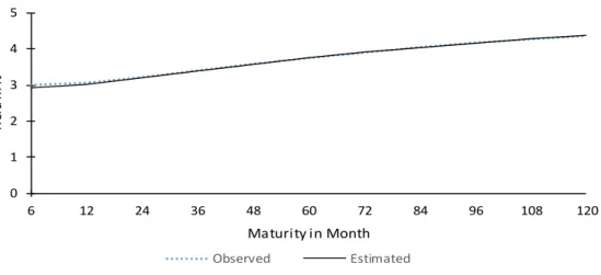
Afonso and Martins (2010) report similar results for the period 1972 to 2010 for Germany. The good in-sample fit is plotted in Figure 1 showing the observed and estimated yield curve. Only for the short-end one can see a deviation. For higher maturities, almost no difference can be identified. The average curve shows the typical upward sloped pattern.
Figure 1 Average estimated and observed yield curve
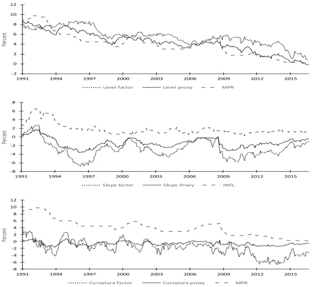
Before I discuss the estimation results, I want to provide evidence on the interpretation of the three latent factors as level, slope and curvature and I want to use basic statistic description to give a first economic interpretation of the three factors. In Figure 2, I show the estimated factors, its empirical proxies, and closest macroeconomic factors. As empirical proxies, I use [𝑌(120)] for the level, [𝑦(3) − 𝑦(120)] for the slope and [2 ∗ 𝑦(36) − 𝑦(120) − 𝑦(6)] for the curvature. For the level and the slope, a clear co-movement between the empirical proxies and the estimated factors can be seen. However, for the curvature, the clearness is not obvious, but one can still see a joint pattern with its empirical counterpart. The correlations support the interpretation of the three latent factors with coefficients of 𝜌(𝐿̂, 𝐿) = 0.91, 𝜌(𝑆̂, 𝑆) = 0.95 and 𝜌(𝐶̂, 𝐶) = 0.78.
From a macroeconomic perspective, the monetary policy rate can only directly impact the short-end of the yield curve. The relation for bonds of longer maturities is described by the expectation
0 1 2 3 4 5 6 12 24 36 48 60 72 84 96 108 120 Yi el d in % Maturity in Month Observed Estimated
16
Figure 2 Estimated level, slope and curvature, and its empirical proxies
hypothesis suggesting that yields of longer maturities are an average of the current and expected future short rates plus a constant term premium. In turn, the expected future short rates depend on expectations about future inflation and future real rates of return, which depend on economic activity (Lange, 2013). Regarding the term premium, newer research suggests a time-varying factor (Bauer et al., 2016).
Therefore, the impact of a current monetary policy change on the entire yield curve depends on its influence on expectations about future monetary policy rates / short rates being incorporated into long-term rates and its associated uncertainty if a time-varying term premium is assumed (Lange, 2013; Bauer, 2012). Hence, a monetary policy change may not only influence current economic activity or current inflation expectations but may also contain
-2 0 2 4 6 8 10 12 1991 1994 1997 2000 2003 2006 2009 2012 2015 Pe rc en t
Level factor Level proxy MPR
-8 -6 -4 -2 0 2 4 6 8 1991 1994 1997 2000 2003 2006 2009 2012 2015 Pe rc en t
Slope factor Slope Prox y INFL
-8 -6 -4 -2 0 2 4 6 8 10 12 1991 1994 1997 2000 2003 2006 2009 2012 2015 Pe rc en t
17
information to shape expectations about future inflation and future economic activity, termed the “expectation channel” (Geiger, 2011). These theories are not exclusive but may help to interpret the dynamics of the model.
For the German yield curve, all three factors are related to monetary policy with correlation coefficients of 𝜌(𝐿̂, 𝑀𝑃𝑅) = 0.72, 𝜌(𝑆̂, 𝑀𝑃𝑅) = 0.60 and 𝜌(𝐶̂, 𝑀𝑃𝑅) = 0.60. The first term supports the theory, that all yields should be somehow influenced by the monetary policy rate and that expectations of future short rates rates may depend on the current monetary policy rate. The co-movement with the level factor in the first panel of Figure 2 supports the interpretation. Lange (2013) finds similar evidence for Canada. The correlation with the slope and curvature suggests that yields of different maturities show varying reactions on monetary policy changes. Overall, the monetary policy rate appears an important driver of the German yield curve.
Furthermore, I also find evidence for a link between inflation and the level and slope factor with coefficients of 𝜌(𝐿̂, 𝐼𝑁𝐹𝐿) = 0.51 and 𝜌(𝑆̂, 𝐼𝑁𝐹𝐿) = 0.51. A close relation between yields and inflation expectations in economic theory is already described in the fisher equation. DRA (2006) also find a linkage between the level and the inflation. Overall, their close link appears to be widely accepted in the term structure literature (Afonso and Martins, 2010). Likewise, Lange (2013) also find evidence for the relation between the slope and inflation in Canada. I visualize the link for Germany in the second panel of Figure 2 for the slope factor. In contrast to DRA, I don’t find any closer link between the yield curve and industrial production based on correlation coefficients.
The upper part of Table 3 shows the results of the transition matrix A3. Again, all diagonal coefficients are significant at the 5 % level and highly persistent a typical pattern for Nelson-Siegel yield-macro models. Overall, 17 coefficients are significant at the 5 % level and 4 at the 0 % level. The estimated decay parameter of 0.0303 better fits bonds of longer maturities.
18
However, to facilitate interpretation I divide the A matrix into 4 3x3 blocks. 𝐴1, 𝐴2, 𝐴3 𝑎𝑛𝑑 𝐴4
contain the dynamics of lagged yield curve factors on current yield curve factors, lagged macroeconomic factors on yield factors, lagged yield curve factors on current macroeconomic factors and lagged macroeconomic factors on current macroeconomic factors, respectively:
𝐴 = [𝐴1 𝐴2 𝐴3 𝐴4]
The estimation results of block 𝐴1 suggest a more intense interaction between the three factors of the yield curve than in the yield-only model. Slope and curvature have a significant influence on next period’s level, but with less intense coefficients of -0.1 and 0.02, respectively. Level and slope reveal a significant impact on curvature, with high coefficients of 0.54 and 0.33. For the slope factor, I only find its own lagged coefficient as significant.
The second block reveals interesting insights on the different reactions of the yield factors on monetary policy changes and the different forces determining short and long-term bonds. The level is positively influenced by the monetary policy rate with a coefficient of 0.14 and significant at the 5 % level. It supports the previous interpretation that to some extent all yields should be shaped by a monetary policy change Also, it suggests that the current monetary policy rate influences expectations about future monetary policy rates / short rates, which is supported by the high persistence of the monetary policy time series.
The negative coefficient of -0.16 for the slope with a significance level of 10% decreases the short-end relative to the long-end of the yield curve and may increase the spread. However, the effect contradicts the usual assumption of a higher impact of a monetary policy tightening for short-term yields. Kato and Koeda (2010) suggest a higher term premium for bonds of longer maturity caused by a higher uncertainty due to a monetary policy change. Ireland (2015) finds a similar pattern for the term premium. Furthermore, the monetary policy change may lead to an increase in the inflation expectations (Lange, 2013), for example as a reaction to an overheating economy (DRA, 2006).
19 Table 3
Yield-Macro Model
VAR Transition Matrix A
Lt-1 St-1 Ct-1 IPt-1 MPRt-1 INFLt-1 µ Lt 0.81 -0.10 0.02 0.00 0.14 -0.01 4.84 0.05 0.04 0.01 0.00 0.05 0.03 3.70 St 0.14 1.06 0.03 0.01 -0.16 0.05 -2.55 0.10 0.07 0.02 0.01 0.08 0.04 1.14 Ct 0.54 0.33 0.88 -0.01 -0.33 -0.14 -1.91 0.13 0.09 0.03 0.01 0.11 0.07 3.47 IPt 0.77 0.42 0.19 0.92 -0.89 0.26 2.25 0.46 0.31 0.10 0.02 0.38 0.21 1.70 MPRt 0.11 0.09 0.03 0.01 0.87 0.01 3.21 0.04 0.03 0.01 0.00 0.03 0.01 4.36 INFLt 0.03 0.04 0.00 0.00 0.00 0.92 1.22 0.08 0.06 0.01 0.00 0.06 0.03 1.49
VAR Transition Covariace Matrix Q
Lt St Ct IPt MPRt INFLt Lt 0.07 -0.08 -0.08 -0.02 0.00 -0.01 0.09 0.01 0.02 0.03 0.00 0.01 St 0.17 0.06 0.05 0.01 0.02 0.08 0.02 0.06 0.00 0.01 Ct 0.48 0.00 -0.01 0.02 0.12 0.07 0.01 0.02 IPt 4.26 0.03 -0.08 0.08 0.02 0.05 MPRt 0.02 0.00 0.08 0.00 INFLt 0.09 0.06
Test for diagonality of Q matrix
P-Value
Wald test 164.54 0.00
Bold values represent estimates significant at th 5% level, underlined at the 10% level
20
However, the negative influence on next period curvature with a coefficient of -0.33 and significant at the 5 % level implies a relative decrease in middle-range yields after a monetary policy rate increase. A possible argument here may be that an increase in the monetary policy rate is often followed by an economic downturn (DRA, 2006 and Geiger, 2011). In addition, inflation could be lowered if the central bank has a reliable reputation regarding price stability contradicting the last argument for the slope. In particular, this effect is assumed to take place with an adequate time-lag, hence, decreasing relatively bonds of middle/longer maturities compared to the short-end (Geiger, 2011). However, well-anchored inflation expectations in the long-run and a Central Bank with a reputation of fighting against inflation are in favor of the curvature argumentation (Ehrmann et al., 2007; Hayo and Hofmann, 2005).
Overall, the results reveal a significant link from monetary policy to the yield curve. Therefore, decision-makers in Germany may be provided with a powerful tool, since the monetary policy rate can influence all three factors and thus has an impact on the entire maturity spectra of the yield curve and not only on the short-end. Hence, also bonds of longer maturity may be influenced being an important determinant for consumption and investment decisions (Geiger, 2011). Simultaneously, the result suggests that the monetary policy should contain information for the yield curve of the next period and may be exploited to improve forecasts for the term structure.
However, the opposing reactions to a monetary policy change reveal a complicated and complex transmission mechanism, since yields of different maturities can move in different directions. Therefore, it could be helpful for central banks to identify the varying pass-through channels of the monetary policy rate and to consider the asymmetric responses of the yield curve in its decision process. Also, the estimation results indicate monetary policy as an important driver of the yield curve. Hence, an anticipatable monetary policy may have the potential to reduce uncertainty about the yield curve and to create a more stable environment.
21
The positive but small effect of industrial production with a coefficient of 0.01 on the slope is in line with an interpretation of a monetary policy regime reacting with a tightening to an economic output growth and trying to increase the short-end of the yield curve to cool-down the economy (DRA, 2006).
The negative effect of inflation on the curvature with a coefficient of -0.14 is on the one hand contractionary to common perceptions about the reaction of middle/long-term yields to an increasing inflation, but on the other hand partially in line with previous findings. An increase in inflationary pressure may be followed by an aggressive intervention of the central bank, resulting in an economic downturn and opposed effects on nearby future inflation expectations. In block 𝐴3 lagged slope and curvature have a positive impact on industrial production significant at the 10% level with coefficients of 0.77 and 0.19. Following the efficient market hypothesis market participants may incorporate all information available and sense next period production dynamics. Hence, swings in both factors may represent a change in industrial production and could be used as a monitoring tool to capture economic activity dynamics.
Further in the third block, level, slope and curvature have a significant effect on the monetary policy rate in the next period with coefficients of 0.11, 0.09 and 0.03, respectively. Since the Canadian yield curve reveals a similar pattern, Lange (2013) offers two possible interpretations. On the one hand, the yield curve could move due to an anticipation of the monetary policy reaction on new economic data, which implies forward looking market participants and a next period’s monetary policy rate being transparent and anticipatable. On the other hand, monetary policy could adjust its main rate to new financial market data aggregated in the yield curve.
However, central bankers (and market participants) can obtain important information about the market expectations for the monetary policy in the next period from the yield curve and may use it as a monitoring tool. Therefore, the monetary policy regime could conduct a policy smoothed towards market expectations with the potential to stabilize the economy. Overall, the
22
close interaction between monetary policy and the yield curve factors in block A2 and A3 suggests a strong bidirectional relation between both.
However, the yield curve seems to contain no information on next period’s inflation. Lange (2013) receives a similar result for Canada.
Block 𝐴4 completes the picture. Lagged monetary policy rate decreases industrial production almost one on one with a high coefficient of -0.89. Vice versa, growing industrial production increase the monetary policy in the next period by 0.01. Both are in line with previous explanations. The monetary institution responds with a tighter policy to a growing industrial production, and on the other hand, tighter policy leads to an economic downturn. Thus, a monetary policy regime not only needs to consider the opposing effects on the yield curve but also the effect on economic activity in its decision process. Simultaneously, the result suggests that at least in the short-run monetary policy can influence economic activity. Also, the result could be an indicator for a forward-looking monetary policy, as it reacts to expected inflationary pressure due to a growing industrial production.
The lower part of Table 3 shows the Q matrix of the yield-macro model. Again, all diagonal coefficient and 5 of the covariance terms are significant. All covariances of the yield curve factors are significant at the 5% level supporting the previous view of a complex interaction between them. It’s interesting, that again the link between the slope and the monetary policy is significant supporting the findings of a closer connection between the two factors. Further, the covariance between the slope and the inflation is significant. Only five significant covariances could suggest a restricted diagonalized covariance matrix. However, I test this assumption by applying a Wald test to assess the hypothesis of diagonality showed in the lowest part of Table 3. The test clearly rejects the hypothesis supporting the choice of the model.
To complete the analysis, I also conduct Wald tests to evaluate the joint non-zero unidirectional effects of the yield factors on the macroeconomic factors (A3 = 0, Q2 = 0), vice
23
versa (A2 = 0), and bidirectional effects (A3 = 0, Q2 = 0, A2 = 0) presented in Table 4. 𝑄2
refers to the upper right 3x3 block consisting of the covariance terms between macroeconomic and yield factors. I follow DRA and attribute 𝑄2 to the effects the yield factors exercise on the macroeconomic factors due to the ordering of the VAR (1).
Table 4
Wald-tests for macro/yields interaction
All three tests reject the zero-interaction hypothesis. Hence, I find clear evidence for interactions between macroeconomic factors and the yield curve in both directions. In particular, a bidirectional link is supported.
In Table 2, I also compute the residuals of the estimated yields for the yield-macro model. They are almost identical to the yield-only model, also suggesting a very good overall in-sample fit. DRA find a likewise symmetry between the measurement errors of both models. Hence, all highlights mentioned for the yield-only model above apply to the yield-macro model as well. Also, the time series for the latent factors and the yields are almost identical for the estimated yield-only and yield-macro model.
5. Conclusion
Using a dynamic Nelson-Siegel model to represent the term structure of interest rates the dynamics of the German yield curve can be fitted very well. Also, the interpretation of the three factors as level, slope and curvature appears reasonable for the German curve. I also receive a typical pattern for measurement errors with almost negligible errors for the middle range.
No interaction (A2=0,A3=0,Q2=0) No macro to yields (A2=0) No yields to macro (A3=0,Q2=0)
# restrictions Test statistics P-Value
9 30.02 0.00
18 133.91 0.00
24
Further, I find strong evidence for a bidirectional relationship between macroeconomic factors and the yield curve in Germany. Monetary policy exercises a significant effect on all yield curve factors revealing a powerful tool for the monetary policy regime to influence the entire yield curve. At the same time, all three yield curve factors have a significant influence on the monetary policy rate implying forward-looking market participants. Simultaneously, the results also suggest information contained in the yield curve about next period’s industrial production growth. Therefore, the German yield curve may serve as a monitoring tool for both: industrial production dynamics and monetary policy expectations. Less influence from the inflation to the yield curve and vice versa was found. Also, the results imply an intense influence of the monetary policy rate on economic activity in the next period.
Overall, the results indicate a strong bidirectional relationship between the yield curve and the monetary policy rate in Germany.
However, future research could deepen the analysis by assessing impulse response functions and variance decomposition to understand surprising changes. A decomposition of the yields in an expected and term premium component could help market participants and central bankers to better understand the pass-through channels of monetary policy and their impact on the entire maturity spectra.
References
Afonso, António & Martins, Manuel M.F. 2010. "Level, slope, curvature of the sovereign yield curve, and fiscal behaviour." Working Paper Series 1276, European Central Bank: 1-63.
Ang, A. and Piazzesi, M. 2003. "A no-arbitrage vector autoregression of term structure dynamics with macroeconomic and latent variables." Journal of Monetary Economics, 50: 745-787.
Bauer, M. D. and Hamilton J. D. 2016. "Do Macro Variables Help Forecast Interest Rates ?" FRBSF Economic Letter, 2016-20: 1-5.
Bauer, M. D. 2012. "Monetary Policy and Interest Rate Uncertainty." FRBSF Economic Letter, 2012-38: 1-5.
Dai, Qiang and Singleton, Kenneth J. 2000. "Specification Analysis of Affine Term Structure Models." Journal of Finace, 55: 1943-1978.
25
Diebold, F.X. and Rudebusch, G.D. and Aruoba, Boragan. 2006. "The macroeconomy and the yield curve: a dynamic latent factor approach." Journal of Econometrics, 131: 309-338.
Diebold, F.X. and Rudebusch, G.D. 2013. Yield Curve Modeling and Forecasting: The Dynamic Nelson-Siegel Approach. Princeton University Press.
Diebold, Francis and Li, Canlin. 2005. "Forecasting the term structure of government." Journal of Econometrics, 130: 337-364.
Duffee, Gregory R. 2002. "Term Premia and Interest Rate Forecasts in Affine Models." Journal of Finance, 57: 405-443.
Durbin, J. and Koopman, S. J. 2012. Time Series Analysis by State Space Models. Oxford University Press.
Ehrmann, M. and Fratzscher,M. and Gürkaynak, R.S. and Swanson, E.T. 2007. "Convergence and anchoring of yield curves in the Euro area." Working Paper Series, European Central Bank, 817: 1-52.
Estrella, A., and Hardouvelis, G.A. 1991. "The Term Structure as a Predictor of Real Economic Activity." Journal of Finance, 46: 555-576.
Geiger, Felix. 2011. The Yield Curve and Financial Risk Premia. Springer.
Hayo, B. and Hofmann, B. 2005. "Comparing Monetary Policy Reaction Functions: ECB versus Bundesbank." Marburg Economics Working Paper No. 02-2005: 1-23.
Hördahl, Peter and Tristani, Oreste and Vestin, David. 2006. "A Joint Econometric Model of Macroeconomic and Term Structure Dynamics." Journal of Econometrics, 131: 405-444.
Ireland, Peter N. 2015. "Monetary Policy, Bond Risk Premia, and the Economy." Journal of Monetary Economics, 76: 124-140.
Koeda, J. and Kato, R. 2010. "The Role of Monetary Policy Uncertainty in the Term Structure of Interest Rates ." IMES Discussion Paper Series, 2010-E-24: 1-37.
Koopman, J.S. and Mallee, M.I.P and Van der Wel, Michel. 2007. "Analyzing the Term Structure of Interest Rates using the Dynamic Nelson-Siegel Model with Time-Varying Parameters." Tinbergen Institute Discussion Paper, 095/4: 1-41.
Lange, Ronald H. 2013. "The Canadian macroeconomy and the yield curve: A dynamic latent factor approach." International Review of Economics and Finance, 27: 261-274. Levant, Jared and Ma, Jun. 2016, 37:. "Investigating United Kingdom's monetary policy with
Macro-Factor Augmented Dynamic Nelson–Siegel models." Journal of Empirical Finance 117-127.
Litterman, R. and Scheinkman, J. 1991. "Common factors affecting bond returns." Journal of Fixed Income, 1: 54-61.
Nelson, C.R., Siegel, A.F. 1987. " Parsimonious modeling of yield curve." Journal of Business, 60: 473-489.
Rudebusch, G.D. and Svensson, L.E.O. 1999. "Policy rules for inflation targeting. Monetary Policy Rules." University of Chicago Press 203–262.
Rudebusch, Glenn D. and Tao Wu. 2008. "Macro-Finance Model of the Term Structure, Monetary Policy, and the Economy." Economic Journal, 118: 906-926.
Wheelock, D. and Wohar M. 2009. "Can the term spread predict output growth and
recessions? a survey of the literature." Federal Reserve Bank of St. Louis, issue Sep: 419-440.