GDP-linked bonds : design, effects, pricing and way forward

! "!

GDP-Linked Bonds

Design, effects, pricing and way forward

Author

David Miguel Taylor de Jesus Marques Pereira

Supervisor

Diana Bonfim

Dissertation submitted in partial fulfillment of requirements for the degree of

Master in Finance, at the Universidade Católica Portuguesa, 18 April 2017

! #!

ABSTRACT

!

GDP-linked bonds could play an important role in helping countries to avoid solvency crises, defaults and sovereign debt restructurings. Indexing a country’s debt payments to its economic performance could give governments some type of insurance against periods of declining growth rates.

In this context, this thesis illustrates the potential advantages of the issuance of such an instrument, namely by quantifying the above mentioned insurance effect. As such, the interest savings for a group of countries most affected by the European sovereign debt crisis should they have issued GDP-linked bonds in the beginning of the decade are calculated. It is concluded that theses savings would have been considerable. Furthermore, in order to understand the additional room for countercyclical fiscal measures created by this product, the correlation between primary balance and GDP growth is simulated for both scenarios: debt with indexation to GDP growth and without it. It is then concluded that correlation between those two variables would be significantly higher with indexation.

In the same vein, it is also simulated the issuance of this instrument in currency unions, in particular in the euro area, applying the corresponding fiscal constraint to the total deficit of 3% of GDP. Thus, the correlation between primary balance and GDP growth shows that indexing debt to GDP growth has the potential to offset the curbing effect of the mentioned constraint.

Moreover, through simple regressions and using the Capital Asset Pricing Model, it is concluded that the portion of undiversified risk associated to the indexation to GDP growth would be low.

! ##!

ACKNOWLEDGEMENTS

!

I would like to acknowledge the guidance of Prof. Diana Bonfim during the thesis elaboration process, in particular her availability to discuss and helping to find the best solutions.

I also thank my family, friends and colleagues for their support and encouragement in pursuing this degree.

! !

! ###!

TABLE OF CONTENTS

3.1.! _{Design – The coupon formula'((((((((((((((((((((((((((((((((((((((((((((((((((((((((((((((((((((((((((((((((((((((('N}!

3.2.! _{Fiscal Effects of GDP-linked bonds'((((((((((((((((((((((((((((((((((((((((((((((((((((((((((((((((((((((((((((('O}!

3.2.1.! _{Interest bill savings/expense!$$$$$$$$$$$$$$$$$$$$$$$$$$$$$$$$$$$$$$$$$$$$$$$$$$$$$$$$$$$$$$$$$$$$$$$$$$$$$$$$$$$$$$$$$$$$$$$$!%}! 3.2.2.! _{Fiscal policy!$$$$$$$$$$$$$$$$$$$$$$$$$$$$$$$$$$$$$$$$$$$$$$$$$$$$$$$$$$$$$$$$$$$$$$$$$$$$$$$$$$$$$$$$$$$$$$$$$$$$$$$$$$$$$$$$$$$$$$$$$$$!"&}!

3.2.2.1.! _{Avoiding procyclical fiscal measures!$$$$$$$$$$$$$$$$$$$$$$$$$$$$$$$$$$$$$$$$$$$$$$$$$$$$$$$$$$$$$$$$$$$$$$$$$$$$$$$$$$$!"&}!

3.2.2.2.! _{Introducing fiscal constraints!$$$$$$$$$$$$$$$$$$$$$$$$$$$$$$$$$$$$$$$$$$$$$$$$$$$$$$$$$$$$$$$$$$$$$$$$$$$$$$$$$$$$$$$$$$$$$$$$$$$!"'}!

3.3.! _{Pricing - Indexation Premium'(((((((((((((((((((((((((((((((((((((((((((((((((((((((((((((((((((((((((((((((((((('=P}!

Q(! D8>@)9;I')II;?6<>IK'H?88)>8I'79')RMF>R>67?7)96'?6:'M9II)HF>'I9F;7)96I=Q!

4.1.! _{Previous issuances of sovereign’s equity-like instruments'((((((((((((((((((((((((((((((((((('=S}!

4.2.! _{Barriers to implementation and possible solutions'(((((((((((((((((((((((((((((((((((((((((((((((('=N}!

S(! &96<F;I)96I'(((((((((((((((((((((((((((((((((((((((((((((((((((((((((((((((((((((((((((((((((((((((((((((((((((((((((((((('BP! .)I7'9L'L)C;8>I'(((((((((((((((((((((((((((((((((((((((((((((((((((((((((((((((((((((((((((((((((((((((((((((((((((((((((((((((((('B=! .)I7'9L'7?HF>I'(((((((((((((((((((((((((((((((((((((((((((((((((((((((((((((((((((((((((((((((((((((((((((((((((((((((((((((((((((('B=! .)I7'9L'>T;?7)96I'((((((((((((((((((((((((((((((((((((((((((((((((((((((((((((((((((((((((((((((((((((((((((((((((((((((((((((('B=! ")HF)9C8?MUV'((((((((((((((((((((((((((((((((((((((((((((((((((((((((((((((((((((((((((((((((((((((((((((((((((((((((((((((((((('BB!

! "!

1. Introduction

Debt restructurings - which recently also occurred in advanced economies - and its effects have long been a concern for sovereign bonds investors and researchers, having witnessed a peak of interest during the recent global financial crisis. As such, most of the restructurings so far took place after default and are usually described as having harmful consequences on the domestic economy and the financial sector (Trebesch et al. 2012), and those that include higher haircuts can translate into higher bond yield spreads and extended periods of capital markets exclusion (Cruces & Trebesch 2013).

In this context, and given the specific features of restructurings with sovereign involvement versus private sector, new forms of debt instruments have been suggested in order to make them more efficient. In particular, against a background of countries with high levels of debt, coupled with low levels of growth and inflation, GDP-linked bonds have been recently in the spotlight. The G-20, in the G20 Finance Ministers and Central Bank Governors Meeting of 24 July 2016, recognized that fiscal policy and fiscal strategies are essential in supporting growth. As such, G-20 members, in that meeting’s communiqué, called for “further analysis of the technicalities, opportunities, and challenges of state-contingent debt instruments, including GDP-linked bonds (…)” (G20 2016).

The particular characteristic of a GDP-linked bond is the indexation of its coupon rate (or even its principal) to the issuer country’s GDP growth rate so that the security’s cash flow payments would reflect and adjust to the GDP evolution. This debt instrument could play an important role in helping to avoid solvency crises by,

inter alia, increasing countries’ fiscal space and allowing for countercyclical fiscal

policies, providing countries with a form of insurance against downturns. It would, therefore, reduce the probability of defaults, debt restructurings and their associated costs. Researchers have been exploring GDP-indexed bonds since the 1990s and instruments with growth performance indexation features have already been issued (for instances by Costa Rica, Bulgaria, Bosnia Herzegovina, Singapore, and more recently by Argentina and Greece and Ukraine). However, this type of issuance is

! (! still considered an exception and has not accomplished its full potential as an instrument that could play an important role in helping countries to avoid solvency crises and by better sharing risk with private creditors.

As such, first, this thesis depicts the main characteristics of a GDP-indexed bond (section 1.1) and, in order to quantify its insurance effect and to understand other potential fiscal benefits, a set of scenarios are presented, revisiting some of the exercises laid out by Borensztein and Mauro (Borensztein & Mauro 2004). In section 1.2.1 the savings or expenses are calculated, between 2000 and 2013, for a group of countries (Portugal, Spain and Ireland) should they have issued GDP-indexed bonds. By adjusting the implicit observed coupon rate to growth performance, a new rate is calculated and the difference between the corresponding interest amounts is computed so that the mentioned savings or expenses could be determined.

In section 1.2.2, also simulating that a group of countries had issued this growth-indexed instrument, it is illustrated how much additional room countries would have had to pursue countercyclical fiscal policies. This is achieved by calculating, for the period between 2000 and 2013, the correlation between primary balance and growth rate in two scenarios: with plain vanilla bonds and introducing GDP-linked bonds. In the latter case, an “adjusted primary balance” is computed considering the new interest amounts stemming from the introduction of the new instrument. In section 1.2.3 that same additional room is simulated, for the same period, in the case of a fiscal deficit limit of 3% of GDP.

In section 1.3, we estimate the possible impact of the indexation of the coupon rate to GDP growth on the interest rate, in particular on how much above the risk-free rate would investors ask for holding this kind of growth performance instrument. As such, a set of regressions (for the period 1980-2015) of individual countries’ GDP growth rates on the world real GDP rates was estimated in order to assess the associated undiversified risk.

Finally, in section 2, previous issuances of GDP-linked instruments are analysed (section 2.1) and, in section 2.2, barriers to the implementation of such a product and possible solutions to overcome them are discussed.

! )!

2. Literature Review

The international debt crisis in the 1980s led countries to fail their legal obligation to meet debt repayments in many countries worldwide, in particular in Latin America and Eastern Europe. Ever since then, both experts and researchers have been interested in finding instruments that improve risk-sharing arrangements between governments and investors, allowing for a reduction of sovereign defaults and their corresponding costs. In this context, proposals of innovative financial products began to emerge, including the suggestion of indexing debt repayments to macroeconomic variables such as GDP, exports or commodity prices. As an example, Krugman (Krugman 1988), in an attempt to solve the trade-off between debt forgiveness and financing, suggested that linking payments to measures of economic conditions could benefit both debtors and creditors.

Nevertheless, to understand better the importance of these types of instruments, it is crucial to describe the broader context in which they assume relevance. In this vein, the usual length and complexity of sovereign debt restructurings must be highlighted. As described by Trebesch et al., these processes are triggered by a default episode in contracted debt payments or by a debt-restructuring announcement (Trebesch et al. 2012). This is often when Governments start negotiation procedures with creditors, in order to agree on the terms of a debt exchange, which will provide debtors with debt relief. These processes can take several years.

Adding to the above-mentioned procedural complexity, there are specificities for sovereign debt restructurings, as opposed to for private sector processes, making them more difficult to achieve. Brooke and Mendes list the following characteristics: i) limits on the available legal means to enforce payments, namely the inability to liquidate the sovereign’s assets; ii) constraints on the ability of a sovereign to pledge collateral credibly; iii) the large size of individual stocks of sovereign debt which makes it difficult to hedge its default risk effectively; and iv) the importance of sovereign debt in financial markets (Brooke & Mendes 2013). Bedford et al. also stress the current poor coordination between creditors and sovereigns in debt restructurings and information asymmetries (Bedford et al. 2005).

! &! In this context and given the frequency of financial crises, particularly in emerging economies, several authors have suggested ways to reduce inefficiencies of debt restructurings and their consequential costs. Borensztein and Panizza investigate the empirical basis of the costs of sovereign defaults (Borensztein & Panizza 2009), and Eichengreen discusses different approaches to this problem, presenting three main possible reforms: i) maintaining the status quo, promoting the development of more complete and efficient debt agreements - a "contractual approach", falling under the currently used collective action clauses (CAC); ii) a "legislative approach" that would provide some of the functions of an international mechanism of insolvency; and finally iii) the establishment of a full-fledged international bankruptcy court (Eichengreen 2003).

With regard to the “legislative approach” (reform ii), Anne Krueger, former First Deputy Managing Director of the IMF, proposed in 2002 the creation of a sovereign debt restructuring mechanism, equitable across all the sovereigns’ creditors, allowing for an orderly, timely and predictable restructuring process of considered unsustainable debt"_{. Along the same lines, more recently, (Gianviti et al. 2010)}

proposed in 2010 the creation of a European Crisis Resolution Mechanism(_.

Nevertheless, the IMF, recognising and supporting the need for reforms in order to achieve more orderly sovereign debt restructurings, seems to follow the “contractual approach”, by reforming bond contracts (reform i).

Finally, Eichengreen suggested that those with reservations about these two approaches would want alternatives, such as new forms of debt (Eichengreen 2003). And, as a reference, quoted (Borensztein & Mauro 2002), who suggested debt instruments indexed to countries’ real growth rate of their own GDP as a way to self-insure against possible growth slowdowns.

!!!!!!!!!!!!!!!!!!!!!!!!!!!!!!!!!!!!!!!!!!!!!!!!!!!!!!!!

"

A New Approach to Sovereign Debt Restructuring, Anne O. Krueger, International Monetary Fund, 2002 ((Krueger 2002)).

(

In the context of reducing uncertainty regarding sovereign debt restructuring processes, (Amador et al. 2016), while mentioning the main proposals for default mechanisms presented so far, argue that “three characteristics may be considered decisive” for the effective operation of insolvency mechanisms (in particular, clear definition of the events which trigger the process, minimisation of the “holdouts” amounts and its implementation should not be undermined by, for example, “the utilisation of other types of debt or amendments to the rules”.

! *! Moreover, Brooke and Mendes argue that the current approach to sovereign debt restructurings is “sub-optimal” (Brooke & Mendes 2013). They highlight five main reasons: i) it increases the risk of moral-hazard; ii) it incentivises short-term lending; iii) the risk to taxpayers’ resources; iv) the greater difficulty in the negotiation of debt write-downs, given substantial official sector debt holdings; and v) the delay of necessary reforms, which will require substantial policy adjustments when intervention is eventually needed (“gambling for redemption”). These authors proposed contractual reforms to sovereign debt contracts in order to improve crisis prevention and resolution, suggesting higher risk sharing between sovereigns and private creditors. Accordingly, they proposed the introduction of two complementary types of state-contingent bonds: ‘sovereign cocos’ and ‘GDP-linked bonds’. The first would reduce the probability of solvency crises and the second serve to cover liquidity crises.

Research on GDP-linked bonds seems to date back to the early 1990s with a proposal from Shiller (Shiller 1993), who defended a market for long-term claims on the major aggregate income flows: gross domestic product, occupational income, and service flows from commercial and residential real estate. Furthermore, he argued that instruments whose payments are linked to GDP could help reduce country risk and promote welfare.

Borensztein and Mauro argue that GDP-indexed bonds, by keeping the debt/GDP ratio within a narrower range than plain vanilla bonds, could play a role in preventing future debt crises, representing a way for countries to self-insure against possible growth downturns (Borensztein & Mauro 2002; Borensztein & Mauro 2004). They also suggest that official intervention in the setting-up of the corresponding market could help overcome some of the obstacles to its implementation. Furthermore, it is illustrated how this product could reduce the need for countries to conduct pro-cyclical fiscal policies and their benefits for countries that belong to economic monetary unions. Finally, they also conclude that the insurance premium, that is the risk premium for holding bonds indexed to GDP, compensating investors for GDP volatility, would be small. In order to evaluate how markets would price this instrument, they use, as a starting point, the Capital Asset Pricing Model (CAPM).

! +! As concerns pricing, and maintaining that GDP-indexed bonds are not much more difficult to price than plain-vanilla bonds, Chamon and Mauro (Chamon & Mauro 2006) introduced the risk of default into their model. Firstly, they extracted different combinations of probabilities of default and recovery rates from observed yields. Then, using the Monte Carlo framework, they simulated several paths for economic variables and debt/GDP ratio. Afterwards, they obtained a default trigger for the debt/GDP ratio and recovery rate that would yield the expected repayments implicit in the spreads. Finally, using the debt/GDP ratio default trigger and the simulated paths for the economic variables, they computed the corresponding payoff for both the growth-indexed bonds and the standard plain-vanilla bonds. The authors concluded that GDP-indexed debt can lower default frequency and when the share of this type of debt increases, both plain-vanilla and growth-linked bonds become less sensitive to GDP volatility and to growth shocks.

Miyajima (Miyajima 2006) evaluates GDP-linked warrants (GLWs) considering the issuer’s repayment capacity in the pricing formula. The author estimates the expected cash flows of debt payments, assuming that GDP follows a stochastic model, while trigger conditions are also modelled using the Monte Carlo framework. The issuer’s capacity to service debt is defined as the difference between the incremental payments of GLWs and the increases in tax revenues due to economic growth. Finally, (Miyajima 2006) also uses CAPM to calculate the size of the indexation premium, also finding it to be low (“lower than the results in the literature”).

Sharma and Griffith-Jones (Sharma & Griffith-Jones 2009) discuss the benefits of introducing GDP-linked bonds to borrowing countries, investors and to the global economy and financial system, while presenting the main concerns, issues and obstacles to their implementation. They also present recent experiences with these types of bonds, explaining their major flaws. Finally, in the same vein as Borensztein and Mauro (Borensztein & Mauro 2004), the authors also recognise the case for international public intervention to help develop a specific market, suggesting several steps forward to this end.

Kamstra and Shiller (Kamstra & Shiller 2009) propose a particular type of GDP-linked bond, a security with a coupon indexed to the United States’ current dollar GDP, that would pay, for example, one-trillionth of the GDP. The maturity of this

! ,! security would be long term, preferably perpetual. They consider that this new instrument would perform an important role as a stabiliser of the public budget. Finally, the authors also use CAPM to calculate the cost of capital “relevant to issuing Trills”, culminating in a risk premium of “only” 1.5 percent.

Recently, Barr et al. (Barr et al. 2014) have presented a model of endogenous sovereign default, in which they analyse how GDP-linked bonds can raise the maximum sustainable debt level of a government and reduce the incidence of defaults. They use the concept of fiscal fatigue and standard debt dynamics equations to estimate debt limits, which will then be determinant to model sovereign default with plain-vanilla and GDP-linked bonds. Under different risk aversion scenarios, the introduction of this security would increase the debt-limit level. In spite of this, investors demand a premium for providing insurance against GDP volatility. As the debt/GDP ratio increases, this specific cost gets overturned as default premium increases.

Finally, Benford et al. (Benford et al. 2016) distinguish between GDP-linked bonds’ issuances in normal and in debt restructuring times, with different benefits for issuers. During normal times it would help in preventing solvency crises, giving more fiscal space in downturns. In restructurings, this instrument would allow transferring higher debt repayments to when growth is recovering.

3. Introducing GDP-linked bonds – Design, effects and pricing

3.1. Design – The coupon formula

The specific feature of a GDP-linked bond is the indexation of its coupon rate to the issuer country’s GDP growth rate so that the security’s cash flow payments would reflect and adjust to the GDP evolution. In other words, the debt redemption’s value would reflect the country’s growth performance. If a government only issues this type of bond, all of its debt payments will change in line with growth.

A GDP-linked bond coupon rate would equal:

! '!

Equation 1

!

Specifically, in order for the coupon rate) _{to reflect the evolution of the GDP growth}

rate, an indexation factor, which would correspond to the difference between the observed growth rate (gt) and a baseline growth rate ( ), would be added to the

baseline coupon rate (r), thus linking coupon payments to the mentioned economic performance. This baseline growth rate, to be agreed at the moment of the contract&_,

would reflect a trend growth rate and would adjust the economic performance of the year t to a period of growth of sufficient length. As such, if the economy in year t grows above the baseline growth rate, the indexation factor would be positive and the coupon rate would be higher than the baseline coupon rate. If the economy grows below the baseline, the indexation factor would be negative and the coupon rate would be lower than r. Finally, in order to protect investors from periods of particularly weak economic performance – when, by adjusting the baseline coupon rate to a sufficiently negative indexation factor, the coupon rate would be negative – and thus also avoiding disincentives to investments in this kind of performance-linked security, a minimum of 0 would be applied to the coupon rate formula.

Therefore, the indexation of a bond to a country’s economic performance would give governments a certain degree of insurance against periods of declining growth rates (to the extent that coupon payments are more or less sensitive to growth * _and

depending on the maturity of the bond+_).

3.2. Fiscal Effects of GDP-linked bonds

!!!!!!!!!!!!!!!!!!!!!!!!!!!!!!!!!!!!!!!!!!!!!!!!!!!!!!!!

) _{For simplicity and in order to avoid another layer of risk, only the coupon rate – and not the}

principal – is adjusted.

& _{Borensztein and Mauro defend that the baseline growth rate of GDP would be agreed “upon by the}

contracting parties prior to the bonds’ issue” (Borensztein & Mauro 2004).

* _{Borensztein and Mauro defend that the “higher the elasticity of bond payments with respect to}

changes in economic growth, the higher the insurance of the government” (Borensztein & Mauro 2004). In this context, they note that the introduction of a positive minimum coupon payment reduces insurance and present other coupon formulas where a parameter ! is added to control the elasticity of

the coupon payment to the growth rate (e.g. !"#$"%!! !"# !!! ! !"# !! !!! !! ! !! ; where !!

is an adjustable benchmark growth rate and !! _{a maximum coupon payment).}

+ _{According to Barr et al., GDP-linked bonds with longer maturities give sovereigns a better hedge}

against lower trend growth (Barr et al. 2014). As an example, perpetual GDP-linked bonds would hedge all the debt against those shocks.

! %! In order to quantify the insurance effect and to understand other potential fiscal benefits of GDP-linked bonds, a set of scenarios are presented, following some of the exercises laid out by Borensztein and Mauro (Borensztein & Mauro 2004). In section 1.2.1 “interest bill savings/expenses”, the savings or expenses are calculated for a group of countries (Portugal, Spain and Ireland) should they have issued GDP-indexed bonds; in section 1.2.2 “avoiding procyclical fiscal measures”, also simulating that (a larger) group of countries had issued this growth-indexed instrument, it is illustrated how much additional room countries would have had to pursue countercyclical fiscal policies. Finally, in section 1.2.3 “introducing fiscal constraints”, that same additional room is simulated in the case of a fiscal deficit limit of 3% of GDP.

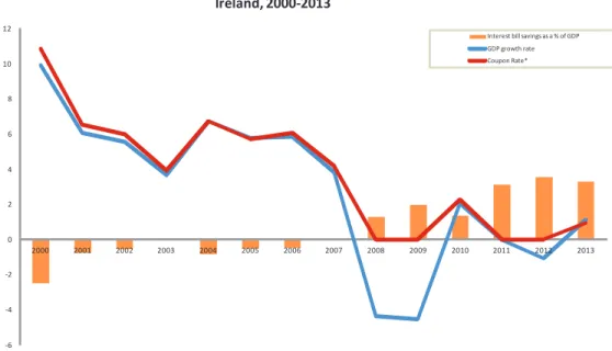
Data used, its description as well as its sources are described in Table 1 below.

Data Description Source

GDP growth rate, real

Gross Domestic Product, constant prices, annual percentage change

IMF Primary balance Primary balance as a percentage of GDP; annual

frequency

IMF Overall balance Overall balance as a percentage of GDP; annual

frequency

IMF Interest Gross interest (paid) as a percentage of GDP; annual

frequency

IMF Debt General government gross debt; percentage of GDP IMF

Table 1 Data description and sources

!

3.2.1. Interest bill savings/expense

!

This first exercise is an attempt, through a rather simple approach, to illustrate how GDP-indexed bonds could affect a sovereign’s interest bill. Following Borensztein and Mauro (Borensztein & Mauro 2004), it is employed a floating-rate bond with a coupon rate that follows a country’s economic performance.

In this context, using equation 1 presented in 1.1, a new coupon rate is simulated and, accordingly, the amount of interest savings (or expenses) accumulated (or incurred) if, since the beginning of 1999, all the government debt of some of the European countries most affected by the recent sovereign debt crisis - Portugal, Ireland and Spain - consisted of GDP-linked bonds. It is also assumed that the new coupon rate and interest bill would have no impact on other variables, such as GDP, total deficit

! "-! or debt, which, although unrealistic, is a good indicator of the expected potential amount of interest savings or expenses. Moreover, the baseline growth rate used corresponds to the average growth rate in the period 1980-2013, which, according to (Borensztein & Mauro 2004), “could be viewed as a mix of adaptive expectations and perfect foresight” ,; and should be long enough to provide a representative figure of the growth trend of a country. As regards GDP growth, it was chosen data in real terms, i.e. adjusted for inflation effects. It is arguable that GDP in nominal terms (as suggested by Benford et al. (Benford et al. 2016)) would protect investors also from inflation fluctuations, however, it seems more prudent (at least in a first period of issuance) to spare both investors and issuers of another layer of complexity and risk and focusing on the countercyclical potential effect of GDP-linked bonds.

As such, the actual implicit coupon rate is determined as a result of the ratio of gross interest payments of year t to the average of that same year’s debt and the one of year

t-1. However, it should be noted that this ratio does not consider that the actual debt

stock also includes other instruments (such as currency and deposits and loans). Also, one should take into account that countries that were under financial assistance were excluded from the bond market, contributing for a less meaningful coupon rate. The difference between that year’s GDP growth rate and the baseline growth rate is then added (or subtracted) to the coupon rate and the maximum of the adjusted coupon rate and 0 is computed. The new interest amount can thus be determined by applying that new coupon rate to the same average of year t and year t-1 debt.

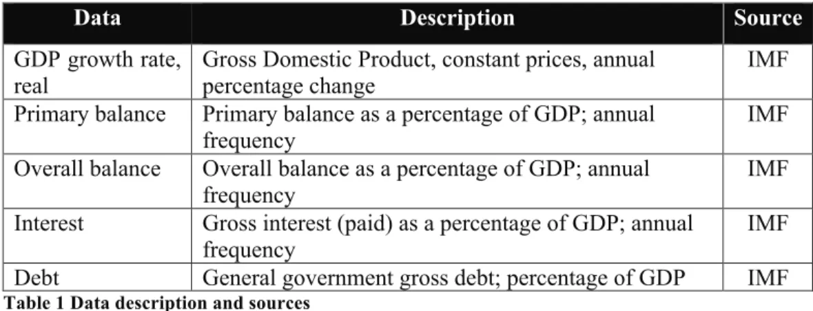
In the case of Portugal, the baseline growth rate would be 2.2%, which compares to a rather low average growth rate of around 0.3% in the more recent period 2000-2013 (Figure 1). This would suggest that, had the Portuguese government issued GDP-linked bonds, it would have paid an average coupon rate of around 3.0%, which is lower than the average observed (coupon) rate of around 4.5%.

In relatively good years - when the growth rate was higher than the baseline - the government would have incurred comparatively higher interest costs. This would have happened only in 2000 and in 2007. Conversely, in periods when the GDP !!!!!!!!!!!!!!!!!!!!!!!!!!!!!!!!!!!!!!!!!!!!!!!!!!!!!!!!

, _{Although asserting that economic agents have perfect foresight is a strong assumption, it allows for}

the consideration of expectations. However, this assumption has limited impact in this and the following exercises given that growth expectations are the same regardless of the fiscal policy adopted.

! ""! growth rate was below the baseline, the adjusted coupon rate would have been lower than the observed one, resulting in (the emergence of) interest savings. In periods of particularly low growth, including periods of negative growth rates, for instance from 2007 onwards (excluding 2010), the GDP-indexed debt would have translated into significant interest savings. This period coincided with the European sovereign debt crisis. The reduction in the government’s interest bill (amounting to around 1.4% of GDP during the period from 2000 to 2013) would have left room to avoid or minimize procyclical fiscal measures. The amount of savings generated could have been particularly useful for this country, in light of the significant fiscal and macroeconomic adjustment pursued during this period.

Figure 1 Interest savings over the economic cycle 2000-2013 – Portugal

The circumstantial value that GDP-linked bonds could have yielded to Portugal can be extended to other European countries, also heavily affected by the European sovereign debt crisis, such as Spain and Ireland.

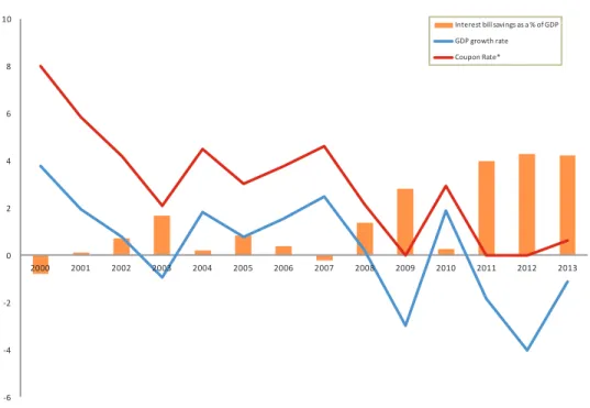
In Spain (Figure 2), a particularly poor economic performance period can be observed from 2008 onwards, with negative growth rates in 2009 and in the period 2011-2013 (in 2010 the GDP growth rate was close to zero). In this period (2008-2013), GDP-indexed bonds would have generated significant interest savings

!" !# !$ % $ # " & '% $%%% $%%' $%%$ $%%( $%%# $%%) $%%" $%%* $%%& $%%+ $%'% $%'' $%'$ $%'( !"#$%&'()*+,,,-+,./ ,-./0/1.2345521674-8126126292:;2<=> <=>280:?.@206./ A:BC:-2D6./E

! "(! compared to the amount of interest effectively paid, representing a saving of around 2.3% of GDP. From 2009 onwards (when the growth rate declined to around -3.6%), coupon rates would actually fall to their minimum level of zero. For the all sample period, considering also years when GDP growth was relatively high and stable, interest savings amounted to around 1.0% of GDP.

!

Figure 2 Interest savings over the economic cycle 2000-2013 – Spain

!

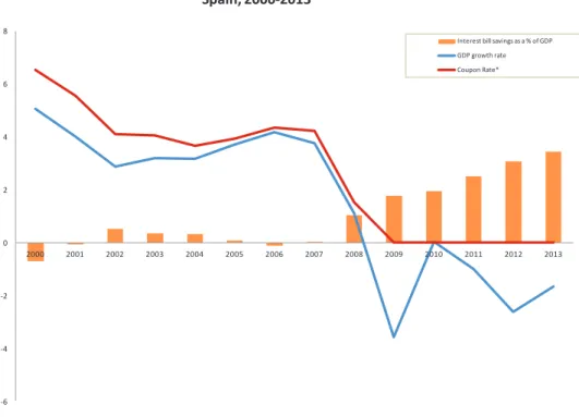
Finally, Ireland (Figure 3) exhibited rather low growth rates from 2007 onwards, in particular between 2008 and 2012, but coming from a period of high GDP growth compared to the growth rate of the euro area as a whole. In the period 2008-2013, if Ireland were to have issued GDP-indexed bonds, it would have saved around 2.4% of GDP in interests. In the entire sample period, Ireland would have saved 0.6% of GDP. !" !# !$ % $ # " & $%%% $%%' $%%$ $%%( $%%# $%%) $%%" $%%* $%%& $%%+ $%'% $%'' $%'$ $%'( !"#$%&'()))*()+, ,-./0/1.2345521674-8126126292:;2<=> <=>280:?.@206./ A:BC:-2D6./E

! ")! !

Figure 3 Interest savings over the economic cycle 2000-2013 – Ireland

As illustrated above, and in line with the conclusions of Borensztein and Mauro (Borensztein & Mauro 2004), when GDP growth rate is below the baseline rate, the government generates interest savings with GDP-linked bonds as opposed to its interest bill with regular, non-indexed bonds. This would give room for pursuing policies that would result in a lower primary surplus (higher spending and/or lower taxes). It could also allow countries, in particular those that are following a short-term fiscal adjustment path, to achieve their goals faster. This could have applied to the countries presented above. All three underwent strong fiscal adjustments in order to restore fiscal sustainability, most notably Ireland and Portugal, both of which lost market access and had to rely on the funding of international institutions and to pursue a set of reforms in the context of adjustment programmes. Overall, GDP-indexed bonds would provide countries with more fiscal space in times of crisis (Brooke & Mendes 2013).

The literature seems somewhat divided regarding the impact of fiscal consolidation on growth. On the one hand, Kleis and Moessinger (Kleis & Moessinger 2016) depict two possible channels, on the demand side, for “expansionary effects” of fiscal consolidations: (i) the increase of consumers’ expectations, considering that current tax increases can be perceived as future lower taxes, thus increasing present private consumption; and (ii) a lower sovereign risk premia, stemming from a credible fiscal consolidation, which reduces a country’s probability of default or debt

!" !# !$ % $ # " & '% '$ $%%% $%%' $%%$ $%%( $%%# $%%) $%%" $%%* $%%& $%%+ $%'% $%'' $%'$ $%'( !"#$%&'()*+++,*+-. ,-./0/1.2345521674-8126126292:;2<=> <=>280:?.@206./ A:BC:-2D6./E

! "&! restructuring. On the other hand, Yang et al. (Yang et al. 2015), through a new definition of cyclically adjusted primary balance, conclude that “fiscal adjustments always have contractionary effects on economic activity in the short term” and find no evidence of expansionary fiscal adjustments. Notwithstanding this discussion, one can conclude that the increased “fiscal space” stemming from the issuance of GDP-linked bonds could contribute to reduce, or even avoid, potential contractionary effects of fiscal consolidation.

Furthermore, GDP-linked bonds, by increasing this fiscal space, would also allow delaying the moment from which the responsiveness of the primary balance to higher debt levels would start weakening. This would be a useful “weapon” for those countries struggling to achieve fiscal sustainability. Ghosh et al. (Ghosh et al. 2011) apply this concept of “fiscal fatigue”. Through a framework designed for assessing debt sustainability in a set of advanced economies, the authors find evidence on the existence of a non-linear relationship between primary balance and public debt, i.e. as debt increases, the primary balance also increases, but its responsiveness deteriorates and even decreases at high levels of debt.

Finally, in times when GDP growth rate grows above the baseline, this would translate into higher interest expenses compared to non-indexed bonds. In these instances, the government, assuming that it were to maintain its overall fiscal deficit, would need to have a higher primary surplus (lower spending and/or higher taxes) if issuing GDP-indexed bonds as opposed to regular issuances. It could be argued that this may have a disciplinary effect, preventing governments from overspending.

3.2.2. Fiscal policy

3.2.2.1. Avoiding procyclical fiscal measures

In the previous exercise, interest bill savings/expenses were estimated for GDP-indexed bonds, as opposed to plain-vanilla bonds, for some of the European countries most affected by the sovereign debt crisis. It was then concluded that, for the period 2000-2013, GDP-indexed debt would, on average, generate savings, increasing countries’ fiscal space, which would give room to at least minimize procyclical fiscal policies.

! "*! Borensztein and Mauro (Borensztein & Mauro 2004), in an attempt to illustrate further the benefits of GDP-linked bonds for emerging markets and advanced economies, present another exercise quantifying “how much additional room would countries have had for countercyclical fiscal policy if their debt had been indexed to GDP (…)'_{?”. This is calculated by simulating the primary surplus that would have}

been obtained if all of a country’s debt had been indexed to GDP growth. For that purpose, it was assumed that the total deficit, debt paths and economic growth would be the same as observed. It is thus assumed that, ceteris paribus, the interest savings or expenses stemming from the issuance of GDP-linked bonds would have a direct and proportional impact on the fiscal policy and thus on the primary balance. Other effects of a different fiscal policy, such as those relating to economic growth or risk

premia, are not considered.

Specifically, following Borensztein and Mauro (Borensztein & Mauro 2004), the exercise considers that, in 1999, the entire debt stock had been indexed to GDP for 20 advanced countries% _{and 25 emerging market countries}"-_{. The implied interest}

rate was calculated as a ratio between the interest bill (taking gross interest payments into consideration) and the average between the previous and the current year’s debt stock. The “new interest rate” is simulated by applying the already discussed formula"" _{and adding the implied interest rate to the “indexation factor”, as}

previously described. The new interest amount is computed by multiplying that “new interest rate” by that year’s debt. The baseline growth rate corresponds to the geometric mean of the growth rates between 1980 and 2013.

Finally, after calculating the “adjusted primary balance” (resulting from the introduction of GDP-linked bonds and considering again the strong assumption that economic growth and fiscal variables are maintained) by adding the new interests to !!!!!!!!!!!!!!!!!!!!!!!!!!!!!!!!!!!!!!!!!!!!!!!!!!!!!!!!

' _{The exact question as asked by Borensztein and Mauro (Borensztein & Mauro 2004) is “how much}

additional room would countries had been indexed to GDP at the beginning of the 1990s?”. The question now asked is similar, but with a different timeframe.

%

Australia, Austria, Belgium, Canada, Denmark, Finland, Germany, Iceland, Ireland, Italy, Japan, Luxembourg, the Netherlands, New Zealand, Norway, Portugal, Spain, Sweden, the United Kingdom and the United States. Portugal was added to the Borensztein and Mauro (Borensztein & Mauro 2004) sample.

"- _{Argentina, Brazil, Bulgaria, Chile, Colombia, Côte d’Ivoire, Ecuador, Hungary, India, Indonesia,} Korea, Lebanon, Malaysia, Mexico, Morocco, Nigeria, Pakistan, Peru, Philippines, Poland, South Africa, Turkey, Uruguay and Venezuela.!!

""

! "+! the observed overall balance, the correlation between primary balance and growth rate is computed. The correlation between these two variables can be understood as an indicator of a government’s “room for manoeuvre” or ability to conduct countercyclical fiscal policy. Moreover, this correlation is compared to the correlation between the variables, but based on actual data. The results are reported in Table 2.

Emerging Markets Advanced Economies

Without indexation With indexation Without indexation With indexation Mean 0.30 0.67 0.53 0.72 Median 0.34 0.76 0.52 0.73

Sources: International Monetary Fund database, IMF Country Reports and author’s calculations

Table 2 Correlation between the primary balance and real GDP growth, 2000-2013

In fact, and in line with the conclusions of Borensztein and Mauro (Borensztein & Mauro 2004) for a quite different period, the correlation between the primary balance and GDP growth would be significantly higher with indexation than without it. The increase in the correlation between these two variables seems more pronounced in emerging markets than in advanced economies, coming from low levels of correlationwhen considering the actual data, indicating that emerging markets follow a less countercyclical fiscal policy. This is in line with conclusions from the IMF (IMF 2015) that fiscal policies have been less stabilising in emerging markets and developing countries than in advanced economies, reflecting, for instance, “less potent fiscal instruments, and the prominence of policy objectives other than output stability”.

Behind the supposed benefit of a higher correlation between primary balance and GDP growth is the already mentioned increased fiscal space given by GDP-linked bonds - it would potentially have a stabilising effect on fiscal policy: fiscal balance increases when output rises and decreases when it falls. If that happens, and according to the IMF (IMF 2015), fiscal policy can produce additional demand when output is contracting and less demand when the economy is expanding. Also according to the IMF, fiscal stabilisation reduces the volatility of growth over the business cycle. The institution estimates a potential decrease of around 20% of overall growth volatility for advanced economies, stemming from the move from

! ",! average to high fiscal stabilisation and a reduction of around 5% in the case of emerging market and developing countries. This is particularly important considering that higher fiscal stabilisation and thus a lower level of growth volatility results in higher medium-term growth: “an average strengthening of fiscal stabilization – that is, an increase in the fiscal stabilization measure"( _{by one standard deviation in the}

sample – could on average boost annual growth rates by 0.1 percentage point in developing economies and 0.3 percentage point in advanced economies”.

This stabilisation effect of GDP-linked bonds can be considered an automatic tool")

given their immediate and countercyclical fiscal reaction to growth - giving room for the typical automatic stabilisers to work freely during downturns and upturns.

Although it seems to be a general belief that countercyclical fiscal policy has a stabilising effect, other aspects of its impact deserve further discussion. Gordon and Leeper (Gordon & Leeper 2005) argue that countercyclical fiscal policies generate dynamic links between current and future policies and thus they can be counterproductive by creating a business cycle when there would be no cycle in the absence of countercyclical policies. Economic agents will adjust their decisions on savings and investment according to expected policy decisions, which could exacerbate and prolong recessions. Furthermore, during economic downturns, countercyclical policies could increase government debt, which would raise future debt obligations. The IMF (IMF 2015), despite clearly identifying the benefits of fiscal stabilisation, also acknowledges that it is not always a priority or a desirable objective - restoring the credibility of public finance sustainability, for example, could be, in a given moment, the main and proper goal. Moreover, the IMF maintains that a fiscal response may not always be the best solution to smooth output fluctuations. Fiscal measures are suitable for output shocks that affect aggregate demand, and may not be appropriate for those that affect relative prices. Also, fiscal measures usually demand time to implement due to, for instance, legislative requirements; furthermore lags in acknowledging the need for action are frequent.

!!!!!!!!!!!!!!!!!!!!!!!!!!!!!!!!!!!!!!!!!!!!!!!!!!!!!!!!

"( _{According to the IMF (IMF 2015), fiscal stabilisation can be measured by the sensitivity of the} overall budget balance to the output gap.

")

Vide IMF Fiscal Monitor, April 2015 ((IMF 2015)) for advantages and disadvantages of automatic

! "'! Nonetheless, it can be argued that GDP-linked bonds offer a symmetric fiscal adjustment – as is also defended in (IMF 2015). They limit fiscal stimulus by channelling fiscal revenues to interest expenses in good times, thus reducing the risk of overheating and at the same time relieving governments from the pressure of interest payments in bad times. During the course of the latter, although offering an increase of the debt limit, this instrument could also represent a disincentive to excessive indebtedness, given that the debt contracted during those times will represent extra interest bills during recoveries.

3.2.2.2. Introducing fiscal constraints

!

The subsequent exercise, as carried out by Borensztein and Mauro (Borensztein & Mauro 2004), attempts to illustrate the special benefits of GDP-indexed bonds for countries that belong to currency unions, such as the euro area.

This instrument could be of particular interest to those countries given that they have lost, individually, the possibility of using monetary policy. In such cases, the natural solution to control business cycle fluctuations – fighting economic downturns or curbing excesses – is through the use of fiscal policy. This could also be relevant for countries that face constraints on other fiscal variables, such as those imposed by the European Union’s Stability and Growth Pact.

In this context, the exercise assumes that France, Spain and Portugal had complied with the 3% of GDP limit on the fiscal deficit – imposing this limit each time that it was exceeded in actual data – starting in 2000 until 2013. Then, calculating the implied interest rate (as a result of the ratio of current year gross interests to the average of the previous and current year debt stocks) and assuming no feedback from the different deficit and debt levels on the interest rate or on growth, a new debt path is computed following Equation 2, which is based on the sovereign debt dynamics

equation. As a result, an adjusted primary balance, taking into account the 3% of

GDP limit, is considered. !! !! ! ! ! ! ! !! !!!! !!!! ! ! !!! Equation 2

! "%! In the equation above, !! corresponds to government debt, !! to output, !! to the

primary surplus as a share of GDP, !! is the growth rate, and ! is the interest rate (in

this case, the implied interest rate).

Following those same paths for debt and total deficits, a new primary balance is computed, but now supposing that all the debt stock was indexed to GDP growth. The correlation between primary balance and growth is then calculated in different scenarios: “with SGP"&_{” (i.e. with a 3% limit in total deficit and ignoring other SGP}

constraints and specificities) and, considering this constraint, debt with and without GDP growth indexation. Finally, these values are compared to those without the above-mentioned fiscal limit. The results are reported in Table 3.

France Spain Portugal

Without indexation With indexation Without index. With index. Without index. With index. Without SGP 0.63 0.82 0.93 0.95 0.21 0.70 With SGP 0.53 0.88 0.87 0.93 0.04 0.97

Source: International Monetary Fund database, IMF Country Reports and author’s calculations

Table 3 Correlation between the primary balance and real GDP growth, 2000-2013

As illustrated in the table above, one can conclude that, without indexing debt to GDP growth, a constraint of 3% of GDP in the total deficit would reduce a country’s ability to conduct countercyclical fiscal policies. For France, applying this constraint would reduce the correlation between the primary balance and growth from 0.63 to 0.53, in the case of Spain from 0.93 to 0.87 and for Portugal, from 0.21 to 0.04. This is understandable given that during downturns the possibility to increase the fiscal deficit (decreasing taxes and/or increasing expenditure) would be constrained. Following the previous exercise, another natural conclusion is that the indexation of debt to GDP growth would again further allow for governments to avoid or mitigate procyclical fiscal policies in each (given) scenario. And, in that vein, the correlation between primary balance and GDP growth would increase. This holds true for the three simulated cases.

!!!!!!!!!!!!!!!!!!!!!!!!!!!!!!!!!!!!!!!!!!!!!!!!!!!!!!!!

! (-! When comparing correlation results of primary balance with debt indexed to GDP growth and with a 3% limit of GDP in the standard scenario (correlation between primary balance, without deficit constraint and no debt indexed to GDP and GDP growth), in the case of Spain, it would have totally offset the effect of the 3% constraint. In the other two examples, France and Portugal, it would have more than compensated for this effect. This means that indexing debt to GDP growth would give more room to countercyclical fiscal policies in any case and, even with a fiscal constraint (when these fiscal policies are limited), this room could be even higher compared to the standard scenario of no debt indexed to GDP and no constraint.

However, these conclusions should be considered, to a certain extent, in light of the artificiality of the exercise. Both in the case of France and Portugal, the 3% GDP limit would have been biding for a large period of the sample (for Portugal it would have been biding throughout the entire sample period), making the comparison with the standard scenario less credible. In this context, when indexing debt to GDP growth, and assuming that those countries would have complied with the defined constraint, changes in primary balance would more easily follow the evolution of growth, in particular during upturns.

3.3. Pricing - Indexation Premium

!

When presenting a new type of financial instrument, it is crucial to discuss its pricing, in particular the cost of capital relevant to issuing GDP-linked bonds. As such, the premium above the risk-free rate that investors would demand for holding GDP-linked bonds in their portfolios should be estimated. Kamstra and Shiller (Kamstra & Shiller 2009) while arguing that an instrument that transfers risk from investors to issuers is more valued by investors and thus implies lower costs for the issuer, also recognise that “it seems likely that the cost of issuing Trills"* _{would be}

higher than that of issuing fixed-coupon, inflation-protected debt"+_{”. They also}

defend that “the Trill exposes domestic investors to systematic risk and insures the !!!!!!!!!!!!!!!!!!!!!!!!!!!!!!!!!!!!!!!!!!!!!!!!!!!!!!!!

"* _{“Trills”, as proposed by Kamstra and Shiller (Kamstra & Shiller 2009), would be a U.S.} government debt security with a coupon tied to the United States’ current dollar GDP, paying one-trillionth of the GDP. It would be long in maturity, ideally perpetual.

"+ _{Treasury Inflation Protected Securities (TIPS) are a government debt instrument that is indexed to}

inflation (as issued by the U.S. Government, the principal increases with inflation and decreases with deflation, as measured by the Bureau of Labor Statistics Consumer Price Index for All Urban Consumers) and thus protecting investors from inflation risk.

! ("! government against it”. In this vein, they also acknowledge that if foreign investors hold Trills, the compensation for bearing that risk would probably be low – considering that the GDPs of those investors’ countries are not highly correlated with U.S. GDP. In order to calculate the cost of capital for issuing Trills, they, among other methods, estimate the Capital Asset Pricing Model’s (CAPM) beta with the purpose of calculating the degree of correlation between the return on the Trill and the market return. As such, by measuring the amount of the S&P 500 index return in excess of the Treasury bill return, the market excess return, CAPM regression indicates that the security proposed is a low-risk asset (with a beta close to 0.25 and a risk premium of 1.5%).

Miyajima (Miyajima 2006) also concludes that an indexation premium of a GDP-linked warrant is expected to be low. He uses the mean-variance CAPM and Consumption Capital Asset Pricing Model (CCAPM), estimating beta only for foreign investors",_{, assuming they are U.S. dollar-based investors and with portfolios}

that are highly correlated with GDP-growth of the U.S. or the return to S&P stock index. Through CAPM, he obtained beta values ranging from 0 to 0.06. These low values were confirmed by CCAPM.

Already in 2002, Borensztein and Mauro (Borensztein & Mauro 2002), based on the argument that income growth rates do not present high degrees of correlation among countries, argue that there are unrealised gains from international risk sharing. In this vein, they also use the CAPM in order to estimate GDP-indexed bonds’ insurance premium, also obtaining (possible) low values.

In this context, it should be mentioned that the CAPM considers two types of risks inherent to a certain individual asset: a systematic risk, stemming from holding a market portfolio, being subject to its own market-related risks (e.g. interest rates) and that cannot be diversified away; and an unsystematic risk, which can be diversified away by increasing the number of securities of a portfolio. The latter type of risk is considered to be specific of an individual asset. Only the systematic component is reflected in expected returns, since the unsystematic risk can be eliminated by portfolio diversification.

!!!!!!!!!!!!!!!!!!!!!!!!!!!!!!!!!!!!!!!!!!!!!!!!!!!!!!!!

",

The author argues that “there are no well-defined domestic asset prices” for the hypothetical issuer country.

! ((! As such, and following Borensztein and Mauro (Borensztein & Mauro 2004), the return on a GDP-indexed bond would be given by:

!! ! ! ! !!!!!!! ! !!!!

Equation 3'

Where R is the interest rate on plain-vanilla bonds, ! the degree of indexation or the return elasticity to the growth rate, !! corresponds to the actual growth rate and !! to

the trend growth.

Conforming to CAPM and according to the same authors, the expected return on asset i would be determined as follows:

!! !! ! ! !_! ! ! !! !_! ! !_! !!!

Equation 4'

Where !! corresponds to the risk-free rate, !! to the market portfolio return and !! is

a measure of the asset risk, specifically of the non-diversified risk and it is given by:

!! ! !

!"#! !!! !_!

!"#! !_!

Equation 5

Using the above equations to determine the return on GDP-indexed bonds (where !!

can be regarded as R):

! !! ! ! !_!! ! ! !_!! ! !_!

!"#! !!!!!!!!!!!!! !!_!

!"#! !! !

Equation 6

Which is equivalent to:

! !! ! ! !_!! !! ! !_!! ! !_!

!"#! !! !! ! !"# !!! !_! ! !"#!!!! !_!!!

!"#! !!

Equation 7

And, since !"#! !! !! and !"#!!!!! !_!! would amount to zero; the equation can be

! ()!

(e) ! !! ! ! !_!! !! ! !_!! ! !_!

!"#!!!!!_!!!

!"#! !!

Equation 8'

In order to determine the above-mentioned systematic portion of risk related to a country’s GDP growth rate and using the “world real GDP”, as suggested by (Borensztein & Mauro 2004)"'_{, as representative of the ‘market portfolio’, simple}

regressions (for the period 1980-2015) of individual countries’ GDP growth rates on the world real GDP rates were conducted indicating a low portion of undiversified risk. The results are shown in the Table 4 below.

World Real GDP growth

R2 Coeff Std. error Advanced countries

Median 0.209 0.772 0.230

Average 0.209 0.761 0.266

Average of Abs (1-coeff) - 0.328 -

Emerging markets

Median 0.079 0.754 0.499

Average 0.097 0.822 0.554

Average of Abs (1-coeff) - 0.446 -

Source: International Monetary Fund, World Economic Outlook database and author’s calculations

Table 4 Comovement of individual country real GDP growth with world market portfolio (the sample consisted of 25 Emerging Markets and 21 Advanced Economies)

For advanced countries, the R2 ranges from 0.009 (Portugal) to 0.355 (Germany) with an average of 0.209. Beta coefficients vary from 0.211 (Portugal) to 1.377 (Finland), with an average of 0.761. In the case of emerging markets, R2 ranges from 0.002 (China) to 0.288 (South Africa), with an average of 0.097; beta coefficients vary from -0.590 (Côte d’Ivoire) to 1.189 (Venezuela), with an average of 0.822. Therefore, one may conclude that the systematic part related to “GDP-risk” would be small, and, considering the low values of beta coefficients (on average lower than 1), and despite the also low R2, that the indexation premium would also be small.

!!!!!!!!!!!!!!!!!!!!!!!!!!!!!!!!!!!!!!!!!!!!!!!!!!!!!!!!

"' _{(Borensztein & Mauro 2004) consider “world GDP growth”, “US GDP growth”, “world real stock}

returns” and “US real stock returns” as “reasonable candidates” for the ‘market portfolio’ return representative.

! (&! Finally, it should be noted that this indexation premium – stemming from the application of the calculated beta coefficients to equation (e) – compensates investors for holding bonds linked to the GDP growth rate, in addition to the plain-vanilla default risk and assuming no correlation between these two risks (default risk and GDP growth risk). However, since GDP-linked bonds reduce the probability of default and raise the maximum sustainable level of debt, it is possible to relax this assumption. It is likely that, for certain levels of debt, the overall risk of GDP-linked bonds would be lower than plain-vanilla bonds. Barr et al. (Barr et al. 2014) defend that as the debt-to-GDP ratio increases the cost of the GDP-volatility insurance premium “gets overturned” as the lower debt limit of plain-vanilla bonds increases their default premium, while that of GDP-indexed bonds would not change. They admit that in some circumstances, “when debt approaches the debt limit, the credit spread on conventional bonds can exceed the GDP risk premium”, and thus it would be cheaper to issue GDP-linked bonds than the regular ones.

4. Previous issuances, barriers to implementation and possible

solutions

!

The introduction of GDP-linked bonds, as laid out in the previous sections, could be beneficial for borrowing countries. They could play an important role in avoiding solvency crises by, inter alia, increasing countries’ fiscal space and allowing for countercyclical fiscal policies. As such, defaults, debt restructurings and their associated costs could be mitigated. According to Forni et al. (Forni et al. 2016), sovereign debt restructurings with external private creditors can, in fact, affect per capita GDP growth in the years after a restructuring. These benefits also affect both investors - avoiding losing invested capital and costly litigations in the case of restructurings and giving them the chance of investing on countries’ future growth prospects (Sharma & Griffith-Jones 2009) – and the international financial system as a whole – reducing growth and capital flows volatility.

Cabrillac et al. (Cabrillac et al. 2017) determined the gains for issuers and investors of GDP-linked bonds. As such, they concluded that the debt-to-GDP ratio would be reduced by 15% on average for a 25-year horizon for the 95th percentiles (5% least favourable) of the simulated debt paths. They also concluded that the volatility of the

! (*! investor’s portfolio would potentially decrease by 12% on average given the investment of such an instrument instead of investing in equities.

Also, according to one of the principles"% _{for selecting individual issues of}

fixed-value type as put out by Graham and Dodd (Graham & Dodd 2009), “this ability [of the issuer to meet all of its obligations] should be measured under conditions of depression rather prosperity”. Indeed, during crisis, when, for instances, there are output contractions, GDP-linked bonds, by, inter alia, decreasing the interest amount a government has to pay, make a country more able to pay its obligations, making it and this product more appealing to investors.

Notwithstanding the advantages mentioned, the fact is that the issuance of similar instruments is considered an exception and has not been common on financial markets (Cabrillac et al. 2017).

4.1. Previous issuances of sovereign’s equity-like instruments

!

As literature about equity-like instruments has been evolving, the issuance of this kind of products has also been somewhat progressing. In the end-1980s, as part of its debt relief within the “Brady Plan”(-_{, Mexico pursued a debt-equity conversion}

program under which creditors (in this case, commercial banks) would be entitled to receive oil revenues owned to the country if its price would exceed a certain amount. Also within the Brady Plan, other countries, such as Venezuela, Nigeria or Uruguay have issued similar equity-like instruments. Later in the 1990s, still part of the same plan, other countries such as Costa Rica and Bulgaria issued bonds for sovereign funding purposes, whose repayment was indexed to GDP, i.e. its payoff increased if !!!!!!!!!!!!!!!!!!!!!!!!!!!!!!!!!!!!!!!!!!!!!!!!!!!!!!!!

"% _{This is the second out of four principles, namely: (i) “safety is measured not by a specific lien or}

other contractual rights, but by the ability of the issuer to meet all of its obligations”, (iii) “deficient safety cannot be compensated for by an abnormally high coupon rate” and (iv) “the selection of all bonds for investment should be subject to rules of exclusion and to specific quantitative tests corresponding to those prescribed by statute to govern investments of savings banks.

(- _{The Brady Plan was announced in 1989 by US Secretary of Treasury, Nicholas Brady in the}

context of the developing countries’ debt crisis in the 1980s, which led some of them to default. As such, countries were settling rescheduling agreements with commercial banks, but without haircuts. The Plan, which was later (financially) supported by the IMF and the World Bank, consisted of debt reduction programs as a contribution to solving the above-mentioned crisis. The Brady Plan foresaw (i) exchange of outstanding bank loans into new sovereign bonds, partially collateralized by US Treasury bonds; (ii) a range of options of new instruments, such as discount bonds with a reduction in the face value, and par bonds with long maturities and below-market interest rates but no debt reduction and (iii) capitalization of interest in arrears to commercial banks into new short-term floating rates ((Trebesch et al. 2012)).

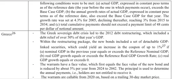
! (+! GDP (or GDP per capita) of those issuing countries rose above a certain threshold. There are other examples of GDP-linked warrants’ issuance, such as Bosnia Herzegovina and Singapore and more recently by Argentina, Greece and Ukraine. The characteristics of some of those issues are summarized in the Table 4 below.

Issuer

country Main features

Bulgaria(" . As a consequence of Bulgaria’s (external) debt crisis.

. In 1944 Bulgaria signed a Brady contract for the reduction and restructuring of its debt.

. Within the restructuring deal there was a clause for recovery of the value and payment was triggered if: (a) current GDP was equal or higher than 125% of GDP in 1993 and (b) there was a GDP increase compared to the previous year.

. If those conditions were met, the extra interest rate would be half of the GDP percentage increase (paid in the addition to the underlying plain vanilla coupon). . According to (Miyajima 2006) the source of reference data and GDP measurement

units is “ambiguous” and the corresponding term sheet is not clear in the units of measurement.

. These warrants were ‘callable’ and were inseparable from the plain vanilla bonds. Bosnia and

Herzegovina((

. In the sequence of the war in Bosnia (1992-1995) that, among other disastrous consequences, led to a significant fall in GDP. The country inherited a legacy of disadvantageous conditions from Yugoslavia, among which, (partially) a considerable high external debt.

. In 1997 an agreement on the debt restructuring was achieved and a GDP-performance bond was “settled”.

. According to (Miyajima 2006) payment on this GDP-warrants would be triggered if: (a) GDP would hit a predetermined target level and would remain at such level for two years and (b) GDP per capita would rise above US$2.80 in 1997 units, adjusted for German consumer price inflation

. Also according to the same author, this instrument suffered from poor design and low quality data.

. As the Bulgarian GLWs, were also inseparable from the plain vanilla bonds.

Singapore() . Issuance to low-income citizens of two sets of shares linking payments to GDP-growth (neither tradable nor transferable and could be exchanged only for cash with the government).

. The first share – the New Singapore Shares (NSS) – was introduced in 2011 with the purpose of helping the lower-income group during economic downturns.

. It consists of annual dividends (on outstanding balances) in the form of bonus shares with a guaranteed 3% minimum rate. An extra dividend, when applicable, corresponds to the real GDP growth rate (if positive) of the previous year.

. The second share – the Economic Restructuring Shares (ERS) – were issued with the aim of subsidizing citizens given the Goods and Services Tax increase from 3% to 5%. . Calculation of bonuses is similar to the one of NSS.

Argentina(& . Following a period of a severe economic and financial crisis, Argentina defaulted in its sovereign debt obligations by US$82 billion.

. After a period of hard negotiations with bondholders of the defaulted debt, in 2005 a debt restructuring was accepted by 76% of them, leading to a bond exchange of US$62 billion in principal.

. It included 30-year GDP-linked warrants (GDWs) that were attached, for a period of 180 days, to the new bonds.

. GLWs had no principal and, after the above-mentioned period, could act as “series of standalone, state-contingent coupons”.

. These instruments were issued in different countries and currencies.

. The GLWs would pay annually 5% of excess GDP (defined as the difference between actual real GDP and Base Case real GDP, converted to nominal pesos(*) if all the !!!!!!!!!!!!!!!!!!!!!!!!!!!!!!!!!!!!!!!!!!!!!!!!!!!!!!!!

(" _{(Pirian 2003), (Miyajima 2006).}

(( _{(Stumpf 2010), (Miyajima 2006).}

() _{(Government of Singapore - Ministry of Finance 2008), (Miyajima 2006).}

(& _{(Benford et al. 2016), (Miyajima 2006).} (*