0
A work project presented as part of the requirements for the Award of the
Masters Degree in Finance from Nova School of Business and Economics
Nominal and Inflation-Linked Government Bonds
An assessment of arbitrage opportunities in UK Gilt Market
João Pinto Teixeira Vilas-Boas, number 414
A Project carried out on the Financial Markets Area, under the supervision of:
Professor André Silva
1
Nominal and Inflation-Linked Government Bonds: An assessment of arbitrage opportunities in UK Gilt Market
Abstract: This study is an assessment of the existence of deviations of the Law of One Price in the UK sovereign debt market. UK government issues two types of debt
instruments: nominal gilts and inflation-linked (IL) gilts. Constructing a synthetic bond
comprising the IL bonds and also inflation-swaps and gilt strips I was able to build a
portfolio that pays to investor exactly the same cash-flow as nominal gilts, with the
same maturity. I found that the weighted-average mispricing throughout the period of
2006-11 is only £0,155 per £100 notional. Though, if I restrain my analysis to the
2008-09 crisis period, this amount raises to £4,5 per £100 invested. The
weighted-average mispricing can reach values of £21 per £100 notional or, if measured
in yield terms, 235 basis points. I have also found evidence that available liquidity on
the market and increases on index-linked gilts supply do play a significant role on
monthly changes of mispricing in the UK market. I concluded that, although the global
mispricing is not significant on UK gilt market, every pair of bonds in the sample
presented huge and significant arbitrage opportunities in downturn periods.
2
1.
Introduction
The basics of the Law of One price defend that if two instruments pay an investor
the same, they should be equally priced. On the sovereign debt market the theory should
also hold. As the present study suggests, that doesn’t happen in the UK gilt market. It
was found that index-linked gilts, on average, are undervalued in relation to the nominal
gilts. The mispricing1 is not always constant through time, often changing its sign. Still,
at the crisis period it reaches a huge positive magnitude. During that period, the
mispricing of a single index-linked gilt in relation to its nominal counterpart can reach
values above £28 per £100 notional. On average, the index-linked gilts reach a
mispricing maximum of 21% of the notional invested.
The methodology used on the present study is mainly based on two instruments
issued by the governments on their sovereign debt balances: nominal and
inflation-linked government bonds2 (ILB). An investor who buys an inflation-linked
bond can, by entering in an inflation swap agreement, turn his variable cash-flows into
fixed ones. Additionally, through the usage of strips, the investor is able to build a
synthetic bond that pays exactly equal cash-flows to the ones paid by nominal bonds
with same maturity. The final price of both instruments will allow an assessment of
whether or not there is mispricing (and with which sign).
Based mainly on Fleckenstein, Longstaff and Lustig (2012), the present study is of utmost importance since it aims at providing an insight on the mispricing in other
markets than in the American one. By doing so, I try to test if the American bond prices
relationship holds in markets outside America (namely in the UK) or if the TIPS
mispricing is an isolated case when studying ILBs. It also goes in line with the literature
1
Throughout this study, the term mispricing will stand for an undervaluation of the IL bonds in relation to the nominal counterparts. A negative mispricing stands for the opposite relationship.
2
3 by trying to study, in a simplistic way, what might be the factors causing mispricing in
UK market and compare them with the results for the American case.
In order to perform the aforementioned strategy, data for UK gilt market was taken
from January 2006 until the end of 2011. Although the average mispricing is positive,
presenting a value of £0,155 per £100 invested (this value goes up on the 2008-09
period for 4,5% of the notional) or 6,84 basis points, two of the five pairs selected had a
negative mispricing. The first does not include the crisis years, a period that turned out
to be the most relevant factor on the analysis of the remaining pairs. The second one,
though, was also the one presenting the higher mispricing occurrence. All of the pairs
considered presented negative mispricing clustering periods throughout the sample.
Since all bond pairs presented great mispricing levels on the crisis period, a further
analysis leaded to a comparison between the changes on mispricing with the returns of
the stock market. In fact, as it was predictable, the higher levels of mispricing were
verified on periods of weaker performance of the market.
Such times are characterized by lower investing capacity of the investors. As such,
the study tried to test if the mispricing levels are caused either by shortages of capital
available or by changes on bonds supply. Both factors turned out to be relevant, being
the returns on the stock market, the investing capacity of global hedge funds and the
supply of IL gilts significant variables for the monthly change of mispricing. The results
are aligned with previous similar studies for the American market. Still, relation
between mispricing and bonds supply is quite different. On the gilt market, supply of
nominal instruments is not significant (in contrary with what happens in the American
market) and issuing ILBs creates the opposite effect on mispricing of the American
4 The rest of this paper is organized as follows. Section 2 aims at providing a brief literature review of the related studies. Besides giving a brief description of the main
differences between nominal and ILBs, section 3 provides a description of UK markets for each of the fixed-income instruments. Section 4 describes the arbitrage strategy built in order to perform the study as well as the data used. Section 5 scrutinises the size of mispricing as well as further issues on this matter. Concluding remarks are present on
section 6.
2.
Literature Review
This study is consequent to some recent literature on the Asset Pricing Puzzle
resulting from the mispricing between the two aforementioned types of Government
debt instruments. Namely Fleckenstein, Longstaff and Lustig (2012) studied the relationship between TIPS and Treasury bonds and concluded that there was,
consistently, a great mispricing between the two types of securities. Their evidence
suggests that the nominal markets are usually overpriced when comparing with the
TIPS market.
Other important studies on this subject include an even more recent study by
Fleckenstein (2012), who performs an analysis for several other countries. The evidence on G7 countries’ markets points to the same conclusions previously mentioned
for US data and so, challenging the Asset Pricing Theory and the Law of one Price.
Both studies are not focused solely on measuring the mispricing on the bonds
market. The authors go further in the matter, analysing which factors can be on the roots
and on the persistence of the mispricing as well as its financial and economic
implications. Yet, they focus their studies mostly on the scope of the Slow-moving
5
Todd Pulvino (2007) and state that arbitrage opportunities may arise and persist in time due to some frictions, as liquidity shortages. Although basing the present study on these
papers, I have tried to hold off my analysis from the Slow-moving Capital theory, as
further considerations would have to be made on that matter.
3.
UK fixed-income Markets
This section aims at providing some insights about the fixed-income instruments
and respective markets relevant for the building of the proposed arbitrage strategy. A
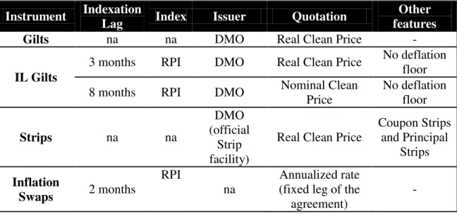
summary of each instrument features can be found on Appendix A, table 1.
The first three instruments are traded on the UK Gilt Market, responsibility of the
UK Debt Management Office (DMO). The main responsibility of this entity is the
issuance of the sovereign debt instruments, as conventional gilts and index-linked gilts
(at the end of March 2012, the latest accounted for around 22,8% of the total gilt
portfolio3).
UK Conventional Gilts
Nominal Gilts constitute the largest part of UK Government bonds portfolio. This
instrument defines an obligation between the Government and the debt-holder: the
former receives the bond price, whilst the second receives several fixed interest
payments with a specific frequency within a year4. At maturity, the debt holder receives
the last coupon and also the face value of the instrument.
UK Index-Linked Gilts
Nowadays, inflation-linked government bonds have been gaining major importance
in Europe, as their outstanding volume has been increasing since the beginning of the
last decade. This trend is observable both in Euro Area countries (with relatively recent
3
DMO - UK Government Securities: a Guide to ‘Gilts’ – Tenth Edition 2012
4
6 issuances from the French, Italian and German governments), which increased ten times
the outstanding volume since 20025, and also in non-Euro Area countries as UK and
Sweden. In Appendix A, figure 1, one might find a ranking of the main issuers of inflation-linked debt in the World as well as their respective issued notional amount.
Focusing on the UK’s case, British Government started to issue ILBs in 1981,
being one of the first issuers of such kind of debt instruments between developed
countries. The government acted in response to a great decrease in real value of nominal
debt caused by the rising inflation at the 70ies. In such way, debt was endowed with an
anti-inflationary measure that could protect its value. Moreover, those instruments
would overcome the reducing demand for sovereign instruments on inflationary periods.
Inflation-linked gilts are also characterized by a coupon rate. However, each
payment – which is made twice a year in all the existent UK government ILBs – is
adjusted for inflation. This is, coupons and the principal payment are adjusted for the
RPI index (General Index of Retail Prices), in order to account for the change in
inflation since the issuance of the bond. This adjustment is made by an indexation factor
which, further, it will be called It. It is calculated by doing the ratio between reference
RPI at payment date and the reference RPI at issuing date.
DMO’s portfolio is constituted by two different index-linked gilts. They differ on
the price calculation, in result of different indexation lags. The reference RPI to be used
in each indexation factor depends on the lagging of these bonds.
Bonds issued prior to 2005 have an 8-month lag, while all bonds issued after that
date have a 3-month lag6. Besides the difference on the computation of the indexation
factor, they also differ on the price calculation and quotation. The 8-month lag bonds
5
Danmarks Nationalbank (2011)
6
7 are quoted on nominal terms, this is, their price is adjusted for the inflation verified
since the issue of the bond. This price is obtained by multiplying the “real price”7 by the
indexation ratio. These bonds prices are often quoted above £200 since the RPI had
risen by more than 200% since 1983 (when the government started issuing
inflation-linked bonds)8. The bonds using a lagging mechanism of 3-months (also called
Canadian Style), are quoted in real terms (as it happens with the nominal gilts). There
are also differences to take into account on the cash-flow and accrued interest
calculation9.
In contrary with what happens with US TIPS, inflation-linked gilts do not have a
deflation floor. This means that if there is a deflationary effect from the issuance to the
maturity, the principal value can go below the settled par value.
UK Gilt Strips
The process of stripping a bond consists in separating each cash-flow paid by the
gilt into individual zero-coupon bonds. This means that each Strip will only pay to its
holder one cash-flow on its maturity. In example, a one year maturity bond paying a
semi-annual coupon of 2% would be strippable into 3 Strips: two paying 1 on each
semester, and other one paying 100 on the maturity. In UK the process of stripping
issued bonds was started in 1997, with the introduction of an official Strip facility.
Inflation Swaps
The most common inflation swaps are the zero-coupon (ZC) inflation swaps. This
kind of securities is considered to be the standard inflation derivative10. A ZC inflation
swap is an agreement between two parties: a buyer and a seller. They are used as
7
The term “real price” means that the price is quoted for 100 units of principal. It works as a percentage of the principal.
8
Brynjolfsson (2002)
9
Price, cash-flow and accrued interest calculations for both type of bonds are explained on DMO’s handbook Formulae for Calculating Gilt Prices from Yields
8 protection instruments against inflation risk. This kind of security only pays one
cash-flow at its maturity date. Whilst the buyer pays to the seller a fixed rate, s, this one
pays inflation indexed cash-flows (in UK case, the value of the RPI from the issuance to
the maturity date – again It) to the former. The fixed rate, s, reflects the inflation
expectations during the lifetime of the agreement. The cash-flow transaction is depicted
on figure 2.
The quotation of the ZC inflation swaps is made through the stated fixed rate. There
are quotations ranging the 1-year to 50-years maturity. As the inflation-linked bonds,
these rates do also have a lagging mechanism. The UK’s inflation swaps have a 2
months lag (and so they report to the two-months prior RPI). This may play an
important role on defining the arbitrage strategy as it will be further explained on the
next section.
4.
How to measure the Mispricing?
Strategy
Measuring a hypothetical mispricing between inflation-linked and nominal bonds,
implies that an arbitrage strategy is built11. An investor pursuing this kind of strategy
starts by taking a position on a nominal bond. This instrument pays in a semi-annual
frequency a coupon c (considering a par value of 100).
Similarly, a position on an ILB should be made. Such investment should be made
on an ILB maturing on the same date as the nominal bond, in order to compare
11
Both strategy and methodology followed the steps taken by Fleckenstein, Longstaff and Lustig (2012)
Buyer Seller
notional(1+s)t
notional(It)
Net Cash Flow to the Seller:
notional(1+s)t - notional(It)
9 cash-flows. The former pays a semi-annual coupon b. As explained in the previous
section, each coupon payment will be adjusted for inflation by a factor It, and so, the
cash-flow of each semester before maturity will be bIt (at maturity, (100+b)It).
In order to turn each variable cash-flow into a fixed one, the investor has to enter in
ZC Inflation Swap agreements – paying a fixed inflation swap rate of s. The maturity of
each agreement should match the ones of the ILB coupon payments as well as the
notional value should equal the fixed component of the ILB’s coupon, b. In a particular
date, t, the cash-flow provided by the swap agreement will be b(1+s)t – bIt. By taking
this position on the swaps for each of the ILB payments, all the cash-flows to the
investor will be non-variable12.
Finally, to eliminate the differential between the cash-flows available of the two
instruments, the investor will have to take a small position on the Strips market. That
position is equal to the difference between each nominal and inflation-linked cash-flow.
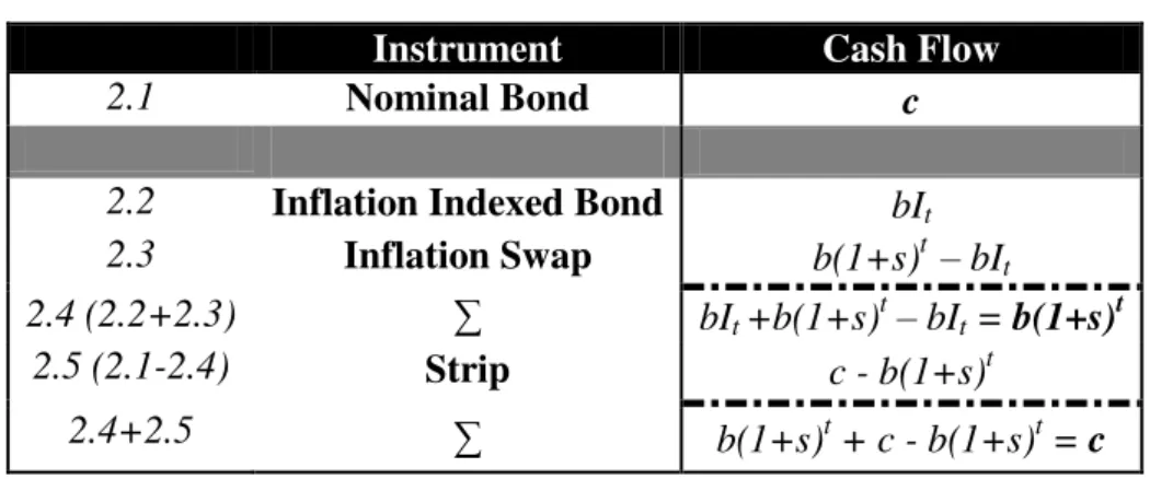
As it can be seen on table 2, and following the steps described above, at a particular date t (that can be generalized for all the payments of the securities), the final
cash-flows present a perfect match.
12
The sum of ILB cash flows and Inflation swaps considering a general case, date t, will be: bIt
+b(1+s)t– bIt = b(1+s)t
Instrument Cash Flow
2.1 Nominal Bond c
2.2 Inflation Indexed Bond bIt 2.3 Inflation Swap b(1+s)t – bIt
2.4 (2.2+2.3) ∑ bIt +b(1+s)t– bIt = b(1+s)t
2.5 (2.1-2.4) Strip c - b(1+s)t
2.4+2.5 ∑ b(1+s)t
+ c - b(1+s)t = c
10 The mispricing, then, can be measured by comparing the nominal bond price with
the price of all positions taken in the synthetic bond. In case of non-violation of the Law
of One Price equation 1 must hold.
(1) Gilt Price = IL Gilt Price + ( ∑ Strips Cash-Flowsi ) Price of Stripi13
Data and Methodology
In order to perform the aforementioned strategy, I have gathered daily prices for
UK conventional, index-linked gilts and Strips from January 3rd, 2006 to December 30th,
2011 (all the prices are adjusted for accrued interest). For the inflation swaps, daily data
was also taken but from July 1st, 2005 to the end of 2011. Although the data for all
securities is available on the Bloomberg terminal, Strips prices were taken from DMO’s
website.
The first step was to select all the possible matching pairs of bonds. The securities’
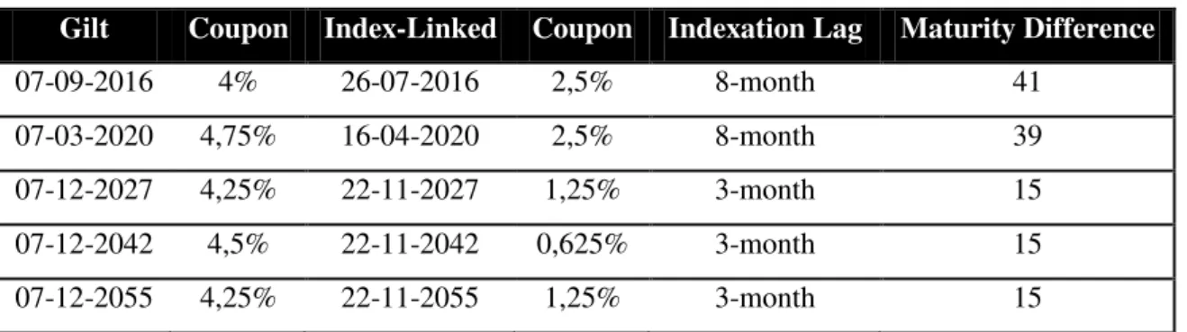
maturity gap must be the lower possible. There are any pairs with equal maturities so,
defining a two-month criterion for maturity differences, five pairs of bonds were
selected. Their main features are summarised on table 3.
Table 3: Selected pairs of conventional and index-linked bonds
Gilt Coupon Index-Linked Coupon Indexation Lag Maturity Difference
07-09-2016 4% 26-07-2016 2,5% 8-month 41
07-03-2020 4,75% 16-04-2020 2,5% 8-month 39
07-12-2027 4,25% 22-11-2027 1,25% 3-month 15
07-12-2042 4,5% 22-11-2042 0,625% 3-month 15
07-12-2055 4,25% 22-11-2055 1,25% 3-month 15
In order to start building the strategy, monthly fixed rates for the Inflation Swaps
were needed. From Bloomberg I had access to daily closing prices of inflation swaps
with maturities of 1, 2, 3, 4, 5, 6, 7, 8, 9, 10, 12, 15, 20, 25, 30, 40 and 50 years.
13
11 The monthly fixed rates can be obtained from the set of annual rates using an
interpolation method. In order to get a smooth curve the method chosen was the cubic
interpolation. The higher the interpolation degree is, the smoother the curve14. However,
having monthly rates, seasonality on inflation should be taken off the series.
Therefore, following the literature15, in order to estimate seasonality effects, a
dummy variable model should be built. I have taken monthly data for the RPI index
since January 1980 until December 2011. Given those numbers, logarithms of
moving-base index numbers were calculated in order to capture the changes in the RPI.
The last step was to use an Ordinary Least Squares regression of the logs on monthly
dummies, mi (m1=January, m2 = February, (…), m12=December ).
(2) log(RPIt/RPIt-1) = ∑ , where
(3)
A first normalization was calculated in order to get each month corrected seasonal
effect. After calculating the regression coefficients, one should subtract the average of
all the coefficients to each one of them16.
(4) ̅
Then, the seasonal adjustment factors, mi, are obtained by scaling the corrected
coefficients, turning the product of all factors equal to 1. The rationale here is that this
will guarantee that full year swaps are not influenced by seasonal patterns.
In order to take the seasonal effects from the interpolated rates, one should find the
forward rates, f, corresponding to each estimated month. Equation 5 describes the formula used for the computation.
14
Wanningen (2007)
15
Fleckenstein, Longstaff and Lustig (2012)
16
12 (5) fa-b =
17
The monthly inflation swap rates adjusted for seasonality are obtained by
multiplying all the forward rates for the seasonal adjustment factors and converting
them again into spot rates.
After calculating the monthly inflation swap rates, I was able to start building the
strategy explained on the previous subsection. However some adjustments should be
made. The first has to do with the fact that 8-months index-linked gilts are quoted in
nominal terms. In order to compute the mispricing, and because all the other prices are
on real terms, the nominal price should be divided by the respective indexation ratio in
order to get the real price.
(6) Nominal Price = Real Price
18
The second adjustment is made when entering on inflation swap agreements. Here
and as aforementioned, the differences on the lagging should be taken into account. As
the UK’s inflation swaps have a two-month lag, the rate used on a specific date of the
strategy must not be the one quoted on that day. For 8-months and 3-months
index-linked gilts, the rate to apply on the strategy should be the one quoted exactly on
the preceding sixth and first month respectively. This step is crucial in order to
overcome the differential on the lagging between the two instruments.
Finally, cash-flows should be adjusted for the maturity mismatch. The inflation
indexed synthetic bond should equal the maturity of both conventional gilts and strips.
For that purpose, I have calculated the yield to maturity of the synthetic bond
17
Cassino and Pepper (2011) state that that formula can be applied when calculating forward rates for zero-cupon inflation swaps.
18
13 comprising ILB and inflation swap agreements’ positions. This allowed me to calculate
the price of a new synthetic bond exactly matching the nominal gilt maturity19. The
remainder of the strategy is simply follow the steps described on the previous
subsection
5.
Is there any arbitrage opportunity on Gilts Market?
The main results from applying the arbitrage strategy on the Gilt market can be
observable on Figure 3. The left-hand side graph depicts the magnitude of the mispricing in British Pounds. Each bar is identified by the inflation-linked bond of the
pair. Besides the amplitude of the mispricing, observable by the range between the
minimum and the maximum mispricing per £100, the average mispricing is plotted with
the black marker. The right hand-side also shows the mispricing but measured as the
difference on the yield to maturity of the gilt and the synthetic bond (in basis points).
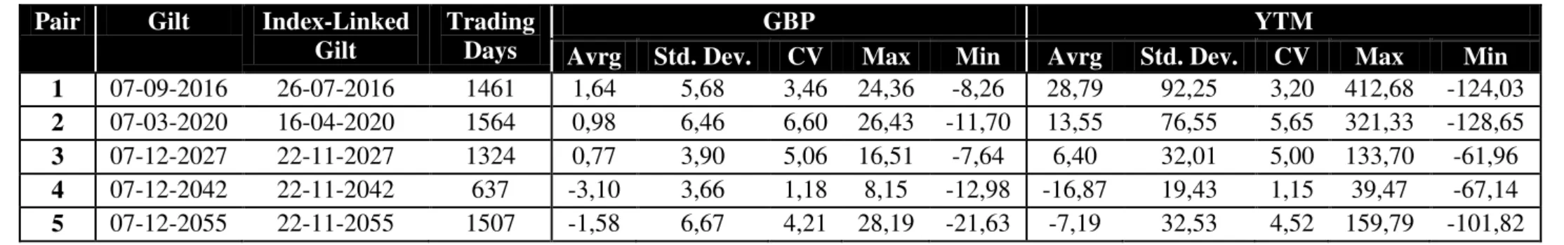
On Appendix B, table 4 summarizes the statistics for the five pairs, including the number of observations and also the standard deviation and the coefficient of variation.
19
The price computation took into account the accrued interest calculation diferences for the two types of IL Bonds
14 The results described on figure 3 and on table 4, appendix B, are not completely clear in what concerns the existence of mispricing in the UK sovereign debt market.
Three of the five pairs do show an average mispricing of the index-linked securities.
The other two have, on average, a negative mispricing. Yet, all the pairs reached a
significant mispricing value at some point of the sample period20. The longer maturity
pair, although presenting a negative mispricing average of £1,58 per £100 notional,
present the higher maximum value between all pairs included (28% of notional).
The results can be compared with the ones reached by Fleckenstein, Longstaff and Lustig (2012) for the United States21. By doing so, one might conclude that evidence on US markets for mispricing is much more conclusive than in the UK market.
In all 29 pairs included on their study, the authors report a positive mispricing of the
inflation-indexed bonds in relation to the nominal ones. Moreover, only ten do present
cases of overpricing of the Treasury nominal bonds over all sample period. On average,
the mispricing on US market is constantly positive, fact that does not occur in any of the
UK pairs that present times of negative mispricing clustering, as it can be seen on
Appendix C, figure 4.
Comparing also the five pairs included in the sample, one might not conclude that
the mispricing level varies either with maturity or with the lagging mechanism. Even
though longer maturities and 3-month index-linked gilts are the ones presenting lower
mispricing levels, the 2055 maturity pair, as aforementioned, is the one that presents a
higher mispricing occurrence.
20
Issues on this matter will be discussed in detail further in this study 21
15 Following the literature22, in order to measure the occurrence or not of mispricing
in the gilt market, for each trading day, I have computed a weighted average of all the
pairs that were available on that date. The daily mispricing is weighted by each
inflation-linked gilt notional amount (in total) issued. The average mispricing of all
securities is only £0,155 per £100 notional. However, analysing the respective statistics,
the mispricing reaches a level of around £21 per £100 notional (at the end of 2008),
which is a huge value when comparing with the maximum mispricing verified on US
and computed on the study previously mentioned (9,6% of the notional).
Moreover, a deeper analysis throughout the sample leads to the conclusion that the
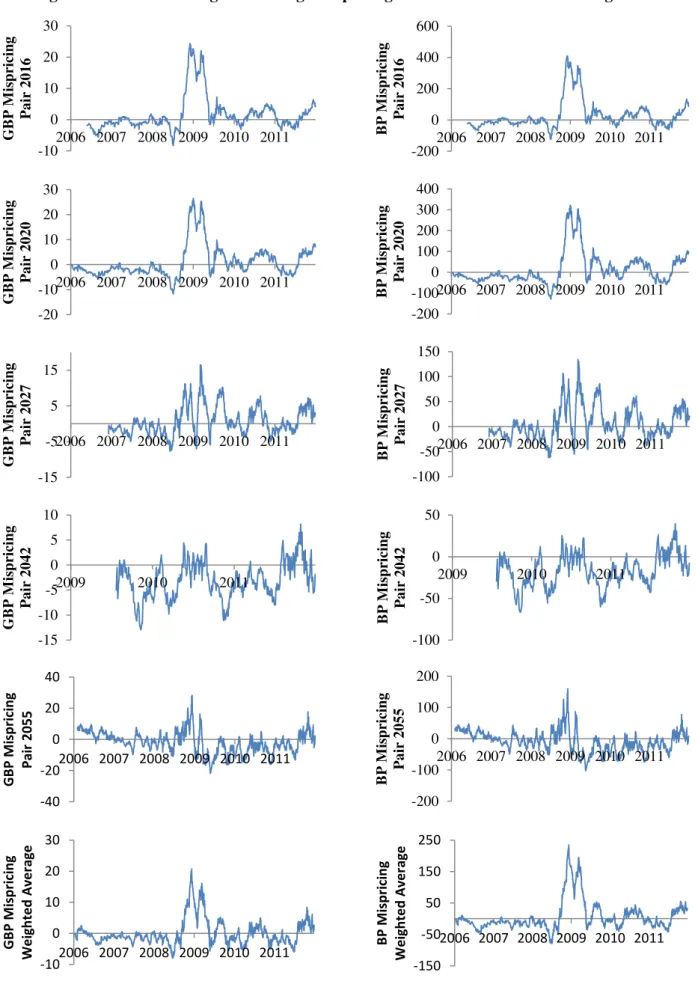
2008-2009 crisis had a great impact on the gilt market mispricing. The mispricing
values were plotted on the graphs presented in appendix C, figure 4. The ten graphs on the top depict the mispricing in all five bond pairs (in British pounds and in basis
points), while the two in the bottom shows the weighted average mispricing throughout
the sample period.
As suggested on all graphs, in the period of the crisis, after September 2008 and
until middle of 2009, the mispricing magnitude is huge. Comparing with the remaining
sample period, where the amplitude of mispricing is very unstable – varying from
periods with negative mispricing to others with a positive one -, the behaviour of the
series in that period stands out. In fact, restraining the sample period to the period from
September 2008 until December 2009, the weighted-average mispricing jumps to over
£4,5 per £100 notional.
The (non)existence of a deflation floor for the index-linked bonds does play a role
on the mispricing. In case of inflation-linked gilts, as already mentioned, they do not
22
16 have a deflation floor. In other words, at the maturity, if a deflation is verified the
principal value of the bond is adjusted downwards. If IL gilts were endowed of such
feature, the mispricing amplitude would be smaller. As a remark, transaction costs even
though not considered in this study, would not have a great impact on gilts mispricing
(mainly in the crisis period)23.
The observable impact of downturns on mispricing turns out to be one plausible
explanation for the lower values of mispricing verified on the pair maturing on 2042.
The index-linked gilt was only issued on July 2009 and so the most relevant period for
the other pairs’ mispricing had to be excluded from the analysis.
So, it is now interesting to investigate how the mispricing behaved with the stock
market returns. In order to do so, changes on monthly mispricing measured in basis
points were calculated for the weighted-average mispricing series. On Appendix D, figure 5, those fluctuations were plotted against the returns on the London Stock Exchange Index (FTSE 100).
Although not completely clear, the graph shows a negative relation between the two
variables, confirmed by a correlation coefficient of -0,23. Such relationship is much
more obvious on the crisis period then in other periods in which both variables move
alongside with each other. It is so plausible to argue, that such relation can appear due to
other factors than the performance of the stock market itself.
Further issues on Gilt Market Mispricing
Following the literature, some factors to analyse the mispricing in the Gilt market
were considered. Kilponen, Laakkonen and Vilmunen (2012), study the impact of Central Bank policies on the sovereign debt yields. In order to do so, the authors
23
17 considered some variables that might influence bond yields. Some of those factors were
considered also as potential drivers for the mispricing on the US markets by
Fleckenstein, Longstaff and Lustig (2012).
In order to complement the previous analysis of the influence of stock markets
performance24 on mispricing in the Gilt market, a market risk perception measure was
considered. The referred authors include on their sample a global uncertainty feeling,
which is often measured by the implied volatility index for S&P500 (VIX). Furthermore,
as argued by Nagel (2011) and Fleckenstein (2012), implied volatility is also a liquidity provision proxy. Periods of downturns are also periods when risk perception is higher
and liquidity is restrained. This might influence the occurrence of mispricing.
On Appendix D, it is plotted on figure 6 the monthly variation in basis points of the weighted-average mispricing against monthly data for VIX. Additionally, as values
of VIX of 20% might indicate less worrying times on the market, while an index over
30% signals high uncertainty25, a green and a red dotted line were plotted on the graph
for those values respectively. As it might be expectable, the mispricing variation peaks
coincide with the times when implied volatility is higher. Periods of high perception of
risk (observable by the occurrences above the plotted lines) are the ones where the
series denote a more similar behaviour. Indeed, the global market perception of risk,
and the mispricing on Gilt markets, present a correlation of 0,28. The evidence seems to
confirm that high turbulence times have impact on the mispricing.
In order to conclude this analysis a regression was estimated in order to try to test
which factors are responsible for the mispricing. This regression was based on the
24
Mitchell, Pedersen and Pulvino (2007)
25
18 literature referred above and sticks to two main drivers for mispricing: the liquidity
available for investors and the supply of bonds.
Complementarily, Brunnermeier and Pedersen (2009) discuss market liquidity in the scope of its co-movement with the market and its relation with volatility. As such,
the two already analysed variables, stock returns and the returns on the VIX index, were
considered as measures of liquidity. Basing on Fleckenstein, Longstaff and Lustig (2012), the authors also include on their model the Global Hedge Fund Index as a proxy for the liquidity available for investors, globally. As the authors argue, the investing
capacity of hedge funds does seem to influence asset pricing. This index is available on
the Bloomberg terminal with the ticker HFRXGL, and the monthly return of the index
was considered as explanatory variable.
The supply factor was considered following the same literature. The authors
concluded that for the US market, both supply of treasury and TIPS influence
negatively the mispricing. Thus it is interesting to test whether or not such relationship
verifies on the UK market. For this purpose, month-to-month changes on supply of
either nominal or index-linked bonds were considered. Both series were built based on
issue data taken from the DMO’s website.
The dependent variable considered was the monthly change on basis points
mispricing (the weighted-average series for all sample pairs). The aforementioned
variables are identified, respectively, by the following names: FTSE; VIX; HF;
Supply_nominal and Supply_IL. The first three variables are in percentage, whilst the
latest two are on million £. The model considered is described by equation 7.
19 The output of the regression is presented on table 5, appendix D and it allows us to take some interesting conclusions. The first factor considered, available liquidity,
do present significant results. Both performance of the stock market and the variation on
the hedge-funds capital are statistically significant for a 99% confidence level. A
negative coefficient on both variables was achieved. In what concerns the performance
of the market, this result is aligned with the previous analysis. A decrease on stock
returns leads to an augmenting of the mispricing. The evidence that in periods of
troubled waters the arbitrage opportunities on the gilt market arise is so confirmed. A
shortening of hedge funds investing capacity should also cause an increasing
mispricing. Such statement is confirmed by the negative sign of the regressed variable.
The returns of implied volatility index, though, are not significant for any reasonable
confidence level.
The results for bonds supply are interesting, since they deviate from the ones
presented for the US case, studied on the papers previously referred. On the UK market
the supply of nominal bonds doesn’t seem to be significant. Such variable would only
be significant for confidence levels of around 85% (before the usual corrections for
heteroskedasticity, the variable was significant). Yet, it presents a negative sign which
comes in hand with the results presented by the authors for the US case. On contrary,
the supply of inflation-linked gilts is significant for a 2,5% level. Though, its sign is the
opposite of the US similar variable. The model provides evidence that an increase of the
amount of ILB available has a positive impact on mispricing and so, the composition of
the Government debt structure influences the mispricing. An increase of the amount of
IL gilts issued widens the mispricing, which means that it drives down their prices in
20 The model, having global significance, confirms that both supply of bonds and
liquidity available on the market do influence the mispricing on the market. Such results
are, in general, aligned with the three studies mentioned on this section of the study.
6.
Conclusion
This study provides an assessment to arbitrage opportunities in the UK sovereign
debt market. The theory predicts that if two assets generate the same cash-flows to an
investor, they should be equally priced. However, in various markets this principle is
not verified and, as proven, the Gilt Market is one of them. The present work project
estimates that, on average, the inflation-linked bonds are undervalued by a value of
£0,155 per 100£ notional in relation to their nominal counterparts.
Although the presented value is not as high as the one reached by related literature
for the US case, one should not rely solely on this value. The magnitude of mispricing
on the gilt market is much more significant in the 2008-09 crisis. Indeed, the weighted
average mispricing on those years was £4,5 per £100 notional and had as maximum
mispricing a value of 21% of the notional. These occurrences are very significant and
above the ones estimated for the US. Still, it is shown that, on the UK, mispricing often
changes the sign of its values. Negative mispricing is, generally, clustered on time.
Finally, these findings lead the mispricing analysis to the scope of market
performance. As expected, in times of high turbulence of the markets the mispricing
increases. Also, it is on those times that there is a shortening of liquidity provision for
investors. As such, evidence was found that this factor do play a role on the changes of
mispricing. The returns on the market and the investing capacity of global hedge funds
have a significant influence on the mispricing. Additionally, the increase on the supply
21
7.
References
Belgrade, Nabyl, and Eric Benhamou, 2004. “Smart Modeling of the Inflation Market: Taking into Account Seasonality.” Risk Magazine, Inflation Risk, July 2004 Supplement
Brunnermeier, Markus, and Lasse H. Pederson, 2009, “Market Liquidity and
Funding Liquidity.” The Review of Financial Studies, 22: 2201-2238
Brynjolfsson, John B.,2002. “Chapter 8: Inflation Indexed Bonds.” In The Handbook
of financial instruments, ed. Frank J. Fabozzi, 203-215. Hoboken, New Jersey: John
Wiley & Sons, Inc.
Danmarks Nationalbank, 2011. “Danish Government Borrowing and Debt.”
http://www.nationalbanken.dk/C1256BE900406EF3/sysOakFil/SLOG_2011_uk_web/$ File/SLOG_2011_uk_web.pdf
Fleckenstein, Matthias, 2012. “The Inflation-Indexed Bond Puzzle.” Working Paper, UCLA Anderson School
Fleckenstein, Matthias, Francis A. Longstaff, and Hanno Lustig, 2012. “Why does the Treasury Issue Tips? The TIPS-Treasury Bond Puzzle.” The Journal of Finance, Forthcoming
Kerkhof, Jeroen, 2005. “Inflation Derivatives Explained. Markets, Products and Pricing”, Fixed Income Quantitative Research, Lehman Brothers:1-80
Kilponen, Juha, Helinä Laakkonen, and Jouko Vilmunen, 2012. “Sovereign risk,
European crisis resolution policies and bond yields.” Bank of Finland Research
Discussion Papers, 22
Mitchell, Mark, Lasse H. Pedersen, and Todd Pulvino, 2007. “Slow Moving
Capital.” American Economic Review, Papers and Proceedings, 97: 215-220
Nagel, Stefan,2012. “Evaporating Liquidity.” TheReview of Financial Studies , 25 (7): 2005-2039
United Kingdom Debt Management Office, 2005. “Formulae for Calculating Gilt
Prices from Yields.” 3rd
edition
http://www.dmo.gov.uk/documentview.aspx?docname=/giltsmarket/formulae/yldeqns.p df&page=Gilts/Formulae
United Kingdom Debt Management Office, 2012. “UK Government Securities: a Guide to ‘Gilts’.” 10th edition
http://www.dmo.gov.uk/documentview.aspx?docname=publications/investorsguides/mb 13062012.pdf&page=investor_guide/Guide
Wanningan, C. F. A. R, 2007. “Inflation Derivatives.” Graduation Thesis Financial Engineering and Management University of Twente
Wei, Ong Kang, 2012. “UVXY: How One Can Profit From This VIX ETF”,
22 Appendix A
Instrument Indexation
Lag Index Issuer Quotation
Other features
Gilts na na DMO Real Clean Price -
IL Gilts
3 months RPI DMO Real Clean Price No deflation floor
8 months RPI DMO Nominal Clean Price
No deflation floor
Strips na na
DMO (official
Strip facility)
Real Clean Price
Coupon Strips and Principal
Strips
Inflation
Swaps 2 months
RPI
na
Annualized rate (fixed leg of the
agreement) - 10 6 9 3 7 4 5 8 2 1 0 100 200 300 400 500 600 700 800 900 Am o un t Is sued (bil lio n $ )
Figure 1 - Main Issuers of Index-Linked Government Bonds in the World (ranked) and Amount Issued (Billion $)
Source: UK Standard Life Investments and Bloomberg (values for January 2013)
Table 1 – Summarized features of the britisih fixed-income instruments considered
23
Appendix B
Table 4 – Mispricing summarized statistics: Considered pairs and respective observations. The middle panel summarizes the main statistics (average, standard deviation, coefficient of variation, maximum and minimum) in terms of Great Britain Pounds. The right panel
provides the same statistics, now for the mispricing measured in basis points.
Pair Gilt Index-Linked
Gilt
Trading Days
GBP YTM
Avrg Std. Dev. CV Max Min Avrg Std. Dev. CV Max Min
1 07-09-2016 26-07-2016 1461 1,64 5,68 3,46 24,36 -8,26 28,79 92,25 3,20 412,68 -124,03
2 07-03-2020 16-04-2020 1564 0,98 6,46 6,60 26,43 -11,70 13,55 76,55 5,65 321,33 -128,65
3 07-12-2027 22-11-2027 1324 0,77 3,90 5,06 16,51 -7,64 6,40 32,01 5,00 133,70 -61,96
4 07-12-2042 22-11-2042 637 -3,10 3,66 1,18 8,15 -12,98 -16,87 19,43 1,15 39,47 -67,14
24 -10 0 10 20 30
2006 2007 2008 2009 2010 2011
G B P M is pricing P a ir 2 0 1 6 -200 0 200 400 600
2006 2007 2008 2009 2010 2011
B P M is pricing P a ir 2 0 1 6 -20 -10 0 10 20 30
2006 2007 2008 2009 2010 2011
G B P M is pricing P a ir 2 0 2 0 -200 -100 0 100 200 300 400
2006 2007 2008 2009 2010 2011
B P M is pricing P a ir 2 0 2 0 -15 -5 5 15
2006 2007 2008 2009 2010 2011
G B P M is pricing P a ir 2 0 2 7 -100 -50 0 50 100 150
2006 2007 2008 2009 2010 2011
B P M is pricing P a ir 2 0 2 7 -15 -10 -5 0 5 10
2009 2010 2011
G B P M is pricing P a ir 2 0 4 2 -100 -50 0 50
2009 2010 2011
B P M is pricing P a ir 2 0 4 2 -40 -20 0 20 40
2006 2007 2008 2009 2010 2011
GB P M isp ri ci n g Pai r 2055 -200 -100 0 100 200
2006 2007 2008 2009 2010 2011
B P M is pricing P a ir 2 0 5 5 -10 0 10 20 30
2006 2007 2008 2009 2010 2011
GB P M isp ri ci n g Wei g h te d A v e rag e -150 -50 50 150 250
2006 2007 2008 2009 2010 2011
B P M isp ri ci n g Wei g h te d A v e rag e
Appendix C
25 0% 10% 20% 30% 40% 50% 60% 70% -100 -80 -60 -40 -20 0 20 40 60 80 100
2006 2007 2008 2009 2010 2011
VIX Ch an g e s o n M isp ri ci n g ( B asi s Point s) Mispricing VIX
Appendix D
Dependent Variable Month-to-month changes on basis points mispricing
Independent Variables Coefficient t-Statistic P-value
C 0,777 0,17 0,87
FTSE -1,986 -3,194 0,002
HF -5,406 -2,88 0,005
VIX -5,759 -0,467 0,64
Supply_nominal -0,0008 -1,438 0,155
Supply_IL 0,003 2,308 0,024
R2 0,42
F-stat (prob) 0
-20% -15% -10% -5% 0% 5% 10% 15% -100 -80 -60 -40 -20 0 20 40 60 80 100
2006 2007 2008 2009 2010 2011 Ret
urns Cha ng es o n M is pricing ( ba sis P o ints) Mispricing Returns
Table 5 – Regression output: Regression of month-to-month changes on mispricing (BP) on FTSE returns, Hedge Funds investing capacity (asset balances), VIX, and supply of Nominal gilts and IL gilts
Figure 6 – Changes on mispricing against VIX level: Below the green dotted line markets are not very volatile while above the red dotted line, markets face high turbulence