Social Accounting Matrices for Portugal in 1998-99. Modelling the effects of changes in government receipts and expenditure.
Susana Maria G. Santos
Institute of Economics and Business Administration Department of Economics
Technical University of Lisbon
Rua Miguel Lupi, 20, 1200-781 Lisboa, Portugal, E-mail: ss@iseg.utl.pt.
ABSTRACT
Aggregated Social Accounting Matrices (SAMs) will be built for the Portuguese economy in 1998 and 1999, based on the country’s national accounts statistics. The SAMs will be shown as a working instrument for quantifying the flows in the economic circuit and for simulating the effects resulting from changes in such flows.
The economic flows associated with the government subsectors will be emphasised, whilst accounting multipliers will be calculated to facilitate the study of the effects resulting from changes in the government’s expenditure and receipts, which will also be subjected to a test on their veracity.
KEYWORDS: Social Accounting Matrix; Economic Planning; Economic Policy;
Macroeconomic Modelling.
Acknowledgements: I would particularly like to thank Professor Ferreira do Amaral (Higher Institute of Economics and Business Administration) for the encouragement that he gave me and for the comments that he made on the earlier drafts of this paper. I must stress, however, that any errors or omissions in this text are entirely my own responsibility.
CONTENTS
1. Introduction ... 1
2. The Portuguese SAMs structure ... 2
3. SAM modelling 3.1. Methodology ... 11
3.2. Evaluation with changes in government subsector receipts... 15
3.3. Evaluation with changes in government subsector expenditure ... 23
3.4. Results at the level of government subsector balances ... 32
4. Summary and conclusions ... 37
References ... 40
1. Introduction
The Social Accounting Matrix, usually known as SAM, is the working instrument used in this paper to study the effects of changes in the receipts and expenditure of the different Portuguese government subsectors on the economy as a whole, as well as on the government’s budget balance in 1998.
Compiled from the Portuguese System of National Accounts (SNA), the SAMs constructed for the Portuguese economy in 1998 and 1999 can be seen as the matrix representation of government receipts and expenditure, showing the entire circular flow of income. This particular method of accounting for economic activity dates back to a number of different sources, starting with F. Quesnay’s “tableau économique” (18th century). Sir Richard Stone pioneered the development of the SAM framework with his 1954 article “Input-Output and the Social Accounts,” working on it for over roughly four decades. The general shape of an SAM framework was first described by Pyatt and Thorbecke (1976). Afterwards Pyatt and Roe (1977) published a book giving a detailed description of the example of Sri Lanka. Since then, SAMs have been applied in a wide variety of (developed and developing) countries and regions, and with a wide variety of different goals. SAMs have been used to study income distribution and redistribution (e.g. Pyatt & Roe, 1977 and Keuning, 1996), growth strategies in developing economies (e.g. Pyatt & Round, 1985a and Robinson, 1986), decomposition of activity multipliers that shed light on the circuits comprising the circular flow of income (e.g. Stone, 1981 and Pyatt & Round, 1985), as well as a combination of social, technological/environmental and economic issues (e.g. Resosudarmo & Thorbecke, 1996, Khan, 1997, Duchin1, 1998 and Alarcón &
others, 2000).
In Portugal studies have been undertaken using SAMs for 1974 (Norton & others, 1986), 1977 (Dionizio, 1983), from 1986 to 1997 (Santos, 1999, 2001 and 2003) and now for 1998 and 1999, this time with a methodological novelty (SAM modelling with transposed SAMs), a test on the veracity of the results and an
1 Her very elucidating paper entitled “Global Environmental Degradation in the 21st Century: A
Challenge for Output Economics”, presented at the 14th International Conference on
Input-Output Techniques (Montreal - Canada, October 2002), stresses the importance of the SAM
analysis of government flows, which we have never seen treated before in an SAM framework.
As will be seen in section 2, square matrices will be used, in which each transaction is recorded only once in a cell of its own – it is conventionally agreed that the entries made in rows represent incomes or receipts, whilst the entries made in columns represent outlays or expenditures. These figures will include both production and institutional accounts, which are subdivided into yet other accounts, defined in accordance with the goal of the study, as specified in the first paragraph. Thus, the constructed SAMs consist of a set of interrelated subsystems that, on the one hand, give an analytical picture of the Portuguese economy in 1998 and 1999 and, on the other hand, as will be seen in section 3, serve as an instrument for assessing the effects of changes on government expenditure and receipts (injections and leakages in the system), which might be the result of policy measures. Section 4 ends the paper with a summary, largely of section 3, and some concluding remarks.
2. The Portuguese SAMs structure
The SAMs used here were constructed with the aim of studying the effects of changes in the Portuguese government’s expenditure and receipts. Other influences affecting their construction were the available data and previous experience in the construction of SAMs (Santos, 1999, 2001 and 2003), basically inspired by the works of Graham Pyatt and his associates (Pyatt, 1988 and 1991; Pyatt & Roe, 1977; Pyatt & Round, 1985).
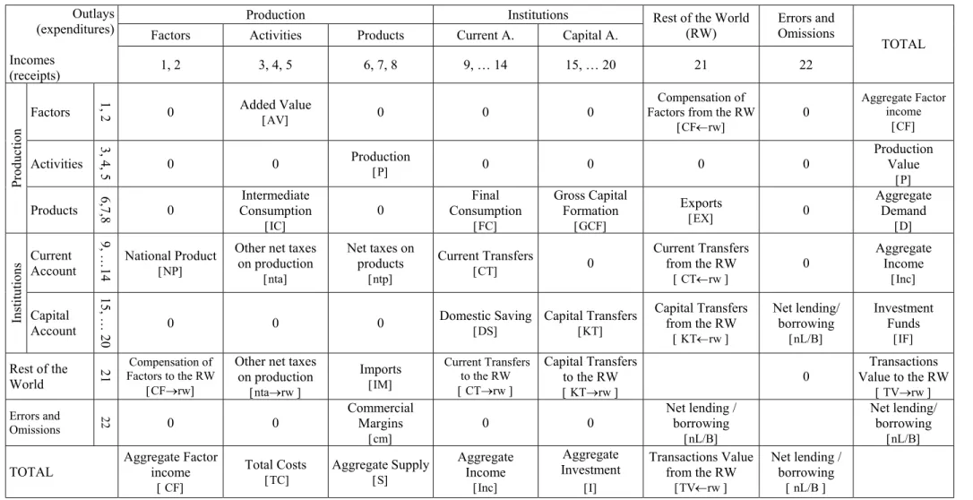
Our concern was to adopt a mutually exclusive and, to some extent, exhaustive classification, so that in the disaggregation of the Portuguese SAM accounts we have: production, divided into factors of production, activities and products; and institutions, divided into current and capital accounts2. Besides the rest of the world account, an “errors and omissions” account was also considered, which assumes values that are perfectly justified by the national accounting system. We therefore respected, on the one hand, the functional criterion (describing the production processes and pointing out the existing
technical-economic relationships between the various productive units) and, on the other hand, the institutional criterion (describing distribution, accumulation and financing activities and showing the relationships involved in economic behaviour). The criterion used for ordering the accounts was the one that underlies the “generic Portuguese SAM”, presented in Table 1.
2 In previous works, a financial account was also included. In this case, however, it was not
Table 1. Generic Portuguese SAM
Production Institutions Factors Activities Products Current A. Capital A.
Rest of the World
(RW) Errors and Omissions Outlays
(expenditures) Incomes
(receipts) 1, 2 3, 4, 5 6, 7, 8 9, … 14 15, … 20 21 22
TOTAL
Factors 1, 2 0 Added Value [AV] 0 0 0 Factors from the RW Compensation of
[CF←rw] 0 Aggregate Factor income [CF] Activities 3, 4, 5
0 0 Production [P] 0 0 0 0 Production Value
[P] Product ion Products 6,7,8 0 Consumption Intermediate [IC] 0 Final Consumption [FC] Gross Capital Formation [GCF] Exports [EX] 0 Aggregate Demand [D] Current Account 9, …14 National Product [NP]
Other net taxes on production [nta] Net taxes on products [ntp] Current Transfers [CT] 0 Current Transfers from the RW [ CT←rw ] 0 Aggregate Income [Inc] In stitu tio ns Capital Account 15, … 20
0 0 0 Domestic Saving [DS] Capital Transfers [KT] Capital Transfers from the RW [ KT←rw ] Net lending/ borrowing [nL/B] Investment Funds [IF] Rest of the World 21 Compensation of Factors to the RW [CF→rw]
Other net taxes on production [nta→rw ] Imports [IM] Current Transfers to the RW [ CT→rw ] Capital Transfers to the RW [ KT→rw ] 0 Transactions Value to the RW [ TV→rw ] Errors and Omissions 22 0 0 Commercial Margins [cm] 0 0 Net lending / borrowing [nL/B] Net lending/ borrowing [nL/B] TOTAL Aggregate Factor income
[ CF] Total Costs [TC] Aggregate Supply [S] Aggregate Income [Inc] Aggregate Investment [I] Transactions Value from the RW [TV←rw ] Net lending / borrowing [ nL/B ]
Being a numerical representation of the cycle of production – income – expenditure, the SAM “incorporates all major transactions within a socio-economic system” (Thorbecke, 2001), as can be seen in Outline 1, where, following the flows of money, the connections that can be established between the various Portuguese SAM accounts are represented.
Outline 1: Flows of money between the generic Portuguese SAM accounts
DOMESTIC ECONOMY
Notes:
(a) Gross Added Value at factor cost.
(b) Includes net taxes on products that are receipts from European Union institutions. (c) Current transfers to the rest of the world include direct purchases abroad by residents. (d) Includes direct purchases in the domestic market by non-residents.
See Table 1 for the meaning of the flows.
This outline “makes it clear that, within the macro-economy, there is a circular flow process and that what happens at one point on the circuit will have
DS Production Activities (accounts 3, 4, 5) Products (accounts 6, 7, 8) Factors of Production (accounts 1, 2) P Current Account (accounts 9,10,11,12,13,14) Capital Account (accounts 15,16,17,18,19,20)
REST OF THE WORLD (account 21) IM (b) Institutions KT↔ rw CF ↔ rw NP AV(a) nta IC ntp GCF EX (d) FC nta →rw KT CT CT↔ rw (c) nL/B
implications for experience at other junctures. This observation translates into the notion that, at some point, there is a need for being equally concerned with all the different aspects of technology and behaviour that together describe the circular flow and the connections (or lack thereof) that characterise an economy” (Pyatt, 1991a).
The SAM therefore offers a more or less disaggregated view of value flows, detailing the direct linkages between accounts, but also pointing out the scope of the underlying indirect interactions. For instance, inflows from exogenous accounts that stimulate the level of activity of a production sector, will also induce additional factor income that, once distributed among households, will be used to finance new final demand for producer goods and services (Roland-Holst & Sancho, 1995).
As is shown by the numbers of the accounts, further disaggregation was undertaken of the framework described above, always in keeping with the National Accounts Nomenclature. So, in the constructed matrices, Tables 2 and 3 (see the description of their cell contents in the annex), the factors of production were disaggregated into labour and capital and the activities and products accounts into primary, secondary and tertiary groups3. On the other hand, the current and capital accounts of institutions were divided into households, enterprises (non-financial corporations), central and local government and social security funds (which constitute the general government), and other institutions (financial corporations and non-profit institutions serving households).
Because particular attention was being given to the general government flows, advantage was taken of a crucial feature of the SAM, i.e. the wide range of possibilities that it offers for expanding or condensing it in accordance with specific circumstances and needs (ISWG, 1993, paragraph 20.6), without, however, losing sight of the consistency of the whole system.
3 The primary group includes agriculture, forestry and fishing (activities/products 01 to 05 of the
National Accounts System). The secondary group includes industry, which in turn includes energy and construction (activities/products 10 to 45 of the National Accounts System). The tertiary group includes the rest of the economy (activities/products 50 to 95 of the National Accounts System).
3. SAM Modelling
3.1. Methodology
An analysis will be made firstly of the demand-driven economy , to evaluate changes in government receipts, and then of the supply-driven economy , to evaluate changes in government expenditures. That is to say, the analysis will begin firstly in the traditional way, with receipts in rows and expenditures in columns, and then the SAM will be transposed, with expenditures in rows and receipts in columns (transposition shown by words in brackets in the
following exposition).
As described below, the base methodology of the multipliers will be used, in keeping with the work of G. Pyatt & A. Roe (1977) and G. Pyatt & J. Round (1985), which represents the basis of what has so far been done in this area.
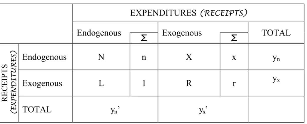
Table 4. SAM in endogenous and exogenous accounts
EXPENDITURES (RECEIPTS)
Endogenous
Σ
ExogenousΣ
TOTALEndogenous N n X x yn
Exogenous L l R r yx
RECEIPTS
(EXPENDITURES) TOTAL yn ’ yx’
Where:
N = matrix of transactions between endogenous accounts
n = vector of the row sum of N
X = matrix of the transactions between exogenous and endogenous accounts [injections from first into second/(leakages from second into first)]
x = vector of the row sum of X
L = matrix of the transactions between endogenous and exogenous accounts [leakages from first into second/(injections from second into first) ]
l = vector of the row sum of L
r = vector of the row sum of R
yn = vector (column) of the receipts (expenditures) of the endogenous accounts
yn’ = ” (row) of the expenditures (receipts) ” ” ” ”
ŷn = matrix (diagonal) of the receipts (expenditures) ” ” ” ”
(ŷn-1: inverse)
yx = vector (column) of the receipts (expenditures) of the exogenous accounts
yx’ = ” (row) of the expenditures (receipts) ” ” ” ”
From Table 4, it can be written that
yn = n + x (1)
yx = l + r (2)
It can also be seen that, in aggregate terms, total injections from the exogenous into the endogenous accounts (leakages from endogenous into
exogenous accounts), i.e. the column sum of “x”, are equal to total leakages
from the endogenous into the exogenous accounts (injections from exogenous into endogenous accounts), i.e. considering i’ to be the unitary vector (row), the column sum of “1” is: x * i’ = l * i’. (3)
In other words, the amount that the endogenous accounts receive (spend) is equal to the amount that they spend (receive) – using the words of Pyatt (1988): “a SAM is a simple and efficient way of representing the fundamental law of economics: for every income there is a corresponding outlay or expenditure”.
The accounting multipliers4, which will allow for further analysis, can now be deduced.
In the previous structure, if the entries in the N matrix were divided by the corresponding total expenditures (receipts), a corresponding matrix (squared) can be defined of the average expenditure (receipt) propensities of the endogenous accounts within the endogenous accounts or of the use of resources within those accounts. Calling this matrix An, it can be written that
4 In this type of approach, fixed price multipliers can also be used. They will not be mentioned.
An = N*ŷn -1 (4)
N = An* ŷn (5)
Considering equation (1), yn = An*yn + x (6)
Therefore, yn = (I-An)-1* x = Ma * x. (7)
We thus have the equation that gives the total receipts (expenditures) of the endogenous accounts (yn), by multiplying the injections (leakages) “x” by the matrix of the accounting multipliers: Ma = (I-An)-1. (8)
On the other hand, if the entries in the L matrix are divided by the corresponding total expenditures (receipts), a corresponding matrix (usually non squared) can be defined of the average expenditure (receipt) propensities of the endogenous accounts in (from) the exogenous accounts or of the use of resources from the endogenous (exogenous) accounts into the exogenous (endogenous) accounts. Calling this matrix Al, it can be written that Al = L*ŷn-1 (9)
L = Al* ŷn (10)
Considering equation (2), yx = Al*yn + r (11)
Thus, l = Al * yn = Al * (I-An)-1* x = Al * Ma * x. (12)
So, with the accounting multipliers, the impact of changes in receipts (expenses) is analysed at the moment, assuming that the structure of expenditures (receipts) in the economy does not change. This type of methodology allows for a static analysis to be made, assuming that there is excess capacity, prices remain constant and the production technology and resource endowment are given. If we consider the An matrix and two other ones with the same size (Bn - with the diagonal of An, whilst all the other elements are null - and Cn - with a null diagonal, but with all the other elements of An), it can be written that An = Bn + Cn. (13)
Thus, from equation (6): yn = Bn * yn +Cn * yn + x = [I – (I - Bn)-1 *Cn]-1 * (I - Bn)-1 * x 5. (14)
5 y
n = An*yn + x = Bn*yn + Cn*yn + x ⇔ yn - Bn*yn = Cn*yn + x ⇔ yn = (I-Bn)-1* Cn * yn + (I-Bn)-1 *x
⇔ yn - (I-Bn)-1 * Cn * yn = (I-Bn)-1 *x ⇔ yn * [I - (I-Bn)-1 * Cn] = (I-Bn)-1 * x ⇔ yn = [I - (I-Bn)-1 * Cn]-1 * (I-Bn)-1 * x.
Therefore: Ma = [I – (I - Bn)-1 *Cn]-1 * (I - Bn)-1 = M3*M2*M1. (15)
The accounting multiplier matrix is thus decomposed into multiplicative components, each of which relates to a particular kind of connection in the system as a whole (Stone, 1985)6.
- The intragroup or direct effects matrix, which represents the effects of the initial exogenous injection (endogenous leakage) within the groups of accounts in (from) which it had originally entered (left), that is,
M1 = (I - Bn)-1. (16)
- The intergroup or indirect effects matrix, which represents the effects of the exogenous injection (endogenous leakage) within the groups of accounts, after its repercussions have completed a tour through all the groups and returned to the one which it had originally entered (left), that is, if we consider “t” to be the number of groups of accounts,
M2 = {I - [(I - Bn)-1 *Cn ]t}-1. (17)
- The extragroup or cross effects matrix, which represents the effects of the exogenous injection (endogenous leakage), when it has completed a tour outside its original group without returning to it, in other words when it moves around the whole system and ends up in one of the other groups, that is, if we consider “t” to be the number of groups of accounts,
M3 = {I + [(I - Bn)-1 *Cn ] + [(I - Bn)-1 *Cn ]2 + … + [(I - Bn)-1 *Cn ]t-1} (18)
The decomposition of the accounting multipliers matrix can also be undertaken in an additive manner, as follows:
Ma = I + (M1 - I) + (M2 - I) * M1 + (M3 - I) * M2* M1. (19)
Where I represents the initial injection (leakage) and the remaining components the additional effects associated, respectively, with the three components described above (M1, M2 and M3).
The main aim of the present paper is to study the effects of changes in government receipts (injections) and expenditures (leakages), which led the “current” and the “capital” accounts of “central and local government and social security funds”, as well as the “errors and omissions” accounts, to be considered
6 For a detailed deduction and explanation of these components, see, for instance, Stone, 1985;
as endogenous, beyond the “production” accounts. As a result of this, the other accounts of the institutions and the rest of the world were considered as exogenous (in Outline 1 the numbers of the exogenous accounts are shown in
italics).
3.2. Evaluation with changes in government subsector receipts
Following the methodology described above, the Portuguese SAM was grouped by endogenous and exogenous accounts, as shown in Table 5.
Table 5. Generic Portuguese SAM grouped by endogenous and exogenous accounts
ENDOGENOUS EXOGENOUS Production Institutions Institutions
Factors Activ. Products Current A. Capital A. Errors and
Omiss. Current A. Capital A.
Rest of the World Outlays (expenditures) j Incomes (receipts) i 1 e 2 3,4,5 6,7,8 11,12,13 17,18,19 22 9,10,14 15,16,20 21 TOTAL Factors 1 e 2 0 AV 0 0 0 0 0 0 CF←rw CF Activities 3,4,5 0 0 P 0 0 0 0 0 0 P Product ion Products 6,7,8 0 IC 0 FC GCF 0 FC GCF EX D Current Account 11,12, 13 NP nta ntp CT 0 0 CT 0 CT←rw Inc In stitu tio ns Capital Account 17, 18, 19 0 0 0 DS KT nL/B 0 KT KT←rw IF ENDOGENOUS Errors and Omissions 22 0 0 cm 0 0 0 0 0 nL/B nL/B Current Account 9,10, 14 NP 0 0 CT 0 0 CT 0 CT←rw Inc In stitu tio ns Capital Account 15, 16, 20 0 0 0 0 KT nL/B DS KT KT←rw I
EXOGENOUSRest of the World 21 CF→rw nta→rw IM CT→rw KT→rw 0 CT→rw KT→rw TV→rw
TOTAL CF TC S Inc I nL/B Inc I TV←rw
Note: See Table 1 for the meaning of the sub-matrices
Accounting multipliers were then calculated from the Portuguese SAM for 1998, the changes that really occurred from 1998 to 1999 were considered, i.e. the “x” vector of the Portuguese SAM for 1999, and the new vector of receipts of the
endogenous accounts (yn) were calculated. From this, and with the aid of the
matrices of average expenditure propensities (An and Al) for 1998, the
endogenous part of the SAM was re-calculated for 1999, where the aggregate values have the percentage differences in relation to the real SAM values that are shown in Table 67.
Table 6. Aggregate percentage differences between the values of the Portuguese SAM for 1999 and the SAM values estimated from the accounting multipliers for 1998 and the “x” vector for 1999.
ENDOGENOUS EXOGENOUS Production Institutions Institutions
Factors Activ. Products Current A. Capital A. Errors and Omiss. Current A. Capital A. Rest of the World Outlays (expenditures) j Incomes (receipts) i 1 e 2 3,4,5 6,7,8 11,12,13 17,18,19 22 9,10,14 15,16,20 21 TOTAL Factors 1 e 2 0 +1.59% (AV) 0 0 0 0 0 0 CF←rw +1.52% (CF) Activities 3,4,5 0 0 +2.31% (P) 0 0 0 0 0 0 +2.31% (P) Product ion Products 6,7,8 0 +2.73% (IC) 0 -0.11% (FC) +11.44% (GCF) 0 FC GCF EX +1.36% (D) Current Account 11,12, 13 +0.09% (NP) -21.69% (nta) -43.42% (ntp) -1.96% (CT) 0 0 TC 0 CT←rw -0.80% (Inc) In stitu tio ns Capital Account 17, 18, 19 0 0 0 -2.63% (DS) +26.65% (KT) +41.37%(nL/B) 0 KT KT←r w +22.0% (IF) ENDOGENOUS Errors and Omissions 22 0 0 0% (cm) 0 0 0 0 0 NL/B -6.06% (nL/B) Current Account 9,10,14 +1.47% (NP) 0 0 -21.44% (CT) 0 0 In stitu tio ns Capital Account 15, 16, 20 0 0 0 0 +34.63% (KT) -48.42% (nL/B) EXOGENOUSRest of the World 21 (CF→rw) +4,28% -6.87%
(nta→rw) -0.99% (IM)
-7.37%
(CT→rw) +137.8% (KT→rw) 0
TOTAL +1.52% (CF) +2.31% (TC) +1.36% (S) -0.80% (Inc) +22.04% (I) -6.06% (nL/B) = X matrix
Source: Portuguese SAM for 1999 (real and estimated from accounting multipliers for 1998)
From this table, it can be seen that, with some exceptions, the differences between the estimated and the real values are not significant. This had been seen
7 An identical calculation was made using fixed price multipliers, for which the marginal
expenditure propensities were calculated from Portuguese SAMs in 1997 and 1998. However, the results are not mentioned because they were even further removed from reality.
in former evaluations and, with the study of changes in the receipts of the government (the only endogenous institution in the defined model), allowed for a clearer conclusion as to the veracity of the results.
Therefore the calculated accounting multipliers will be used to analyse the effects of exogenous changes in the receipts of the government accounts (current and capital), assuming that the expenditure structure does not change.
In keeping with what was seen before, the items that can be changed in the current receipts of the three government subsectors (the items in rows 11, 12 and 13 of the X matrix, presented in Table 5 – see the cell contents shown in the annex) are:
- current taxes on income, wealth, etc., employees’ social contributions and social contributions by self-employed and non-employed persons paid by households, enterprises and other institutions;
- non-life insurance claims paid by other institutions (financial corporations); - miscellaneous current transfers from households, enterprises, other institutions
and the rest of the world;
- current international cooperation from the rest of the world.
According to the average expenditure propensities, the changes to be noted in the way a unit of current receipts is spent by government subsectors are shown in the following table.
Table 7. How government subsectors spend a unit of their current receipts Central Government (account 11) Local Government (account 12) Social Security Funds (SSF) (account 13) Final consumption 0.194 0.531 0.022 Current transfers 0.783 0.360 0.915 - to Central Gov. 0.217 0.073 0.034 - to Local Gov. 0.046 0.016 0.007 - to SSF 0.063 0.021 0.010 - to households, enterprises and other institutions 0.457 0.250 0.864 Current transfers to
the rest of the word 0.023 0.000 0.003
Saving 0.000 0.109 0.059
Source: An and Al matrices (calculated from the Portuguese SAM for 1998)
Thus, except in the case of local government, most of the government’s current receipts go to current transfers, a significant part of which goes to households, enterprises and other institutions (exogenous). On the other hand, local government spends more than half of its current receipts on final consumption.
As can be seen in Table 8, the multipliers and their components, show the repercussions of these changes on the economy.
From an analysis of this table, it can be concluded that aggregate government income is the item in which the effect of a unitary change in exogenous current receipts is most felt, thus reflecting the importance of current transfers, shown by the average expenditure propensities (Table 7), and the fact that the exogenous injections are items included amongst current transfers. The additional intragroup effects only exist in aggregate government income and are very important, especially for central government. In general, the additional extragroup effects are the most important effects in the other items, which means that a significant proportion of the repercussions of the changes in exogenous government current receipts do not return to the group of accounts in which they were originally felt. On the other hand, the effects on production value and aggregate demand of a unitary change in the exogenous current receipts of local
government reveal the importance of final consumption in this subsector’s expenditure structure.
There is no doubt that social security funds are the least important of the three government subsectors, in terms of the impact on the economy of a change in this subsector’s exogenous current receipts.
The values of government investment funds, which are negative in the case of central and local government, are believed to be related to the share of savings in total expenditure as well as its values (in 1998, 2 million euros for central government and 467 million euros for local government, in a total of 20,804 million euros – see Table 2). One should also take into account the relatively low level of veracity of these values, as expressed by the relatively high (+ 22%) value shown in the last column of Table 6.
Finally, the last row of Table 8 shows that a unitary change in the exogenous current receipts of the three government subsectors results in a change with an opposite mathematical sign in the net borrowing of the Portuguese economy. This means, for instance, that any increases in this item will result in decreases in the economy’s financing requirements, with this tendency mainly being due to additional extragroup effects.
Table 8. Effects of unitary changes in the exogenous current receipts of government subsectors on the Portuguese economy in 1998
Central Government Local Government Social Security Funds
Additional effects Additional effects Additional effects
Level where the effect is felt Ma intragroup intergroup extragroup Ma intragroup intergroup extragroup Ma intragroup intergroup extragroup
Aggregate factor income 0.273 0 - 0.004 0.276 0.597 0 0.003 0.595 0.052 0 0.004 0.048
Production value/total costs 0.518 0 0.064 0.455 1.150 0 0.132 1.018 0.110 0 0.010 0.101
Aggregate demand/supply 0.523 0 - 0.012 0.535 1.188 0 -0.010 1.199 0.134 0 0.005 0.129
Aggregate government income 1.488 0.431 0.012 0.045 1.274 0.145 0.024 0.105 1.082 0.068 0.002 0.013
- Central Government 1.313 0.287 0.004 0.022 0.156 0.096 0.009 0.051 0.053 0.045 0.001 0.007
- Local Government 0.068 0.061 0.001 0.006 1.036 0.020 0.003 0.013 0.011 0.010 0 0.002
- Social Security Funds 0.107 0.083 0.006 0.018 0.081 0.028 0.013 0.040 1.018 0.013 0.001 0.004
Government investment funds - 0.051 0 -0.003 -0.048 -0.015 0 -0.003 -0.012 0.137 0 0.001 0.136
- Central Government - 0.057 0 -0.002 -0.055 -0.123 0 -0.003 -0.120 0.059 0 0.001 0.059
- Local Government - 0.002 0 0 -0.001 0.100 0 0 0.100 0.018 0 0 0.018
- Social Security Funds 0.008 0 0 0.008 0.008 0 0 0.008 0.060 0 0 0.060
Net borrowing of the economy - 0.065 0 - 0.002 - 0.062 - 0.131 0 - 0.005 - 0.126 - 0.003 0 0 - 0.003
Source: Portuguese accounting multiplier matrix (Ma) for 1998 and its components (additional intragroup effects (M1-I), additional intergroup
On the other hand, changes can also be made in the following government capital receipts (the items in rows 17, 18 and 19 of the X matrix, presented in Table 5 – see the cell contents in the annex):
- capital taxes paid by households, enterprises and other institutions;
- other capital transfers from households, enterprises, other institutions and the rest of the world;
- investment grants received from the rest of the world.
According to the average expenditure propensities, Table 9 shows the changes in the way a unit of capital receipts is spent by government subsectors. Table 9. How government subsectors spend a unit of their capital receipts Central Government (account 17) Local Government (account 18) Social Security Funds (SSF) (account 19)
Gross capital form. 0.287 0.836 0.069
Capital transfers 0.697 0.162 0.931 - to Central Gov. 0.180 0.005 0.848 - to Local Gov. 0.257 0.069 0.000 - to SSF 0.004 0.000 0.000 - to households, enterprises and other institutions 0.256 0.088 0.083 Capital transfers to
the rest of the word 0.015 0.002 0.000
Source: An and Al matrices (calculated from the Portuguese SAM for 1998)
Therefore, except in the case of local government, most of a unit of capital receipts goes to capital transfers, a significant part of which is transferred to government subsectors. In its turn, local government spends most of its capital receipts on gross capital formation.
The calculated accounting multipliers and their components, from which Table 10 was constructed, show the effects on the Portuguese economy of unitary changes in the exogenous capital receipts of government subsectors.
Table 10. Effects of unitary changes in the exogenous capital receipts of government subsectors on the Portuguese economy in 1998
Central Government Local Government Social Security Funds
Additional effects Additional effects Additional effects
Level where the effect is felt Ma intragroup intergroup extragroup Ma intragroup intergroup extragroup Ma intragroup intergroup extragroup
Aggregate factor income 0.278 0 0.008 0.270 0.395 0 0.012 0.383 0.266 0 0.008 0.258
Production value/total costs 0.753 0 0.091 0.662 1.068 0 0.129 0.938 0.720 0 0.087 0.633
Aggregate demand/supply 1.184 0 0.025 1.195 1.679 0 0.036 1.644 1.133 0 0.024 1.109
Aggregate government income 0.124 0 0.016 0.109 0.176 0 0.022 0.154 0.119 0 0.015 0.104
- Central Government 0.082 0 0.007 0.075 0.117 0 0.010 0.106 0.079 0 0.007 0.072
- Local Government 0.014 0 0.002 0.012 0.019 0 0.003 0.017 0.013 0 0.002 0.011
- Social Security Funds 0.028 0 0.007 0.022 0.040 0 0.010 0.031 0.027 0 0.007 0.021
Government investment funds 1.697 0.570 0.005 0.122 1.262 0.082 0.007 0.173 2.452 1.331 0.005 0.116
- Central Government 1.333 0.227 0.004 0.103 0.158 0.006 0.001 0.145 1.142 1.040 0.004 0.098
- Local Government 0.359 0.338 0.001 0.020 1.105 0.076 0.001 0.028 0.307 0.287 0.001 0.019
- Social Security Funds 0.004 0.005 0 -0.001 -0.001 0 0 -0.001 1.003 0.004 0 -0.001
Net borrowing of the economy 0.106 0 0.004 0.102 0.151 0 0.006 0.145 0.102 0 0.004 0.098
Source: Portuguese accounting multiplier matrix (Ma) for 1998 and its components (additional intragroup effects (M1-I), additional intergroup
As far as the veracity of the data that are being treated here is concerned (see last column of Table 6), it can be seen that government investment funds are now the most affected, except in the case of local government, whose unitary changes in exogenous capital receipts most affect aggregate demand, certainly due to the high average expenditure propensity associated with gross capital formation. Additional intragroup effects are also of great importance here, especially for central government, in the effects on government investment funds, an item that represents the group of accounts where the change is originally felt. In the case of other items, additional extragroup effects are, once again, sufficient to show that a significant part of the repercussions of changes in government capital receipts do not return to the group of accounts where they were originally felt.
There are no significant differences between the three government subsectors in terms of the impact on the economy of a change in their capital receipts, although mention should be made of the greater importance of the effects of changes in the capital receipts of social security funds on the central government’s investment funds. There are also significant effects to be noted on the aggregate demand of the central government and social security funds.
The values of the effect on the net borrowing of the economy are very similar and have the same mathematical sign as the initial change. This means, for instance, that increases in the exogenous capital receipts of government subsectors will result in increases in net borrowing or in the economy’s financing requirements. As was seen in the case of current receipts, this tendency is due mainly to additional extragroup effects.
3.3. Evaluation with changes in government subsector expenditure
As was said before, this evaluation was performed with the transposed Portuguese SAMs.
Table 11. Transposed generic Portuguese SAM grouped by endogenous and exogenous accounts
ENDOGENOUS EXOGENOUS Production Institutions Institutions
Factors Activ. Products Current A. Capital A. Errors and
Omiss. Current A. Capital A.
Rest of the World Incomes (receipts) j Outlays (expenditures)i 1 e 2 3,4,5 6,7,8 11,12,13 17,18,19 22 9,10,14 15,16,20 21 TOTAL Factors 1 e 2 0 0 0 NP 0 0 NP 0 CF→rw CF Activities 3,4,5 AV 0 IC nta 0 0 0 0 nta→rw TC Product ion Products 6,7,8 0 P 0 ntp 0 cm 0 0 IM S Current Account 11, 12, 13 0 0 FC CT DS 0 CT 0 CT→rw Inc In stitu tio ns Capital Account 17, 18, 19 0 0 GCF 0 KT 0 0 KT KT→rw I ENDOGENOUS Errors and Omissions 22 0 0 0 0 nL/B 0 0 nL/B 0 nL/B Current Account 9,10,14 0 0 FC CT 0 0 CT DS CT→rw Inc In stitu tio ns Capital Account 15, 16, 20 0 0 GCF 0 KT 0 0 KT KT→rw I
EXOGENOUSRest of the
World 21 CF←rw 0 EX CT ← rw KT ←rw nL/B CT ←rw KT ←rw TV←rw
TOTAL CF P D Inc IF nL/B Inc IF TV→rw Note: See Table 1 for the meaning of the sub-matrices
Accounting multipliers were calculated from the transposed Portuguese SAM for 1998, following the methodology described in Section 3.1. Then the changes that really occurred from 1998 to 1999 were considered, i.e. the “x” vector of the transposed Portuguese SAM for 1999 and the new vector of expenditures of the endogenous accounts (yn)werecalculated. From this, and with
the aid of the matrices of the average receipt propensities (An and Al) for 1998, the
endogenous part of the SAM was re-calculated for 1999, the aggregate values of which have the percentage differences in relation to the real SAM values that are shown in Table 128.
8 An identical approach was adopted with the transposed SAMs, using fixed price multipliers, for
which the marginal receipt propensities were calculated from the transposed Portuguese SAMs for 1997 and 1998. However, as in the non-transposed SAMs, the results are not mentioned because they were even further removed from reality.
Table 12. Aggregate percentage differences between the values of the transposed Portuguese SAM for 1999 and the SAM values estimated from the accounting multipliers for 1998 and the “x” vector for 1999.
ENDOGENOUS EXOGENOUS Production Institutions Institutions
Factors Activ. Products Current A. Capital A. Errors and
Omiss. Current A. Capital A.
Rest of the World Incomes (receipts) j Outlays (expenditures)i 1 e 2 3,4,5 6,7,8 11,12,13 17,18,19 22 9,10,14 15,16,20 21 TOTAL Factors 1 e 2 0 0 0 -0.48% (NP) 0 0 NP 0 CF→ rw -0.04% (CF) Activities 3,4,5 -0.27% (AV) 0 +2.45% (IC) -20.1% (nta) 0 0 0 0 nta→rw +1.3% (TC) Product ion Products 6,7,8 0 +1.3% (P) 0 -3.4% (ntp) 0 (cm) 0% 0 0 IM +0.82% (S) Current Account 11, 12, 13 0 0 -12.4% (FC) -40.5% (CT) -1.8% (DS) 0 CT 0 CT →rw -3.4% (Inc) In stitu tio ns Capital Account 17, 18, 19 0 0 +2.1% (GCF) 0 +9.3% (KT) 0 0 KT KT→rw +4.3% (I) ENDOGENOUS Errors and Omissions 22 0 0 0 0 +15.4% (nL/B) 0 0 0 nL/B +15,4% (nL/B) Current Account 9,10,14 0 0 -3.13% (FC) -4.1% (CT) 0 0 In stitu tio ns Capital Account 15, 16, 20 0 0 +2.8% (GCF) 0 -19.1% (KT) 0 EXOGENOUSRest of the
World 21 (CF←rw) +5,16% 0 +6.5% (EX) -8.6% (CT ← rw) -8.8% (KT ←rw) +15.4%(nL/B)
TOTAL -0.04% (CF) +1.3% (P) +0.82% (D) -3.4% (Inc) +4.3% (IF) +15.4%(nL/B) = X matrix
Source: Portuguese SAM for 1999 (real and estimated from accounting multipliers for 1998)
Compared with Table 6, these differences are, generally speaking, less important than those calculated in Section 3.2, with the demand-driven economy . Once again, it can be seen that, with some exceptions, the differences between the estimated and the real values are not significant. There is now a greater veracity to the study of changes in the expenditure of the only endogenous institution in the defined model (general government) .
The calculated accounting multipliers will therefore be used to analyse the effects of exogenous changes in the expenditure of the government accounts (current and capital), assuming that there is no change in the structure of receipts.
The items that can be changed in the current expenditure of the three government subsectors (the items in rows 11, 12 and 13 of the X matrix, presented in Table 11) are:
- social benefits other than social transfers in kind to households and the rest of the world;
- social transfers in kind to households;
- net non-life insurance premiums paid to other institutions and the rest of the world;
- current international cooperation to the rest of the world;
- miscellaneous current transfers to households, enterprises, other institutions and the rest of the world;
According to the average receipt propensities, the following table shows how a unit of those items is received by government subsectors.
Table 13. How government subsectors receive a financing unit of their current expenditure Central Government (account 11) Local Government (account 12) Social Security Funds (SSF) (account 13) NP - 0.033 0.219 0.522 Nta - 0.023 0.097 - 0.030 Ntp 0.457 0.231 0.036 Current transfers 0.592 0.448 0.419
- from Central Gov. 0.217 0.288 0.126
- from Local Gov. 0.012 0.016 0.007
- from SSF 0.017 0.023 0.010 - from households, enterprises and other institutions 0.346 0.122 0.276 Current transfers
from the rest of the
word 0.007 0.005 0.054
Source: An and Al matrices (calculated from the transposed Portuguese SAM for
It can therefore be concluded that the receipts that finance the government’s current expenditure are current transfers (which include direct taxes) and net taxes on products for central and local government, as well as the national product for social security funds. Thus, changes in the government’s current expenditure involve changes in those items in the proportions shown in Table 13, whilst their repercussions on the economy are illustrated by the values of the accounting multipliers and their components, shown in Table 14.
From an analysis of that table, it can be seen that aggregate government income is the item that is most affected by changes in the government’s current expenditure, a situation which has to do with the fact that the exogenous leakages are items belonging to current transfers and with their relative importance, as shown by the average receipt propensities (Table 13). As was seen when the changes in exogenous current receipts were analysed, additional intragroup effects only exist in aggregate government income. These can be also be seen to be important, especially for central government.
On the other hand, aggregate supply/demand and total costs/production values are highly affected, mainly by additional extragroup effects, probably reflecting the indirect repercussions of changes in the items of the government’s current expenditure, as described above.
The repercussions on government investment and on the net borrowing of the economy are not relevant and have the same mathematical sign as the initial change, with additional extragroup effects being either the only effects or else responsible for most of the total effects.
Table 14. Effects of unitary changes in the exogenous current expenditure of government subsectors on the Portuguese economy in 1998
Central Government Local Government Social Security Funds
Additional effects Additional effects Additional effects
Level where the effect is felt Ma intragroup intergroup extragroup Ma intragroup intergroup extragroup Ma intragroup intergroup extragroup
Aggregate factor income -0.024 0 0 -0.024 0.231 0 0 0.231 0.530 0 0 0.529
Total costs /production value 0.367 0 0.050 0.317 0.858 0 0.083 0.775 0.952 0 0.120 0.832
Aggregate supply /demand 0.974 0 -0.005 0.979 1.293 0 0.024 1.269 1.092 0 -0.007 1.099
Aggregate government income 1.364 0.325 0.006 0.034 1.495 0.431 0.011 0.054 1.258 0.188 0.017 0.052
- Central Government 1.313 0.287 0.004 0.022 0.424 0.380 0.008 0.036 0.214 0.166 0.012 0.036
- Local Government 0.025 0.015 0.001 0.008 1.036 0.020 0.003 0.013 0.026 0.009 0.004 0.013
- Social Security Funds 0.027 0.023 0 0.004 0.035 0.030 0.001 0.005 1.018 0.013 0.001 0.004
Government investment 0.033 0 0.003 0.030 0.034 0 0.004 0.030 0.023 0 0.006 0.017
- Central Government 0.020 0 0.002 0.018 0.021 0 0.003 0.018 0.014 0 0.003 0.011
- Local Government 0.011 0 0.001 0.010 0.011 0 0.001 0.010 0.007 0 0.002 0.006
- Social Security Funds 0.002 0 0 0.002 0.002 0 0 0.002 0.001 0 0 0.001
Net borrowing of the economy 0.009 0 0 0.009 0.010 0 0.001 0.009 0.006 0 0 0.006
Source: Portuguese Accounting Multiplier Matrix (Ma) for 1998 and its components (additional intragroup effects (M1-I), additional intergroup
Finally, changes can also be made to the following capital expenditures of the three government subsectors (the items in rows 17, 18 and 19 of the X matrix, presented in Table 11):
- investment grants paid to households, enterprises, other institutions and the rest of the world;
- other capital transfers to households, enterprises, other institutions and the rest of the world;
- acquisitions minus disposals of non-produced non-financial assets paid to the rest of the world.
In this case, Table 15 shows the average receipt propensities, in accordance with which a unit of these items is received by the government subsectors.
Table 15. How the government subsectors receive a financing unit of their capital expenditure Central Government (account 17) Local Government (account 18) Social Security Funds (SSF) (account 19) Domestic saving 0.000 0.190 1.111 Capital transfers 0.292 0.766 0.038
- from Central Gov. 0.180 0.681 0.038
- from Local Gov. 0.002 0.069 0
- from SSF 0.092 0 0 - from households, enterprises and other institutions 0.018 0.016 0 Capital transfers from the rest of the word
0.137 0.209 0.028
nL/B 0.571 -0.164 -0.177
Source: An and Al matrices (calculated from the transposed Portuguese SAM for
1998)
The ways in which each government subsector finances a unit of its capital expenditure are very different. The values for central government show that its financing requirements are met mainly through net borrowing; capital transfers from Portuguese institutions and from the rest of the world cover the rest. In turn, local government finances its capital expenditure mainly through capital transfers
from Portuguese institutions and from the rest of the world, also using domestic saving and still enjoying financing capability (net lending). Finally, domestic saving is the main item that finances the capital expenditure of social security funds, with their financing capability (net lending) being the highest of the three government subsectors.
The calculated accounting multipliers and their components, shown in Table 16, quantify the impact on the economy of changes in the government’s capital expenditure and in its corresponding receipts.
In a similar way to what was seen for the average receipt propensities, the effects of changes in capital expenditure are very different in each of the government subsectors. Thus, the effects of changes in central and local government capital expenditure are felt mainly at the level of government investment funds, with additional intragroup effects (in addition to the effect of the initial change) being the most important component of the total effects, and with local government having the higher values. The effect noted at the level of aggregate government income, which has an opposite mathematical sign in the case of central government, certainly reflects the structure of its receipts, as referred to above. The value of the effects felt at other levels (aggregate factor income, total costs/production value and aggregate supply/demand) and the importance of additional extragroup effects show the repercussions of the effects felt at the level of government investment.
Once again revealing the structure of the subsector’s receipts, the changes in the capital expenditure of social security funds have repercussions on the economy mainly at the level of aggregate government income, with the values recorded by aggregate supply/demand also being quite considerable, followed by total costs/production value and aggregate factor income. At all these levels, the additional extragroup effects are the most important. Contrary to the other two subsectors, the effect at the level of government investment is explained almost entirely by the effect of the initial change and then by the additional intragroup effects.
Table 16. Effects of unitary changes in the exogenous capital expenditure of government subsectors on the Portuguese economy in 1998
Central Government Local Government Social Security Funds
Additional effects Additional effects Additional effects
Level where the effect is felt Ma intragroup intergroup extragroup Ma intragroup intergroup extragroup Ma intragroup intergroup extragroup
Aggregate factor income 0.053 0 -0.003 0.056 0.089 0 -0.001 0.091 0.594 0 0.003 0.591
Total costs /production value 0.319 0 0.014 0.305 0.356 0 0.011 0.345 1.017 0 -0.010 1.027
Aggregate supply /demand 0.199 0 0.041 0.158 0.393 0 0.067 0.325 1.204 0 0.311 0.893
Government aggregate income -0.192 0 -0.010 -0.182 0.255 0 -0.004 0.259 1.481 0 0.002 1.479
- Central Government -0.232 0 -0.009 -0.223 -0.017 0 -0.004 -0.012 0.296 0 0.001 0.295
- Local Government -0.080 0 -0.002 -0.079 0.174 0 -0.001 0.175 0.048 0 0.001 0.047
- Social Security Funds 0.121 0 0.002 0.120 0.097 0 0.001 0.096 1.137 0 0 1.136
Government investment funds 1.516 0.341 0.007 0.168 2.145 1.055 0.004 0.087 1.038 0.051 -0.001 -0.011
- Central Government 1.333 0.227 0.004 0.103 0.952 0.897 0.002 0.053 0.038 0.046 -0.001 -0.007
- Local Government 0.059 0.002 0.002 0.055 1.105 0.076 0.001 0.028 -0.004 0 0 -0.004
- Social Security Funds 0.124 0.112 0 0.011 0.088 0.082 0 0.005 1.003 0.004 0 -0.001
Net borrowing of the economy 0.730 0 0.009 0.721 0.347 0 0.005 0.342 -0.155 0 0.001 -0.156
Source: Portuguese Accounting Multiplier Matrix (Ma) for 1998 and its components (additional intragroup effects (M1-I), additional intergroup
Even considering the veracity of the results (summarised in the last column of Table 12), the impact of the changes in government capital expenditure on the net borrowing of the economy should be highlighted, as should the high value recorded by central government, followed by that of local government. Once again, the effect of a change in the exogenous capital expenditure of social security funds is the only one that has an opposite mathematical sign. All these three subsectors reflect mainly additional extragroup effects.
3.4. Results at the level of government subsector balances
Let us now take a look at the relationship between government expenditure and receipts and their corresponding balances and, using the values of the accounting multipliers, identify the items of government expenditure and receipts whose changes have most impact on the balance of each government subsector.
Table 17. Composition of the budget balances of government subsectors in 1998 (SAM values in millions of euros)
Central Government Local Government Social Security Funds Total Final consumption 5 142 2 266 297 7 705
Current transfers within
the economy 20 815 1 536 12 205 34 556
Current transfers to the
rest of the world 611 0 46 658
Current
Total (= aggregate
income - saving) 26 568 3 803 12 548 42 919 Gross capital formation 1 875 2 060 49 3 984 Capital transfers within
the economy 4 553 399 657 5 609
Capital transfers to the
rest of the world 100 4 0 104
Capital
Total (= investment) 6 529 2 463 706 9 698
Expenditures
Total 33 097 6 266 13 254 52 616
Compensation of factors - 870 935 6 958 7 023 Net indirect taxes 11 525 1 402 72 12 998 Current transfers within
the economy 15 727 1 913 5 587 23 227
Current transfers from
the rest of the world 185 19 716 921
Current
Total (= aggregate income) 26 566 4 270 13 332 44 168 Capital transfers within
the economy 1 904 1 886 27 3 817
Capital transfers from
the rest of the world 897 514 20 1 431
Capital Total (= investment funds – saving – net lending/ borrowing) 2 801 2 400 47 5 248 Receipts Total 29 367 6 669 13 379 49 415 Current (= saving) - 2 467 784 1 249 Capital - 3 728 - 63 - 659 - 4 450
Balance Total (= -net lending/borrowing) - 3 729 404 125 - 3 201
Current 0,00 - 0,46 - 0,78 - 1,24 Capital 3,70 0,06 0,65 4,41 (- Balance) / GDP approx(*) (%) Total 3,70 - 0,40 - 0,12 3,17 - Total balance /
net borrowing of the economy (**)
(%) 82,73 - 8,96 - 2,77 70,99
Source: Portuguese SAM for 1998 (Table 2)
(*) Added value + other net taxes on production + net taxes on products (does not include net taxes on products that are receipts from European Union institutions, included in imports) = 100,815 million euros
Therefore, all three government subsectors have a negative capital balance, with that of central government being much higher than the others. On the other hand, only central government has a negative current and total balance, the latter (- 3,729 million euros) representing most of the total budget balance of the general government (- 3,201 million euros), which represents approximately 3.17% of Portuguese GDP and 71% of the net borrowing of the Portuguese economy.
Assuming that, insofar as possible, the government’s receipts should cover its expenditure, which means that the government’s budget balance should tend towards zero or to be as small as possible, the effects on the budget balance of unitary changes in government expenditure and receipts will be analysed later, through the values of the accounting multipliers, whilst the items making the greatest contribution towards this situation will also be identified.
As was seen above, with the accounting multipliers, it was possible to see the effects on the whole system of changes in certain receipts and expenditures, defined in keeping with the constructed model. It was also seen that it was possible to identify the effects of changes in the receipts and expenditure of government subsectors on aggregate government income and investment/investment funds as well as on the net borrowing of the economy, amongst other items.
Table 17 shows that the current government balance is its (SAM) savings and that the total government balance is its (SAM) net lending/borrowing with the opposite mathematical sign. Therefore, the effects on the government’s budget balance of unitary changes in its exogenous receipts and expenditure can be identified using the following methodology (underlying Tables 18, 19 and 20): - matching the changes in the total balance to the proportion of the accounting
multipliers (see Tables 8, 10, 14 and 16) reflected in the share of each subsector’s total balance in the net borrowing of the economy (last row of Table 17), reversing its mathematical sign;
- calculating the current balance by multiplying the average expenditure propensity (see Table 7) associated with savings by the accounting multiplier connected with aggregate government income (see Tables 8, 10, 14 and 16). Since it was assumed that the structure of expenditures/receipts would not
change, in the endogenous accounts, where the government accounts are included, the proportion of savings to aggregate income is always the same; - deducting the current balance from the total balance in order to calculate the
capital balance.
As can be seen in Table 18, the central government’s current balance remains practically unaffected by changes in its exogenous receipts or expenditure, a fact which is related to the share of savings in its aggregate income.
On the other hand, current expenditure does not have a significant impact on either the total or the capital balance but, like capital receipts and expenditure, it has an opposite mathematical sign, which means that if, for instance, there is an increase in one of these items, the respective balances will be even more negative. Therefore, the financing requirements of central government will be increased if there is an increase in current expenditure or in capital receipts or expenditure. The greatest impact will be the one related to capital expenditure, which is composed of:
- investment grants to households, non-financial corporations, non-profit institutions serving households and the rest of the world;
- (other) capital transfers to non-financial corporations and the rest of the world; - acquisitions minus disposals of non-produced non-financial assets to the rest of
the world.
Bringing the central government’s balance closer to zero means mainly reducing its expenditure on those items.
Table 18. Effects of unitary changes in central government receipts and expenditure on the respective budget balance
Receipts Expenditure Current Capital Current Capital
Current 0.000 0.000 0.000 0.000
Capital 0.054 -0.088 -0.007 -0.604
Balance Total 0.053 -0.088 -0.008 -0.604
On the other hand, as can be seen in Table 19, local government sees the greatest impact of changes in its current and capital balances at the level of current receipts and expenditure, although in total they almost cancel each other out. Total current receipts is the only item whose mathematical sign is negative. It is curious to note the positive values associated with the current balance, which mean that, for instance, increases in current receipts and expenditure contribute to an increase in that balance, in other words to local government savings, and, at the same time, the negative values associated with the capital balance, meaning that, for instance, increases in current receipts and expenditure also contribute to an increase in that balance because it is negative, with the final result being close to zero.
In turn, changes in capital receipts and expenditure result in changes with the same mathematical sign in local government balances (except in the capital balance), which means that, for instance, increases in these items result in increases in the financing capability of local government.
As in the case of central government, although to a lesser extent, capital expenditure has a greater impact on the total balance of local government, with the items involved in such expenditure being as follows:
- investment grants to households, non-financial corporations, and non-profit institutions serving households;
- (other) capital transfers to households, financial corporations, and non-profit institutions serving households;
- acquisitions minus disposals of non-produced non-financial assets to the rest of the world.
Therefore, increasing these items will lead to an increase in the total balance of local government, i.e. to an increase in its financing capability.
Table 19. Effects of unitary changes in local government receipts and expenditure on the respective budget balance
Receipts Expenditure Current Capital Current Capital
Current 0.113 0.002 0.196 0.033
Capital -0.125 0.011 -0.196 -0.002
Balance Total -0.012 0.014 0.001 0.031
Finally, as can be seen in Table 20, the situation with regard to social security funds is, generally speaking, identical to that of local government. Social security funds see the greatest impact of changes in their current and capital balances at the level of current receipts and expenditure, although in total they almost cancel each other out. The same thing happens at the level of capital expenditure, whose impact on the total balance is greater, despite its low value. Table 20. Effects of unitary changes in social security funds receipts and
expenditure on the respective budget balance
Receipts Expenditure Current Capital Current Capital
Current 0.060 0.002 1.130 1.262
Capital -0.060 0.001 -1.130 -1.267
Balance Total 0.000 0.003 0.000 - 0.004
Source: An matrix and Ma matrices for 1998
4. Summary and conclusions
The SAM approach has shown itself to be a practical working instrument of considerable value as an accounting framework that includes all non-financial transactions within the economy and thereby provides a quantitative basis for analysis.
With a reasonable level of veracity, as measured in Tables 6 and 12, it was possible to see how three Portuguese government subsectors spent their receipts and financed their expenditure, in 1998. Thus, most of the:
- current receipts were spent on current transfers, mainly to households and other institutions, in the case of central government and social security funds, or on final consumption, in the case of local government;
- current expenditure was financed by (other) net taxes on products, current transfers, mainly within government and from other institutions, and the national product, in the case of social security funds;
- capital receipts were spent on capital transfers between government subsectors, in the case of central government and social security funds, and on gross capital formation, in the case of local government;
- capital expenditure was financed by net borrowing, in the case of central government, capital transfers, in the case of local government, and savings, in the case of social security funds.
Therefore, experiments with government receipts and expenditure involved the corresponding expenditure and receipts, the structure of which (given by the average propensities) is assumed to be unchangeable. From Tables 6 and 12, it can be concluded that the experiments at the level of government expenditure produced results that were closer to reality than the tests undertaken at the level of receipts.
Accounting multipliers and their components made it possible to quantify the impact of changes on government receipts and expenditure, not only on the economy as a whole, but also, on the balances of government subsectors.
On the one hand, it was possible to see the repercussions of these changes, in aggregate terms, at the level of both production and institutions. The following main conclusions could be drawn:
- aggregate government income was the item most affected by changes in its current receipts and expenditure, with the extent of the impact consisting mainly of additional intragroup effects, besides the initial change, whose mathematical sign was the same.
- aggregate demand/supply and production value/total costs were also significantly influenced by changes in the government’s current receipts and expenditure, with the extent of the impact consisting only or mainly of additional extragroup effects that had the same mathematical sign as the initial change.
- government investment funds were almost always the item most affected by changes in the government’s capital receipts and expenditure, with the extent of the impact consisting mainly of additional intragroup effects, besides the initial change, whose mathematical sign was the same.
- changes in the government’s capital receipts and expenditure also had significant impacts at the production level, but in very different ways from subsector to subsector, although the extent of the impact almost always consisted only or mainly of additional extragroup effects that had the same mathematical sign as the initial change.
- changes in the central government’s capital expenditure had their greatest impact on the net borrowing of the Portuguese economy in 1998, which mainly consisted of extragroup effects having the same mathematical sign as the initial change, meaning that increases in central government capital expenditure greatly contributed to an increase in the financing requirements of the Portuguese economy.
- injections/leakages of funds into/from government accounts generate important additional intragroup or direct effects on the group of accounts in which they are first felt, as well as important extragroup effects on other groups of accounts, meaning that most of the repercussions going out from that group of accounts do not return to it, so that the intergroup effects are consequently extremely reduced.
On the other hand, it can be concluded that capital expenditure (investment grants, capital transfers and acquisitions less disposals of produced non-financial assets to other institutions) has the greatest impact on the total government balance – i.e. being responsible for most of the net borrowing of the Portuguese economy. Reducing this is fundamental to achieving equilibrium in this balance, although such action will result in a decrease in government investment and investment funds.
Therefore, the SAM-based study that was carried out has made it possible to describe the structural features of the Portuguese economy in 1998 and 1999 with an emphasis on general government. Through its modelling with the use of accounting multipliers, it was possible to set limits for the quantitative impact (i.e. the limits within which the impact could be noted) of various types of interventions, both on the economy as a whole and on the government’s budget balance, which may be used to achieve equilibrium between receipts and expenditure.
Despite its limiting assumptions, such as linear relationships and fixed coefficients, the SAM can be understood as a useful working instrument for improving our basic knowledge of all socio-economic mechanisms, as well as for constructing short-term scenarios involving changes in certain flows that it represents. Besides the test on the veracity of the results, undertaken in this study (see Tables 6 and 12), many others, involving other years, could be undertaken to confirm the usefulness of SAM. Other studies could also be undertaken changing the position of the dividing line between endogenous and exogenous accounts (to use the words of Stone, 1981).
References
Adelman, I. & Robinson, S. (1986) U.S. Agriculture in a General Equilibrium Framework: Analysis with a Social Accounting Matrix, American Journal of
Agricultural Economics, 68, pp. 1196-1207.
Alarcón, J., Heemst, J. V. & Jong, N. (2000) Extending the SAM with Social and Environmental Indicators: an Application to Bolivia, Economic Systems Research, 12, pp. 473-496.
Boratynski, J. (2002) Simulating Tax Policies in the SAM Framework, 14th
International Conference on Input-Output Techniques, Montreal (Canada).
Dionizio, V. (1983) Matriz de Contabilidade Social (Lisbon, Textos de Teoria e Técnicas de Planeamento, Universidade Técnica de Lisboa, Associação de Estudantes do Instituto Superior de Economia)
Duchin, F. (1998), Structural Economics: Measuring Changes in Technologies,
Lifestyles, and the Environment (New York, Oxford University Press).
EUROSTAT (1996) European System of Accounts (ESA 95), (Luxembourg, Eurostat).
ISWG - Inter-Secretariat Working Group (1993) System of National Accounts, (Commission of the European Communities – Eurostat, Brussels/Luxembourg;