2017
FACULDADE DE CIÊNCIAS
DEPARTAMENTO DE ENGENHARIA GEOGRÁFICA, GEOFÍSICA E ENERGIA
Potential of bifacial PV installation and its integration with
storage solutions
Sofia Carvalho Ganilha
Mestrado Integrado em Engenharia da Energia e do Ambiente
Dissertação orientada por:
Prof. Doutor Miguel Brito (FCUL)
Doutora Filipa Reis (EDP Inovação)
A presente dissertação representa o culminar de 5 anos de trabalho árduo e aprendizagem constante, a qual não seria possível de realizar sem o apoio e orientação de várias pessoas. Por este motivo, esta primeira página serve como agradecimento a todos os que direta e/ou indiretamente estiveram envolvidos: o meu mais sincero OBRIGADA.
Em primeiro lugar, gostaria de expressar a minha eterna gratidão aos meus orientadores, o professor Miguel Brito, a doutora Filipa Reis e o doutor André Botelho, não só pela disponibilidade constante, a supervisão e orientação do trabalho realizado, mas também pelas soluções, ideias e sugestões que surgiram em momentos que pareciam “becos sem saída”. Quero igualmente agradecer ao professor Miguel Brito por me ter ensinado a “dar os primeiros passos” no grande mundo do fotovoltaico e por ser um docente “outside the box” que cultiva nos seus alunos o mesmo espírito.
A seguir, quero agradecer à engenheira Joana Jacinto e ao doutor Mário Simões por terem feito questão de acompanhar o meu trabalho, ajudando-me sempre que lhes foi solicitado, e por estarem presentes em todas as reuniões de orientação.
À Sara Freitas, pela disponibilidade, pela simpatia contagiante, pela paciência que teve ao ensinar-me a trabalhar num novo software e, especialensinar-mente, pelo altruísmo em partilhar o seu conheciensinar-mento.
Aos investigadores e especialistas em fotovoltaico bifacial, Dr. Matthieu Chiodetti e Dr. Radovan Kopecek, que partiharam comigo o seu trabalho e prontamente responderam aos meus pedidos de ajuda. Por último, quero agradecer àqueles que indiretamente me deram o suporte necessário para finalizar a dissertação e sem os quais não seria a pessoa que sou hoje.
Aos meus mais-que-tudo, os meus pais Celestino e Maria João, que sempre apoiaram as minhas decisões, que tiveram a paciência para suportar o meu mau humor em períodos de pressão e que me deram o que precisava para seguir os meus sonhos.
À minha família, não de sangue, mas de coração, que eu escolhi e me criou desde bebé, e com quem eu partilho todos os momentos da minha vida, bons e menos bons. Obrigada por me deixarem ser uma “Cordeiro Serra”.
Ainda aos meus amigos de sempre, particularmente à Inês e à Sara, e aqueles que acompanharam todo o meu percurso na faculdade e se tornaram amigos para sempre, em especial ao Filipe, ao Rafael, à Filipa, ao Márcio e ao João Lopes.
Finalmente, o meu agradecimento ao Hugo Ventura, pelo amor e por me incentivar a sorrir em todos os momentos.
O conceito de usar ambos os lados de um módulo solar fotovoltaico para converter a radiação solar em energia elétrica surgiu no final do século XX e é conhecido como tecnologia bifacial fotovoltaica. Para além da radiação incidente na parte frontal, as células solares bifaciais convertem a radiação difusa, refletida e direta recebida pela superfície traseira e ativa da célula. Para tal, é necessário que os módulos onde se encontram inseridas permitam a penetração da radiação em ambas as faces, o que pode ser conseguido utilizando vidro temperado ou uma backsheet transparente. Este tipo de tecnologia tem demonstrado grande potencial, sendo os ganhos bifaciais já reportados de algumas instalações da ordem dos 30%.
De modo a quantificar o desempenho dos módulos bifaciais, três indicadores são utilizados. O ganho bifacial de irradiância é a razão entre a irradiância intercetada pela parte traseira e frontal do módulo, sendo que esta última pode ser interpretada como a irradiância total útil incidente num módulo monofacial, ou seja, a que incide na sua superfície dianteira e é utilizada para a conversão em energia elétrica. O ganho bifacial de energia é o quociente entre a energia convertida por um módulo bifacial e aquela que é convertida por um módulo monofacial, ambas ponderadas pela área do painel solar. Por último, dado que a potência instalada é atualmente mais valorizada do que a produção por unidade de área efetiva instalada, utiliza-se também o ganho bifacial simples que é semelhante ao ganho bifacial de energia, mas a energia convertida é ponderada pela potência nominal do módulo. Notar que se hoje o preço dos módulos bifaciais é de alguma forma proporcional à potência, é de esperar que com economias de escala possa ser proporcional à sua área.
A presente dissertação tem como principal objetivo analisar e avaliar as diferenças que estão associadas à utilização de módulos fotovoltaicos bifaciais comparativamente à tecnologia monofacial tradicional, tanto em termos de irradiância incidente como de produção de energia elétrica. Além disso, é analisado como e quais os benefícios de integrar a tecnologia fotovoltaica bifacial com soluções de armazenamento de forma a otimizar sistemas de autoconsumo para um consumidor típico residencial, podendo este estar ou não conectado à rede elétrica.
Uma instalação bifacial é mais sensível à sua envolvente e à sua própria configuração do que um sistema fotovoltaico monofacial. Por este motivo, a configuração ideal de um módulo bifacial é investigada recorrendo a um software de modelação, Rhinoceros®, de forma a determinar o ângulo de inclinação, elevação, posição de montagem e distância entre fileiras de módulos e entre módulos adequados para maximizar quer o ganho bifacial de irradiância, quer a irradiância total que atinge ambas as superfícies do módulo. Para além disso, também é estudada de que maneira a refletividade do solo pode potenciar o ganho bifacial.
As modelações foram efetuadas com base nas características conhecidas da futura instalação da EDP que tem como intuito testar módulos fotovoltaicos bifaciais. Os dados meteorológicos típicos de Lisboa, Portugal, servem de base às simulações posteriores.
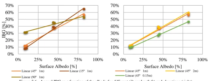
Os resultados mostram que, para uma instalação fotovoltaica típica, o ganho bifacial de irradiância de um único módulo varia entre 37% e 45%, dependendo do ângulo de inclinação. O ângulo de inclinação que maximiza o ganho bifacial de irradiância é geralmente maior do que o ângulo ótimo que maximiza a radiação total intercetada. Módulos mais elevados e solos com maior refletividade aumentam o ganho bifacial de irradiância. Também foi visto que a irradiação intercetada pelo lado traseiro do módulo bifacial é mais homogénea no caso de este estar numa posição de paisagem e não
cada célula solar bifacial.
Relativamente à simulação para um conjunto de módulos bifaciais, as distâncias ideais entre filas e entre painéis numa mesma fila para minimizar a interferência entre eles são superiores ao caso monofacial, e tanto maiores quanto mais refletivo for o solo.
O segundo objetivo da dissertação passa por desenvolver um modelo elétrico com base no qual se pode estimar a produção dos módulos fotovoltaicos bifaciais. Para o efeito, considera-se que uma célula bifacial pode ser representada eletricamente como duas células monofaciais em paralelo, cada uma delas representada pelo circuito equivalente de um díodo. Este modelo foi desenvolvido recorrendo ao software MATLAB® Simulink e foi testado para várias orientações, ângulos de inclinação e posições de montagem.
A partir das simulações efetuadas, verificou-se que, para um módulo bifacial, o ganho bifacial de energia é proporcional ao ganho bifacial de irradiância e ambos aumentam com a fração difusa. Para uma instalação fotovoltaica típica da EDP, o ganho bifacial de energia varia entre 28% a 35%, dependendo do ângulo de inclinação.
Se a orientação do módulo bifacial for diferente da ótima, isto é, se se encontrar orientado a este ou oeste, é possível observar-se alterações da curva típica de produção fotovoltaica, nomeadamente o aparecimento de dois picos, um de manhã e outro ao anoitecer.
Por último, foi avaliado o papel que os módulos bifaciais poderiam ter em soluções de autoconsumo residencial. Os resultados mostram que os módulos solares bifaciais e monofaciais orientados a sul se comportam de maneira semelhante, por unidade de potência instalada, pelo que o maior investimento em sistemas bifaciais não se justifica. Porém, módulos bifaciais na vertical, orientados a este ou oeste, permitem maior consumo de eletricidade gerada localmente, o que pode ser vantajoso dado que a energia excedentária que se vende à rede não é tão lucrativa para o consumidor como a que se deixa de comprar. Os módulos bifaciais na vertical permitem, em média, a redução de cerca 1 kWh/kWp no sistema de baterias, comparativamente com módulos virados a sul e com inclinação ótima, assegurando ainda assim uma taxa de autoconsumo superior a 90%.
Se a comparação entre módulos bifaciais e monofaciais considerar a área de implantação em oposição à potência instalada, a utilização de painéis bifaciais verticais orientados a este ou oeste permite não só aumentar a fração de energia autoconsumida em mais de 10%, relativamente a módulos bifaciais com configuração ótima, mas também diminuir a capacidade do sistema de armazenamento necessária, o que se traduz numa possível redução dos custos associados.
Se o sistema de autoconsumo estiver isolado da rede elétrica, a autossuficiência (i.e. fração das necessidades energéticas do consumidor asseguradas pelo sistema de geração fotovoltaica) garantida por módulos bifaciais orientados a sul é aproximadamente 7% superior à dos módulos monofaciais com a mesma configuração, para a mesma capacidade nominal de armazenamento instalada (kWh).
Finalmente, verificou-se que para soluções de autoconsumo isoladas da rede elétrica, a combinação de módulos fotovoltaicos bifaciais com diversas orientações, nomeadamente virados a sul, a este e/ou oeste, permite obter uma taxa de autossuficiência mais elevada, podendo mesmo aproximar-se dos 100% durante as horas solares aproximar-se a área de módulos e a capacidade da bateria instaladas forem suficientemente elevadas.
Palavras-Chave: Fotovoltaico Bifacial, Modelo de Irradiância, Modelo Elétrico, Autoconsumo,
The concept of using both faces of a photovoltaic module to convert solar radiation into electrical energy emerged at the end of the 20th century and is known as bifacial photovoltaics. Along with the incident radiation on the front side, bifacial solar cells take advantage of the diffuse, reflected and direct radiation that reaches the cell’s active rear side.
This dissertation focuses on evaluating and analysing the differences of using bifacial over traditional monofacial photovoltaic technology, both in terms of collected irradiance and power production. Also, it explores how to integrate this technology with storage to optimize self-consumption solutions.
In this study, the optimum configuration for a bifacial photovoltaic module is investigated numerically, using the software Rhinoceros and Simulink, in order to determine the suitable tilt angle, elevation and mounting position of the module and the ground reflectivity that optimises bifacial gain. Modelling a bifacial photovoltaic system for a case study, Lisbon, Portugal, showed that power production is highly dependent on the incident radiation, stand design and reflectivity of the ground. For a typical photovoltaic plant, the bifacial gain varies from 28%-35% for power production and from 37%-45% for the irradiation received, depending on the tilt angle. Higher stands and more reflective ground surfaces boost the bifacial gains. It is also shown that the electrical generation gain is proportional to the irradiance gain and both increase with the diffuse fraction.
Finally, the analysis of a residential self-consumption solution that seeks to integrate a bifacial photovoltaic installation and batteries showed that south-facing bifacial and monofacial modules behave similarly, with similar yields per unit of power installed. Per unit module area, south facing bifacial solar modules clearly outperform standard monofacial modules, since the self-sufficiency rate (i.e. fraction of the energy demand that is fulfilled by on-site photovoltaic generation) can be approximately 7% higher, for the same nominal capacity of the storage system (kWh).
Results also showed that, the combination of bifacial photovoltaic modules with different orientations, namely south, east and/or west, allows a higher self-sufficiency rate that can almost reach 100% during solar hours, if the module area and storage capacity installed is high enough.
The use of bifacial modules in the vertical, orientated towards the east or the west, increases the fraction of the self-consumed energy in more than 10%, decreasing the excess energy sold to the grid and reducing the required storage capacity, which means the associated costs may be significantly reduced.
Agradecimentos ... iii
Resumo ... iv
Abstract ... vi
List of Figures ... ix
List of Tables ... xii
List of Notations, Abbreviations and Acronyms ... xiv
1. Introduction ... 1
1.1. Solar energy and photovoltaic technology ... 1
1.2. Motivation for bifacial PV ... 1
1.3. Research objectives ... 2
1.4. Dissertation outline ... 3
2. Overview of the bifacial concept ... 4
2.1. History of bifacial technology ... 4
2.2. Bifacial PV technology ... 5
2.3. Working principles ... 7
2.4. Testing modules and standardization ... 7
2.5. Bifacial market and associated costs ... 8
2.6. Modelling a bifacial system ... 10
2.6.1. Irradiance model ... 10
2.6.2. Bifacial cell model ... 12
2.6.2.1. Bifacial electrical model ... 13
2.6.2.2. Thermal model ... 15
2.7. Vertical installations ... 16
3. Irradiance bifacial model ... 18
3.1. Methodology ... 18
3.1.1. Optimization of a bifacial PV installation’s configuration ... 19
3.2. Results and discussion ... 21
3.2.1. Reference module configuration ... 21
3.2.2. Optimization of the configuration for a single module ... 22
3.2.3. Optimization of the configuration for a PV stand ... 26
4. Electrical bifacial model ... 31
4.1. Methodology ... 31
4.1.3. Model dynamics ... 34
4.1.4. Performance indicators ... 35
4.2. Results and discussion ... 36
4.2.1. Performance analysis ... 36
4.2.2. Externalities that affect the bifacial gain ... 42
5. Integration of bifacial PV with storage solutions ... 44
5.1. Methodology ... 44
5.1.1. Self-consumption performance indicators ... 44
5.1.2. Load consumption profile ... 45
5.1.3. Configuration of the PV installation ... 46
5.1.4. Self-consumption installation ... 46
5.1.5. Model dynamics ... 47
5.2. Results and discussion ... 48
5.2.1. PV generation ... 48
5.2.2. Electricity consumption ... 51
5.2.3. Self-consumption system dynamics ... 52
5.2.4. Self-consumption system performance ... 55
5.2.5. Ideal PV technology for a self-consumption solution ... 58
6. Conclusion and further work ... 64
7. Bibliographic references ... 68
8. Annexes ... 72
Annex I – Deduction of the method to electrical characterize bifacial PV modules ... 72
Annex II – Predicted IBG and annual incident irradiation for all the module configurations and ground surfaces in study ... 76
Annex III - PrismSolar® MODEL Bi60-343BSTC ... 86
Annex IV – Predicted energy yield for all the module configurations in study ... 87
Annex V – Daily power density PV curve for the module’s configurations considered for the self-consumption solution ... 88 Annex VI – SSR and SCR for the module configurations and battery capacities in study. 89
CHAPTER 2. Overview of the bifacial concept
Figure 2.1 - Schematic of bifacial solar cell’s architecture proposed by H. Mori. 1 is a n-type thick silicon layer, 2 and 2’ are thin p-type layers, 3 is the negative electrode and 4 is the positive electrode
in contact with the connecting portion of the layers 2 and 2’. [5] ... 4
Figure 2.2 - Cumulative Bifacial PV Installed Capacity. Adapted from [14] ... 5
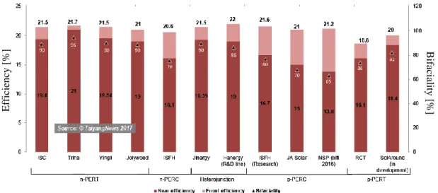
Figure 2.3 - Efficiency and Bifaciality of different bifacial solar cells according to the manufacturer and the architecture. [6] ... 6
Figure 2.4 - Schematic of a bifacial module and the components of the incident radiation on both sides of the module. ... 7
Figure 2.5 - Prevision of the world market share of bifacial solar cells and modules. [15] ... 8
Figure 2.6 - Results of the simulation of LCOE and COO calculation for different technologies. Adapted from [14] ... 9
Figure 2.7 - Geometry for determining the view-factor between the shaded and unshaded region of the ground and the module rear surface. ... 11
Figure 2.8 - Single diode equivalent circuit for a monofacial solar cell. ... 12
Figure 2.9 - Typical equivalent electrical circuit for a bifacial solar cell. ... 13
Figure 2.10 - Absorption behaviour of a monofacial and bifacial cell and a silicon wafer. [42] ... 15
Figure 2.11 – Example of a daily generated power curve for bifacial and monofacial modules with specific orientations, using radiation data from Mito City [47]. ... 17
CHAPTER 3. Irradiance bifacial model Figure 3.1 - Rendering of the Rhinoceros geometry for a single solar cell (a) and a PV module (b) used for incident irradiance estimation. The dimensions are in cm. ... 19
Figure 3.2 - Inter-row and within row spacings visual demonstration. ... 21
Figure 3.3 - Modelled annual cumulative irradiation dependency on the tilt angle for the reference bifacial module (elevation=1m; ground=white gravel; mounting=landscape; orientation=south). Right axis shows irradiance bifacial gain (IBG). ... 22
Figure 3.4 - Inhomogeneity of the radiation on the rear side for two different module’s mounting positions (ground=white painted concrete; tilt=45º; elevation=0.15m). The solar radiant exposure presented is for a year... 23
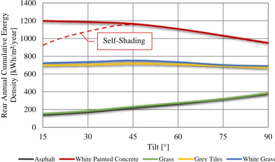
Figure 3.5 - Modelled annual cumulative rear irradiation dependency on the tilt angle for the reference bifacial module (elevation=1m; mounting=landscape; orientation=south). ... 24
Figure 3.6 - Annual IBG as a function of the albedo for different tilt angles (left) and elevations (right). (mounting=landscape; orientation=south) ... 25
Figure 3.7 – Dependency of the annual rear cumulative irradiation (lines) and the IBG (dots) on the elevation and ground surface (tilt=45º; mounting=landscape; orientation=south). ... 26
Figure 3.8 - Effect of the distance between rows in the inhomogeneity of the radiation in the front of the array (left) and in the back (right). The solar radiant exposure presented is for a year. ... 27
Figure 3.9 - Total irradiation loss difference between rows with bifacial PV modules. The same losses for monofacial modules are represented by the dotted line (tilt=45º; elevation=1m; mounting=landscape; orientation=south). ... 28
Figure 3.10 - Effect of the distance between the modules within rows in the inhomogeneity of the rear radiation. The solar radiant exposure presented is for a year. ... 29
Figure 3.11 - IBG difference within a row for different spacing between modules, considering the reference module (tilt=45º; elevation=1m; orientation=south). ... 29
reference model (ground=white gravel; orientation=south). ... 30
CHAPTER 4. Electrical bifacial model
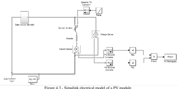
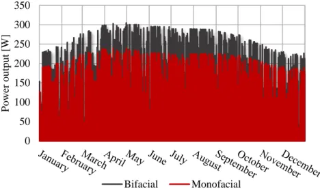
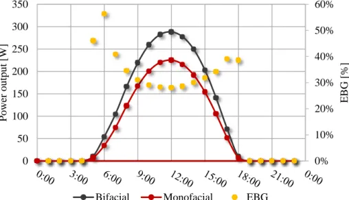
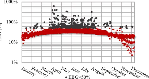
Figure 4.1 - Simulated monofacial (a) and bifacial (b) solar cells in Simulink®. The -C- block represents the input of the hourly irradiance (W/m2) from MATLAB workspace and -BS- converts the input signal to a physical signal. ... 32 Figure 4.2 - Representation of the cell connection path for the monofacial and bifacial PV modules simulated. ... 32 Figure 4.3 - Simulink electrical model of a PV module. ... 34 Figure 4.4 - Flowchart of the algorithm implemented in MATLAB to find the MPP. ... 34 Figure 4.5 - Simulated annual power output for the reference bifacial and monofacial PV modules (tilt=30º; elevation=1m; orientation=south; ground=white gravel). ... 36 Figure 4.6 - Daily variation of the EBG and predicted power production for the reference module on 17/August (tilt=30º; elevation=1m; orientation=south; ground=white gravel). ... 37 Figure 4.7 - Hourly EBG for the reference bifacial module during one year (tilt=30º; elevation=1m; orientation=south; ground=white gravel). A logarithmic scale is applied to the vertical axis for visualization purposes. The black dots represent a divergent behaviour. ... 38 Figure 4.8 - EBG in function of the correspondent hour. The black dots represent a divergent behaviour. (tilt=30º; elevation=1m; orientation=south; ground=white gravel) ... 38 Figure 4.9 - Monthly evaluation of the PR for a single monofacial and bifacial modules with the reference configuration (tilt=30º; elevation=1m; orientation=south; ground=white gravel). ... 39 Figure 4.10 - Annual energy production estimation for monofacial and bifacial modules with the reference configuration (elevation=1m; orientation=south; ground=white gravel). In the right vertical axis is represented the IBG and EBG for the bifacial PV module. ... 39 Figure 4.11 - Daily generated power curve for three bifacial modules with specific orientations and tilt angles on 17/August (elevation=1m; ground=white gravel). ... 41 Figure 4.12 - Representation of the EBG as a function of the IBG for the bifacial reference module (tilt=30º; elevation=1m; orientation=south; ground=white gravel). ... 42 Figure 4.13 - Representation of the EBG as a function of the kd for the bifacial reference module. The black dots represent a divergent behaviour. (tilt=30º; elevation=1m; orientation=south; ground=white gravel). ... 43
CHAPTER 5. Integration of bifacial PV with storage solutions
Figure 5.1 - Annual consumption of the residential sector (profile C) during 2015 [65]. ... 45 Figure 5.2 - Schematic representation of the main components and energy fluxes in a self-consumption installation. ... 47 Figure 5.3 - Flowchart of the algorithm implemented in MATLAB to model the dynamics of a self-consumption with storage system. ... 48 Figure 5.4 - Simulated monthly mean power output normalized by the area for the modules’ types and configurations analysed for a self-consumption solution. The mean values were calculated only for the solar hours. ... 49 Figure 5.5 - PV specific daily production for: (a) 30º South Monofacial; (b) 30º South Bifacial; (c) 90º East Bifacial; and (d) 90º West Bifacial. ... 51 Figure 5.6 - Annual hourly consumption diagram of a typical residential considered for the simulation, throughout 2015. The red dots represent the standard deviation of the hourly energy demand relatively to the monthly average. ... 51 Figure 5.7 - Daily hourly load diagram for the residence of the analysis. ... 52
with 343 W each (17/August). ... 53 Figure 5.9 - Self-consumption dynamic for a system with two 30º monofacial solar modules facing South with 270 W each (17/August). ... 54 Figure 5.10 - Self-consumption dynamic for a system with two vertical bifacial solar modules facing east with 343 W each (17/August). ... 55 Figure 5.11 - SSR in function of the installed PV power for different storage system's capacities, considering 30º south-facing bifacial PV modules. ... 56 Figure 5.12 - SCR in function of the installed PV power for different storage system's capacities. 57 Figure 5.13 - SSR in function of the PV module for different storage system's capacities: (a) 686 Wp PV installed; (b) 2.06 kWp PV installed. ... 58 Figure 5.14 - SCR in function of the PV module for different storage system's capacities: (a) 686 Wp PV installed; (b) 2.06 kWp PV installed. ... 59 Figure 5.15 - SSR in function of the PV module for different storage system's capacities, for an installed PV area of 2.68 m2. ... 60 Figure 5.16 - SCR in function of the PV module for different storage system's capacities, for an installed PV area of 2.68 m2. ... 61 Figure 5.17 – Mean average of the hourly SSR for the different modules’ types and configurations considered, a storage capacity of 1 kWh/kWp and a PV installation area of 2.68 m2. ... 62
CHAPTER 8. Annexes
Figure 8.1 - PV power density daily production for: (a) 30º South Monofacial; (b) 30º South Bifacial; (c) 90º East Bifacial; and (d) 90º West Bifacial. ... 88
CHAPTER 2. Overview of the bifacial concept
Table 2.1 - Empirically determined coefficients used to predict the module's temperature based on the mounting mode and module type [45]. 1 The module is mounted on an open rack allowing air to circulate freely around the module; 2 The module is mounted on a rack with little clearance between the building surface and module’s back allowing little air to flow over the module back; 3 The module is mounted directly to a building surface in a building-integrated PV (BIPV) application preventing air from flowing over the module back. ... 16
CHAPTER 3. Irradiance bifacial model
Table 3.1 - Reflectance, specularity and roughness of the PV materials used in the model. [55] .. 19 Table 3.2 – Overall reflectivity in the RGB visible spectrum of certain ground surfaces according to [55]. ... 20 Table 3.3 - Optimum tilt angle according to the elevation of the PV module and the type of ground surface (mounting=landscape; orientation=south). ... 23
CHAPTER 4. Electrical bifacial model
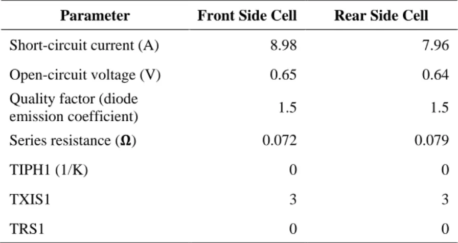
Table 4.1 - Electrical parameters for the front and rear sides of the solar cell introduced in Simulink®. ... 33 Table 4.2 - Annual energy generation and EBG for the reference module in a portrait and landscape mounting position (tilt=30º; elevation=1m; orientation=south; ground=white gravel). ... 40
CHAPTER 5. Integration of bifacial PV with storage solutions
Table 5.1 - Configurations of the PV modules tested to integrate in a PV system with storage. ... 46 Table 5.2 – Specific and absolute energy yield for the modules’ types and configurations analysed for the self-consumption solution. ... 50
CHAPTER 8. Annexes
Table 8.1 - Annual cumulative energy density for the front and rear sides of a landscape solar module above asphalt and correspondent IBG. ... 76 Table 8.2 - Annual cumulative energy density for the front and rear sides of a portrait solar module above asphalt and correspondent IBG. ... 77 Table 8.3 - Annual cumulative energy density for the front and rear sides of a landscape solar module above white painted concrete and correspondent IBG. ... 78 Table 8.4 - Annual cumulative energy density for the front and rear sides of a portrait solar module above white painted concrete and correspondent IBG. ... 79 Table 8.5 - Annual cumulative energy density for the front and rear sides of a landscape solar module above grass and correspondent IBG. ... 80 Table 8.6 - Annual cumulative energy density for the front and rear sides of a portrait solar module above grass and correspondent IBG. ... 81 Table 8.7 - Annual cumulative energy density for the front and rear sides of a landscape solar module above grey tiles and correspondent IBG. ... 82 Table 8.8 - Annual cumulative energy density for the front and rear sides of a portrait solar module above grey tiles and correspondent IBG. ... 83 Table 8.9 - Annual cumulative energy density for the front and rear sides of a landscape solar module above white gravel and correspondent IBG. ... 84
above white gravel and correspondent IBG. ... 85 Table 8.11 - Annual energy converted normalized by the area of the module - Energy Yield (kWh/m2) - or by the peak power - Specific Yield (kWh/kWp) -, for all the module configurations considered in the electrical model. ... 87 Table 8.12 - SSR for a self-consumption system depending on the storage capacity and the configuration and area of the modules installed. ... 89 Table 8.13 - SCR for a self-consumption system depending on the storage capacity and the configuration and area of the modules installed. ... 90
BG Bifacial Gain
BOS Balance of System Costs
BSF Back Surface Field
COO Cost of Ownership
CPC Compound Parabolic Concentrators
DHI Diffuse Horizontal Irradiation
DoD Depth of Discharge
EBG Energy Bifacial Gain
FF Fill Factor
GHI Global Horizontal Irradiation
HIT Heterojunction with Intrinsic Thin layer
IBC Interdigitated Back Contact
IBG Irradiance Bifacial Gain
IR Infrared (radiation)
kd Diffuse fraction
LCOE Levelized Cost of Electricity
MPP Maximum Power Point
NOCT Normalized Operating Cell Temperature
PV Photovoltaic
PERC Passivated Emitter and Rear Cell
PERT Passivated Emitter, Rear Totally diffused
PR Performance Ratio
RES Renewable Energy Sources
RMSE Root Mean Square Error
SCR Self-Consumption Rate
SOC State-Of-Charge
SSR Self-Sufficiency Rate
STC Standard Test Conditions (Cell Temperature = 25ºC, Irradiance = 1000W/m2 and Air Mass 1.5)
1. Introduction
This chapter briefly reviews the use of solar technologies, such as photovoltaic (PV), to provide part of the electricity that humankind requires, and discusses the most relevant challenges and opportunities for the development of bifacial PV. Then, it presents the main research objectives of this dissertation and, finally, the outline of the document.
1.1. Solar energy and photovoltaic technology
The potential shortage of supply to the demand of fossil fuels, as well as the awareness to the environmental impacts caused by their irresponsible and continuous use, has significantly increased the growing interest on more efficient and eco-friendly alternative technologies to convert energy. Photovoltaics is one of the solutions to break the bond once created with fossil fuels and has great potential since the solar radiation is a clean, widely accessible and unlimited energy resource and can address a substantial fraction of the world’s energy demand.
In 2016, PV registered a record annual growth rate of energy capacity, making up about 47% among all Renewable Energy Sources (RES) and totalling a worldwide installed capacity of 303 GW [1]. Despite the positive outlook, solar PV had an estimated share of only 1.5% of the global electricity generation [1]. The Roadmap of Solar Photovoltaic foresees that PV will achieve a 16% share in the global electricity mix by 2050 [2]. In order to reach the objective, it is necessary to reduce the PV capital cost and, simultaneously, increase the generated electricity throughout the system’s lifetime.
Over the last few years, low-cost electricity has increasingly been provided by solar technologies, owing to technological improvements, upgraded financial solutions, manufacturing economies of scale and the expansion into new markets. The continuous research for high tech and materials to make PV cost-effective led to the enrichment of the solar market with a more sophisticated knowledge and efficient use of solar radiation.
The incorporation of bifacial solar cells into glass-glass or glass-transparent backsheet modules is one of the emerging solutions to achieve higher throughput at lower costs. It not only enhances the energy yield of a PV system over its lifetime and its durability (due to a more robust and reliable encapsulation that reduces degradation over time), which allows a reduction of the Levelized Cost of Electricity (LCOE) [3], but also facilitates its incorporation in many applications, e.g. optimizing self-consumption solutions with storage, since these solar modules are able to peak-shift the typical PV production curve.
1.2. Motivation for bifacial PV
Bifaciality opens a new world of possibilities for the traditional PV knowledge, encouraging new investments and the search for a new paradigm.
Despite being relatively expensive, mainly because of the additional manufacturing steps, the requirement for high quality silicon wafers and lacking the opportunities for economies of scale as
standard PV modules do, bifacial technology continues to be investigated to develop more practical and cost-effective solar cells able to take advantage of the incident radiation that reaches their both active surfaces. The simplicity of the concept is attractive, especially because relevant improvements can be achieved merely by adjusting the manufacturing process of advanced cell architectures, which are (in most cases) intrinsically bifacial.
The valuable purpose of using bifacial PV is mainly justified by the energy conversion boost over the system’s lifetime, which strongly depends on the installation configuration and location, and the improved performance and durability. Furthermore, it also enables the Balance Of System (BOS) costs reduction and, hence, the decrease of LCOE. BOS reduction is essentially justified by a decrease of the required area to install the PV power plant and, consequently, the related costs.
In addition, bifacial has an obvious advantage over monofacial PV, since it occupies the same physical area but converts relatively more solar energy into electricity. Consequently, bifaciality can be used to face space limitations in highly populated places (e.g. building integrated PV) or the shortage of suitable sites with a reasonable capacity potential.
Finally, it is important to mention that bifacial can be used in many other applications, even when monofacial would underperform. For example, bifacial modules mounted vertically could be beneficial in terms of increasing dispersed PV generation in space-limited self-consumption systems, since they can easily meet the consumer energy demand peaks in the morning and evening. Besides, they can be installed in multiple applications where single rows of solar modules are appropriate, such as railways and highways, using both surfaces to produce energy.
Nevertheless, as any other new technology trying to enter the market and open roads for widespread use, bifacial faces some challenges related to the inexistence of an international standard for rating the bifacial electrical characteristics, the manufacturing challenges that results in higher modules’ prices and the absence of long-term data to testify the theoretically calculated energy boost. Lastly, there is the necessity to devise a methodology to effortlessly and accurately predict the energy gains in outdoor conditions.
The last point will be one of the main objectives of the present dissertation, which aims to provide the basis for a future performance analysis of bifacial PV technology. Although the results of the simulations performed are purely theoretical, they may be soon used for comparison with real quantitative measurements of the future EDP outdoor facility to test bifacial PV.
1.3. Research objectives
This dissertation explores the potential of bifacial PV installations and its integration with storage solutions. The objectives are three-fold:
i. To evaluate the bifacial PV’s gains,
ii. To suggest the system design that increases the advantage of bifaciality and,
iii. To analyse how to integrate this technology with storage solutions and quantify the advantages comparatively to monofacial PV systems.
To achieve the proposed goals, the work was divided into the following tasks: ▪ Identify the most widely used models to evaluate the performance of bifacial PV; ▪ Analyse the irradiation gain of a bifacial PV module;
▪ Investigate the impacts of relevant factors in the design and geometry of a bifacial power plant, e.g. tilt angle, elevation, ground’s albedo, mounting, intra-row spacing and distance between rows;
▪ Develop a simulation strategy to estimate the energy output of a bifacial system;
▪ Sizing a PV system with storage for a residential consumer and analysing the ideal configuration of the modules and the capacity of the battery.
1.4. Dissertation outline
The outline of this dissertation is as follows.
In chapter 2, a state-of-art overview is given, whereas the principles and challenges of the bifacial PV technology are described as well as the models already proposed for the evaluation of its performance.
Then, the dissertation is divided in three major chapters, according to each one of the subjects analysed and the algorithms implemented. The case study and assumptions made are thoroughly described as well as the simulation input data.
Namely, chapter 3 covers the methodology to predict the incident radiation that reaches both surfaces of bifacial PV modules. The results are also presented, analysed and discussed, focusing on the evaluation of the bifacial gain in terms of irradiance received comparatively to a monofacial PV module and on the determination of the ideal system design and module configuration.
Chapter 4 focuses on the bifacial PV power production and how it is affected by some intrinsic and extrinsic variables to the system itself. After the methodology’s description, the results are analysed based on performance indicators and the influence of some variables on the electrical power production is discussed.
The focus of chapter 5 is to size a residential self-consumption system with storage and analyse its dynamics. The influence of the installed PV power/area and the storage capacity on the capacity to fulfil the consumer energy demand is also determined.
Finally, in chapter 6, the main conclusions of the dissertation are drawn and some recommendations for future work are given.
2. Overview of the bifacial concept
Over the past few years, the PV market and solar manufacturers have shown a renewed and strong interest for bifacial technology. This chapter briefly presents the history and principles of bifacial PV and discusses the most relevant challenges for its development, such as bankability, lack of standardization, associated costs and the modelling and simulation of bifacial PV systems.
2.1. History of bifacial technology
The invention of the bifacial concept is a subject of doubt since it could have been created not to take advantage of the incident radiation on both sides of the solar cell, but as a consequence of the structure and properties of certain types of cells.
The first silicon solar cell was produced in Bell Labs, in 1954, with an n-type Interdigitated Back Contact (IBC) structure [4]. The architecture of this cell allows it to be operated in bifacial mode with two active surfaces. However, credit of the creation of bifacial solar cells goes to the Japanese expert H. Mori [5] and the Russian scientists A.K. Zaitseva and O.P. Fedoseeva [6] who developed the same idea independently. In 1960, H. Mori patented a solar cell with a collecting p-n junction on each side of a n-type silicon wafer, forming a p+np+ structure, and describes the possibility of being double-sided illuminated [7], as can be seen in Figure 2.1. Since then, the efficiency evolved from residual values to 21.3% at the front and 19.8% at the rear side [7].
Many researchers investigated and continue to develop bifacial PV technology. The number and diversity of bifacial solar cell structures is large, with over 166 accumulated patents in 2016a [8]. The path of bifacial design often crosses Heterojunction with Intrinsic Thin layer (HIT), Passivated Emitter and Rear Cell (PERC) and Passivated Emitter, Rear Totally diffused (PERT) solar cells [6].
Since its conception, bifacial technology evolved and many applications were proposed to make use of this innovative idea, including for example its integration in Russian satellites since the 70s [9]. The advantages of using bifacial cells in space instead of monofacial are the enhancement of incident radiation from the Sun and Earth’s albedo and the lower infrared (IR) absorbance that leads to reduced
a The results were obtained for the search terms “bifacial” + “solar”.
Figure 2.1 - Schematic of bifacial solar cell’s architecture proposed by H. Mori. 1 is a n-type thick silicon layer, 2 and 2’ are thin p-type layers, 3 is the negative electrode and 4 is the positive electrode in contact with the connecting portion of the
operating temperature. Nowadays there are still 10 kW bifacial modules installed at the International Space Station, with a proven power generation increase of 10-20% [7].
In terrestrial applications, bifacial started to be used with flat mirrors and, later, with Compound Parabolic Concentrators (CPC), directing sunlight towards the rear side. Only in the early 80s, it was realized that bifacial solar cells were sensitive to natural or artificially enhanced albedo of the environment. Commercial applications have so far been restricted to few niche areas, such as noise barriers on Swiss railways and highways and some research facilities [9]. Still, because of their improved performance and potential, bifacial cells have entered the PV industry and market, although with a relatively low share.
The installation of the world’s first large scale bifacial PV power plant took place in Hokuto, Japan, in 2013, with a total power of 1.25 MW. This plant has reported a bifacial gainb (BG) of 19.5%, producing more than 1.2 MWh/kW/year [10]. Since then, other bifacial power plants were installed in Chile (2.5 MW), in the USA (12.8 MW) [11] and the largest project to date in China (50 MW) [12]. Recently, the Dutch Tempress Systems B.V. inaugurated one of Europe’s largest bifacial PV facilities in Netherlands with 400 kW [13].
Figure 2.2 shows the bifacial systems’ cumulated power since 2012 [14]. As can be seen, the bifacial PV capacity is consistently growing and it is expected that by the end of 2017 the number of bifacial installations will be at least triple relatively to the previous year, since PV manufacturers started to set up bifacial cell capacities [6].
Although bifacial solar cell promoters aim at reaching a leading role in centralized power production, the lack of reliable and long-term field data and the absence of methodologies to assess its annual energy yield gain for a specific installation hinder its global deployment.
2.2. Bifacial PV technology
According to the 2017 edition of International Technology Roadmap for Photovoltaic, the present monofacial silicon solar cell standard technology – Back Surface Field (BSF) – represents a very large percentage of the PV world production (almost 80% in 2016 [15]). Although it reaches high efficiencies
b Bifacial gain quantifies the energy boost due to the use of bifacial PV modules or systems relatively to monofacial
PV. The concept itself will be explained in detail in chapter 4.
0 20 40 60 80 100 120 140 2011 2012 2013 2014 2015 2016 2017 Insta ll ed ca pa ci ty [MW]
(up to 19% at the module level), its performance is limited by recombination at the rear surface and, consequently, it is essential to develop new approaches to produce solar cells with higher efficiencies. A running high efficiency alternative is double-sided contact cell concepts which are intrinsically bifacial [15].
The main difference between conventional monofacial structures and a bifacial cell is that, in the latter, the rear surface must have metal contacts instead of being fully covered by metal (usually an aluminum-based paste). As a result, radiation can be collected both from the front and rear surfaces of the solar cell.
When a PV manufacturer choses to go bifacial, the technical choice is essentially among three structures: HIT, PERT and PERC, each one with different bifaciality levels. Bifaciality is defined as the ratio between the rear side efficiency and the front side efficiency or as the ratio of the power output at STC from the rear side upon the power output at STC from the front side.
Bifaciality = 𝜂𝑟𝑒𝑎𝑟 𝜂𝑓𝑟𝑜𝑛𝑡
= 𝑃𝑆𝑇𝐶,𝑟𝑒𝑎𝑟
𝑃𝑆𝑇𝐶,𝑓𝑟𝑜𝑛𝑡 (2.1)
n-PERT and HIT are the most effective since they have a bifaciality of more than 90%, followed by PERC with 70% [6]. Bifaciality depends strongly on the type of cell as seen in Figure 2.3.
As for the bifacial PV modules, the opaque backsheet must be replaced by an additional glass layer or by an UV-resistant transparent backsheet. Although this type of encapsulation increases the thermal insulation on the back side, bifacial cells still have a lower absorbance relatively to IR radiation, which decreases the temperature of operation comparatively to monofacial PV modules. Besides, it prevents the penetration of water in the module’s interior and reduces degradation over time, increasing the duration of the module [9]. In the case of glass-glass modules, the package is also more rigid, which reduces de mechanical stress on cells [16]. Although these advantages might not be sufficient to switch the typical encapsulation of PV modules (regardless of technology), they come for free in bifacial PV modules, since their rear surface must ensure that the incident radiation can reach the back side of the bifacial PV cells.
In addition, the design of stable mounting systems and junction boxes should be changed to not disturb the light-sensitive areas causing undesirable shading. Furthermore, the junction boxes must handle higher currents [17], [9], [6].
Eff ic ie ncy [%] Bi facial it y [%]
2.3. Working principles
Along with the incident radiation on the front side, bifacial PV take advantage of the diffuse, reflected and direct radiation that reach the module’s active rear side, depending on its orientation, elevation and tilt, site’s characteristics and the position of the sun in the sky, Figure 2.4. Thus, the power output of the rear side is highly dependent upon the local ground’s albedo and its surroundings, the module installation configuration and meteorological conditions. From the shadow region on the ground, only diffuse radiation is captured by the solar module, while in the unshaded area, both direct and diffuse radiation are reflected, affecting the rear side of the bifacial module.
When considering a PV stand, the evaluation of bifacial gains becomes more complex due to the different variables involved, not only the aforementioned ones, but also the packing density (distance between and within rows), the shadows produced by the mounting, the additional shading caused by the neighbouring modules and the obstruction of reflected radiation. These considerations make bifacial PV power plants more sensitive to the installation layout than the traditional ones that integrate monofacial modules.
2.4. Testing modules and standardization
Making an accurate prediction of the annual yield of a PV stand and setting the system design requires a precise and standardized electrical characterization of the solar modules in use. All PV solar cells are characterized by a normalized operating curve obtained under Standard Test Conditions (STC), which correspond to a normal irradiance of 1000 W/m2, an operating temperature of 25 ºC and an Air Mass of 1.5, this allows a fair comparison between the many structures and commercial cells.
Characterizing bifacial solar cells is much more challenging because of the contribution of the rear side’s power production to the measurements. There is no commonly accepted procedure to consider this extra input which affects the estimation of the solar module’s performance.
Some companies are reporting bifacial PV by flashing the front side of the module with 1.1 suns and taping the rear side with a black foil, others are reporting independently the values for both sides of the module obtained at STC by covering one of the surfaces with a non-reflective sheet while illuminating the other one [18]. It was also proposed the simultaneous measurements of both sides with a double-sun simulator [19] and quoting the I-V parameters under different rear illumination conditions [9], which indirectly assesses the interference between both sides.
Figure 2.4 - Schematic of a bifacial module and the components of the incident radiation on both sides of the module. Direct and
Diffuse
Diffuse
Reflected Reflected
Despite all this procedural diversity, the PV community is making an effort to set international testing standards for bifacial modules and lifetime testing conditions [21]. This is a step that can contribute to increase the mass production and deployment of bifacial modules. The “IEC 60904-1-2: Measurement of current-voltage characteristics of bifacial photovoltaic devices” initiated in 2016 is expected to be published in 2018, after the ongoing revision [6].
Besides the obvious consequences of the lack of standardization of the characterization of bifacial PV modules’ performance, it can also be difficult to develop an analytical and electrical model for bifacial PV, since the current and voltage characteristics of the cell are considered as an input, as will be seen in the chapter 4. Also, the indoor characterization is not appropriated to predict the outdoor output of the module due to the inhomogeneous irradiation on the rear side that results in distortions in the I-V curve, often altered by the effect of the module’s by-pass diodes [20].
2.5. Bifacial market and associated costs
The biggest barrier for bifacial PV is the high associated costs related to the cells’ manufacturing and their integration in solar modules, which is one of the main reasons why bifacial has been a technology for niche applications and with a low market share (2% in 2016 [15]).
Since the traditional BSF monofacial cells are being replaced by structures that can be made bifacial, it is expected that bifaciality will become more usual in the PV market and, by 2027, it is expected to reach a promising market share of 30% (cells) and 35% (modules) [15], as Figure 2.5 shows. Until 2021, the market share of bifacial cells will be higher than that of modules since not all manufactured bifacial cells will be integrated into glass-glass or transparent backsheet modules. While there are new companies entering the market, some of the leading PV manufacturers, like SolarWorld® and Yingli®, have expanded their bifacial capacities, estimating that the total capacity for bifacial technology by the end of 2017 will be about 4 GW [6], [21], [22]. Comparatively to the global monofacial PV manufacturing capacity, which is expected to be in the 80 to 85 GW range in 2017 [24], bifacial PV still has a long journey ahead.
The growing market share is also seen as a drop at the production (Cost of Ownership - COO) and electricity costs, which encorages stakeholders to invest in bifacial technology.
The Cost of Ownership, COO, is an indicator of the most cost-effective product from the perspective of a company. Besides taking into account the costs related to the purchase price,
0% 10% 20% 30% 40% 2016 2017 2019 2021 2024 2027 Ma rke t sha re [%]
Bifacial Modules Bifacial Cells
maintenance and operation, this tool also takes the product quality and the failure costs into consideration [24].
The Levelized Cost Of Electricity, LCOE, is the cost per unit of the electricity produced by a system and includes its total life cycle costs, such as the investment, the operation and maintenance costs, etc. It provides an economic assessment to compare various RES with electricity prices. The LCOE’s calculation of a PV system requires a record of the total electricity produced during the useful lifetime and information about the financing, operation and maintenance costs, which are still unaddressed data for bifacial PV. Also, the price of the energy generated by PV that is marketed can vary significantly between countries due to the taxes and feed-in tariffs, reason why these are sometimes omitted from the analysis [14].
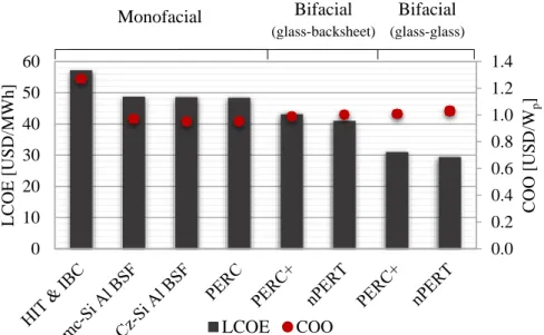
A comparison between monofacial and bifacial PV LCOE and COO was made [14], assuming a power production gain of 20% for PERT and HIT and of 15% for PERC, for a global horizontal irradiation of 1 800 kWh/m2/year and weather conditions similar to the south of Spain (information about the rear irradiation is not given). The module lifetime was assumed to depend mostly on the module technology, corresponding to 25 years for backsheet modules and to 35 years for glass-glass modules, because of their lower yearly degradation rate. For the COO analysis, it was considered a factory located in Asia and an integrated 500 MWp/year cell [14]. The results of the simulation are shown in Figure 2.6.
As seen in Figure 2.6, traditional monofacial technologies are not price-competitive in terms of LCOE and bifacial PV seems to be a promising technology to reduce it (around 14% for glass-transparent backsheet and 25% for glass-glass, the difference is mainly due to the additional 10 years of lifetime), because it increases the energy yield and the lifetime of the system and minimizes the installation area of the solar power plant, thus leading to BOS costs saving, such as land requirement, cabling, etc. However, in terms of cost/Wp, monofacial continues to have the advantage, except for HIT and IBC because of their high-cost manufacturing processes [14]. The COO is more uncertaint and difficult to address particularly because of the lack of standards to quantify the bifacial Wp.
Figure 2.6 - Results of the simulation of LCOE and COO calculation for different technologies. Adapted from [14]
Monofacial 0.0 0.2 0.4 0.6 0.8 1.0 1.2 1.4 0 10 20 30 40 50 60 COO [ US D/W p ] LCOE [ US D/MWh ] LCOE COO Bifacial (glass-backsheet) Bifacial (glass-glass)
2.6. Modelling a bifacial system
The potential of bifacial technology has been demonstrated by simulations and measurements not only for single modules, where energy boosts between 5% [25] up to 54% [26] have been reported, but also for small and larger PV stands, with reported power output increments between 5% and 25% [27], depending on the size of the system. However, these references from literature refer to small systems and the success of bifacial technology depends on demonstrating the same gains on larger scale PV power plants. Bankability, which is the collection of real-world existing bifacial energy-yield data, is one of the challenges that bifacial PV technology has to face in order to facilitate its wider deployment [14].
For a given installation, it is fundamental to accurately predict the energy production and the Bifacial Gain (BG) expected for the various possible stand geometries and different solar cells’ architectures.
The BG is defined as the ratio between the surplus energy produced by bifacial PV and the energy yield of standard monofacial PV, calculated using the following equation.
Bifacial Gain (BG) =𝑒𝑏𝑖−𝑒𝑚𝑜𝑛𝑜
𝑒𝑚𝑜𝑛𝑜 (2.2)
Where 𝑒𝑏𝑖 is the energy yield of bifacial PV and 𝑒𝑚𝑜𝑛𝑜 is the energy yield of standard monofacial PV. The BG can also be calculated in terms of specific yield (Wh/Wp).
The modelling of bifacial PV systems requires the development of a suitable irradiance model as well as a specific electrical model of the bifacial PV modules.
2.6.1. Irradiance model
The irradiance model is required for the prediction of the incident irradiance on the front and rear surfaces of the solar module.
Modelling a bifacial PV system is complex, mostly because the estimation of rear radiation not only depends on correlated variables, such as the location, ground’s albedo and design of the stand, but also due to uneven incident light (caused by shadings of the mounting structure, junction boxes, module frames, irregular reflectors and even the neighbouring modules in the same array). Thus, the model must consider the externalities imposed by the installation’s design, the environment and the shading of the ground and its albedo, and is typically based on two distinct approaches.
The “View-Factor Method” calculates the radiation “emitted” from the underlying surface and received by each cell. The ground beneath the module is divided into two parts: the shaded and unshaded region; in the former only diffuse radiation is reflected, while in the latter both direct and diffuse radiation are reflected. Coding this method is complex, since the view-factors must be calculated for every instant (the position and shape of the shadow change with time due to the motion of the Sun in the sky), it depends on the distance between each cell and the reflective surface and the inhomogeneity caused by the mounting structure cannot be evaluated straightforwardly [11].
Numerically, the view-factor is defined as a geometric quantity that determines the fraction of radiation leaving a surface A1 that directly impinges surface A2. It depends on the relative orientation and distance between the two surfaces and, for finite surfaces, is given by
𝑉𝑖𝑒𝑤 𝐹𝑎𝑐𝑡𝑜𝑟𝐴1→𝐴2= 1 𝐴1∫ ∫ 𝑐𝑜𝑠𝜃1× 𝑐𝑜𝑠𝜃2 𝜋𝑟2 𝑑𝐴2𝑑𝐴1 𝐴2 𝐴1 (2.3) Where 𝑟 is the distance between the differential areas 𝑑𝐴1 and 𝑑𝐴2 and 𝜃1 and 𝜃2 are the angles between the normal vectors of the surfaces and the line that connects 𝑑𝐴1 and 𝑑𝐴2, respectively.
EDF R&D applied this model to a single module [26]. After calculating the view-factors between the illuminated ground and the module and between the shadowed ground and the module, the total irradiance on the rear surface is given by the flux of direct, diffuse and reflected irradiance (both from the shaded and unshaded regions). The mean error varied between 1% and 3%, depending on the configurations considered and the irradiance level, but the absolute error reached almost 15%, when compared with measured data. Applying the same model to a string of modules resulted in a Root Mean Square Error (RMSE) of 18.9 W/m2, i.e. 14% relatively to the mean of the measured values [28].
At the Sandia PV facility constructed in 2016 for testing bifacial PV modules, the back-surface irradiance was also modelled by the “View-Factor Method” for cells installed near the middle of each row, at the top and bottom of the module. Considering only the rear irradiance, the RMSE varied between 4.8 W/m2 and 16.5 W/m2, being the deviation of the measured value from the modelled value higher for the top cells [29].
The same approach was used by a partnership between ISC Konstanz and some universities in Germany [30], [31] and J. Appelbaum from the School of Electrical Engineering in Israel [32] to determine the input to the electrical model.
The second approach is called “Ray-tracing Method” and uses a 3D modelling software with a daylighting and energy modelling plug-in. The simulation tool provides a precise and realistic rendering of the PV system and radiation map distribution and can calculate the reflections between surfaces based in their reflectivity. Commonly, the software uses an illumination model based on Perez model for direct and diffuse irradiance that assumes the sky is isotropic for all weather conditions and all module’s orientations [33]. It was tested, for example, by a group of researchers from NREL, Iowa University and Sandia National Laboratories [34] and by Fraunhofer Institute for Solar Energy Systems [27]. EDF calculated the RMSE of the method as 15.7 W/m2 which was found to be close to the pyranometers’ uncertainties [35].
Figure 2.7 - Geometry for determining the view-factor between the shaded and unshaded region of the ground and the module rear surface.
For simple cases, there is a good agreement between the two methods [35], but as the complexity increases, their pros and cons become more noticeable. For the “View-Factor Method”, as the size of the system becomes larger and there are more externalities to take into account (e.g. structures that cause shading, as the module frame and the mounting assembly), the processing time and complexity increases. As for the “Ray-tracing Method”, it offers a great flexibility and accuracy in the prediction of the incident irradiance, it also allows the representation of several configurations, surface properties and considers the impact of inhomogeneous radiation, reflection and shading. Nevertheless, the computational representation of the system cannot be generalized to every PV stand or location, i.e. it is not universal, since it must reliably represent the real system, assuming it is already implemented, which may not be the case.
2.6.2. Bifacial cell model
The rear and front radiation estimated by the irradiance model will be directly introduced as an input in the electrical model to obtain the simulated bifacial power production. The system’s characteristics that englobe the details of the module performance and the system installation are also included in the electrical model.
Almost all electrical devices can be represented by a minimalist electronic circuit. Monofacial solar cells are usually modulated by a single diode equivalent circuit, shown in Figure 2.8, because the characteristic I-V curve of an illuminated solar cell behaves as an ideal diode affected by a series and shunt resistances [36]. The presence of a shunt resistance is typically justified by manufacturing defects which provide alternative paths for the generated photocurrent, while the series resistance is caused by many effects such as the resistance experienced by charge carriers in the p-n junction and the contact resistance in the interface between the semi-conductor material and the metal contact and the resistance of the metal contacts.
The I-V characteristic equation of the single diode equivalent circuit is formulated from Kirchhoff’s current law and given by
𝐼 [𝐴] = 𝐼𝑝ℎ− 𝐼0[exp (
(𝑉 + 𝐼𝑅𝑠)
𝑛𝑉𝑇 ) − 1] −
𝑉 + 𝐼𝑅𝑠
𝑅𝑠ℎ (2.4)
where 𝐼𝑝ℎ is the photocurrent generated, 𝑉𝑇 is the thermal voltage dependent on temperature, 𝐼0 is the diode reverse saturation current and 𝑛 its ideality factor.
Sometimes, for better accuracy, particularly for low irradiation conditions, a two-diode equivalent circuit is used rather than a single diode. While the first diode is used to represent the Shockley-Read-Hall recombination in the space charge region, the second diode is used to model the recombination
processes, such as Shockley-Read-Hall and Auger, elsewhere, in the base and emitter or in the front and rear surfaces [37].
2.6.2.1. Bifacial electrical model
Different electrical models of bifacial solar cells have been proposed, developed and tested to predict its power production output. Most of the models developed consider that a bifacial solar cell can be represented as two monofacial cells in parallel, represented by the single diode or two-diodes equivalent circuit. The electrical diagram of the model is presented in Figure 2.9.
The number of possible combinations for the incident radiation at the front and rear sides of a bifacial module is virtually infinite, so it is neither practical nor feasible to determine the electrical parameters of the PV module for all those conditions.
J. Singh et al. have synthesized a method to electrically characterize bifacial PV modules for all illumination conditions [38]. The basis is the one-diode model of a monofacial cell and the electrical parameters given as an input to the model are extracted from the I-V curves obtained independently for the front and rear sides of the cell at STC. Therefore, the interference between both sides is not considered, which can lead to slight deviations between the experimental data and the simulation results. These extracted parameters include the short circuit currents, 𝐼𝑠𝑐,𝑓𝑟𝑜𝑛𝑡 and 𝐼𝑠𝑐,𝑟𝑒𝑎𝑟, and open circuit voltages, 𝑉𝑜𝑐,𝑓𝑟𝑜𝑛𝑡 and 𝑉𝑜𝑐,𝑟𝑒𝑎𝑟, for front and rear sides of the bifacial solar cell, respectively.
The method assumes a linear response of the short circuit current for different radiation levels and considers bifacial as a monofacial module operating at a current which is the sum of the currents generated independently by the front and rear sides, because once the charge carriers have been generated, it makes no difference to the cell from which side the incident radiation entered. In order to define some parameters, the model also defines the irradiance ratio as the ratio of rear and front irradiances, as following [38]:
𝐼𝑟𝑟𝑎𝑑𝑖𝑎𝑛𝑐𝑒 𝑅𝑎𝑡𝑖𝑜 (𝜒) = 𝐺𝑟𝑒𝑎𝑟
𝐺𝑓𝑟𝑜𝑛𝑡 (2.5)
where 𝐺𝑟𝑒𝑎𝑟 and 𝐺𝑓𝑟𝑜𝑛𝑡 are the incident irradiances on the rear and front sides, respectively.
The power of bifacial modules can be defined as follows:
𝑃𝑏𝑖𝑓𝑎𝑐𝑖𝑎𝑙 = 𝐼𝑠𝑐,𝑏𝑖 𝑉𝑜𝑐,𝑏𝑖 𝐹𝐹𝑏𝑖 (2.6)
with 𝐼𝑠𝑐,𝑏𝑖, the short circuit current for bifacial modules, defined using the notion of short circuit current gain (ℛ𝐼𝑠𝑐) relative to monofacial PV:
𝐼𝑠𝑐,𝑏𝑖 = ℛ𝐼𝑠𝑐 𝐼𝑠𝑐,𝑓𝑟𝑜𝑛𝑡 = (1 + 𝜒 𝐼𝑠𝑐,𝑟𝑒𝑎𝑟
𝐼𝑠𝑐,𝑓𝑟𝑜𝑛𝑡) 𝐼𝑠𝑐,𝑓𝑟𝑜𝑛𝑡 (2.7)
The bifacial open circuit voltage, 𝑉𝑜𝑐,𝑏𝑖, is
𝑉𝑜𝑐,𝑏𝑖 = 𝑉𝑜𝑐,𝑓𝑟𝑜𝑛𝑡+(𝑉𝑜𝑐,𝑟𝑒𝑎𝑟− 𝑉𝑜𝑐,𝑓𝑟𝑜𝑛𝑡)ln (ℛ𝐼𝑠𝑐)
ln (𝐼𝑠𝑐,𝑟𝑒𝑎𝑟 − 𝐼𝑠𝑐,𝑓𝑟𝑜𝑛𝑡) (2.8)
And the bifacial fill factor, 𝐹𝐹𝑏𝑖 is
𝐹𝐹 𝑏𝑖 = 𝑝𝐹𝐹 − ℛ𝐼𝑠𝑐𝑉𝑜𝑐,𝑓𝑟𝑜𝑛𝑡
𝑉𝑜𝑐,𝑏𝑖 (𝑝𝐹𝐹 − 𝐹𝐹𝑓𝑟𝑜𝑛𝑡) (2.9)
In Equation 2.9, 𝑝𝐹𝐹 is the pseudo Fill Factor (FF) of the module considering no series resistance loss which can be calculated using Equation 2.10.
𝑝𝐹𝐹 =(𝐼𝑠𝑐,𝑟𝑒𝑎𝑟/𝐼𝑠𝑐,𝑓𝑟𝑜𝑛𝑡)𝐹𝐹𝑓𝑟𝑜𝑛𝑡− (𝑉𝑜𝑐,𝑟𝑒𝑎𝑟/𝑉𝑜𝑐,𝑓𝑟𝑜𝑛𝑡)𝐹𝐹𝑟𝑒𝑎𝑟
(𝐼𝑠𝑐,𝑟𝑒𝑎𝑟/𝐼𝑠𝑐,𝑓𝑟𝑜𝑛𝑡) − (𝑉𝑜𝑐,𝑟𝑒𝑎𝑟/𝑉𝑜𝑐,𝑓𝑟𝑜𝑛𝑡) (2.10)
This method has been shown to estimate the power output within 1% of measured results, for different sets of irradiance conditions [43]. Its demonstration can be found in Annex I – Deduction of the method to electrical characterize bifacial PV modules.
A collaborative investigation developed by ISC Konstanz and University of Stuttgart used a simplified version of the model suggested by Singh et al., considering FF as a fixed value measured at STC, which leads to an overestimation of the output power for high irradiance levels and an underestimation for low irradiance levels. Although the good agreement between the measured and simulated BG proves the reliability of the model, the authors defend that the simulation tool requires some improvements, which include quantifying the daily and seasonal variation of ground’s albedo (counting the influence of the diffuse fraction and the solar zenith angle), develop a more accurate electrical model and considering shadowing effects [30].
The aforementioned analytical model gives accurate modulation for homogeneous irradiance conditions, but it does not take into account the possible electric current mismatch in different cells in the module due to the inhomogeneous patterns of intercepted radiation. Besides, the temperature of a cell can also influence the power production and this effect is not included in the model. These conditions are difficult to address analytically with the previous model without being onerous and time-consuming. For this reason, numerical PV simulation software has been used to predict the enhanced output of bifacial modules dates since 1993 [39].
P. Dupeyrat et al. developed a bifacial solar cell electrical model on Modelica/Dymola® based on the two-diode approach. This model was used to study the influence of the tilt angle and several albedos in three different locations. The results indicate that the BG in terms of energy yield is highly dependent on the aforesaid variables, and the higher values are obtained for places where the global irradiance is predominantly diffuse and installations with more reflective underlying surfaces. [26]
![Table 3.2 – Overall reflectivity in the RGB visible spectrum of certain ground surfaces according to [55]](https://thumb-eu.123doks.com/thumbv2/123dok_br/15450804.1027442/36.892.265.631.329.498/table-overall-reflectivity-visible-spectrum-certain-surfaces-according.webp)