MSc in Finance
How to Profit from Mutual Fund Performance Persistence?
David Rafael Viegas Teodósio Wessling
Advisor:
José Afonso de Carvalho Tavares Faias
Dissertation submitted in partial fulfillment of requirements for the degree of MSc in Finance, at the Universidade Católica Portuguesa,
i
Abstract
How to Profit from Mutual Fund Performance Persistence?
David Rafael Viegas Teodósio Wessling
This thesis demonstrates that mutual fund performance persistence can be profitably exploited with a simple investment strategy. Funds are invested based on the top decile of an ex-ante raw returns rank. Strategy was tested under diverse circumstances and in different fund categories. It is demonstrated that strategies with shorter estimation and rebalancing periods – up to 1 year and 6 months respectively – consistently outperform the respective benchmarks, reaching annualized returns and Sharpe ratios of up to 24.3% and 0.89 respectively. Results are robust across all fund categories with over 42% of the risk-adjusted results being statistically significant. Robustness was also confirmed in expansion and recession periods, with weaker results in the later. It was shown that with transaction costs strategy returns are partially eroded, being the shorter rebalancing strategies – 1 month - the most affected. However it is proved that under realistic circumstances the best performing strategies still outperform by far the respective benchmarks.
ii Acknowledgments
Foremost, I would like to thank Professor José Faias my academic advisor. His dedication, knowledge and unconditional support throughout all phases of this master thesis contributed significantly for the quality achieved. Further I convey my thanks to Professor Carlos Rondão for his readiness to help in programming issues.
Additionally, I would like to express my sincere thanks to Millennium BCP’s Wealth Management team. Especially Mark Dwyer, José Nuno Gago, José Rodrigues, Isabel Simões Reis, Rita Appleton and Nuno Botelho for allowing me to access the funds’ database and for the permanent kindness and technical support. Further thanks to David José Ribeiro for your help.
Above all, I would like to show my sincere gratitude to my family and friends, thanking the patience and dedication they had for me. Especially to my supporting girlfriend Rita Martins, my parents Fritz and Fernanda Wessling and my brother and sisters Pedro, Ana and Susana Wessling to whom I dedicate this thesis. Particular thanks also to my friends that inspired me throughout my academic and personal path, namely Alberto Ippolito, Estela Lucas, Ricardo Pereira and many others.
Finally I would like to thank Católica-Lisbon for all the knowledge conveyed and inspiration for this thesis that is not more than your own merit as well.
iii
Table of Contents
_Toc313831315
I. Introduction ... 1
II. Data & Methodology ... 3
2.1 Mutual Funds Data ... 3
2.2 Performance Persistence ... 10
2.3 Strategy Methodology... 11
III. Results ... 13
3.1 Strategy Results ... 13
3.2 Funds Invested Analysis ... 17
IV. Robustness ... 20
4.1 Strategy in expansion vs. recession periods ... 21
4.2 Strategy vs. Buy and Hold ... 25
4.3 Investment Strategy for Private Investors ... 27
V. Conclusions... 31
iv
List of Tables
Table I - Equity Mutual Fund Database Summary Statistics ... 5
Table II– Performance Measures Summary Statistics ... 7
Table III - Return Persistence – Lagged Autocorrelation ... 10
Table IV - Strategy Results Summary ... 14
Table V - Portfolio Turnover ... 18
Table VI - Strategy Performance Test: Expansion Periods ... 22
Table VII - Strategy Performance Test: Recession Periods ... 23
Table VIII - Index Performance: Expansion and Recession Periods ... 24
Table IX - Impact of Transaction Costs in the Strategy – Performance Loss ... 29
List of Figures
Figure 1: Strategy Diagrams ... 11Figure 2: Sector Funds Strategies - Performance between Jan. 2008 and Dec. 2010... 20
Figure 3: Strategy vs. Buy and Hold Index ... 25
1
I.
Introduction
Fund of funds (FOF) managers and other investors strive to identify and select skilful fund managers that deliver positive alphas by outperforming their passive benchmarks. However the existence of this skill (also known as performance persistent) is a subject of much debate in the industry, being consensus far from reached. Authors like Grinblatt and Titman (1989, 1992), Hendricks et al. (1993), Gruber (1996), Zheng (1999), Bollen and Busse (2004), Fortin and Michelson (2010) found using different approaches that persistency is mainly short termed (estimation periods of at most 1 year). In turn Carhart (1997) argues that persistency in expense ratios drives much of the long-term persistence in mutual fund performance. Further, Jensen (1969) could not find relation between past and future performance whereas Fama and French (2010) acknowledged that if there are skillful fund managers that attain constant positive excess returns, they are hidden in the aggregate of those who can’t, being this a “zero sum” game – zero aggregate α before costs. Moreover they argue that mutual fund performance persistence has a lack of evidence support once the allocation to winner and loser funds is largely based on short-term noise.
The contribution of this thesis goes beyond a simple replication of past studies, differing from previous studies by employing funds from more than one specific region/country, whereas many different studies analyze separately mutual funds from US, UK, Europe, etc. Additionally a thorough cross-sectional analysis is provided by grouping funds into smaller clusters according to their intrinsic characteristics such as type of assets invested, geographic and industry focus. Moreover the key feature of this thesis is the fact that unlike many other studies is endowed with extensive practical relevance to the industry by providing investors with a valid and easily implementable robust investment strategy tested across different types of funds and markets.
This thesis pretends to show that mutual fund performance persistence indeed exists and that it can be exploited with an investment strategy. A very thrilling aspect of this investment strategy is being simple and very straightforward to implement. In short this investment strategy consists on investing in top decile funds of a predetermined estimation period. These funds are invested in an equally weighted basis, meaning that at each period
2
the top decile is composed by N funds being each one’s weight of . Hence any utility maximization or other complex estimation method is avoided, allowing this strategy to be easily understandable and replicable by any investor.
With respect the performance evaluation of both the initial fund categories and the investment strategy, this thesis presents another improvement comparing with previous studies. The factors used in the Carhart’s 4-Factor Model are Global Factors, being this coherent with the worldwide fund-focus approach adopted.
This thesis demonstrates that the consistent best performing strategies are those with shorter estimation and rebalancing periods – up to 1 year and 6 months respectively. These results are consistent with previous authors’ findings such as Hendricks et al. (1993), Gruber (1996), Zheng (1999), Bollen and Busse (2004) and Fortin and Michelson (2010) which support the existence of a short term lived mutual fund performance persistence. These strategies obtain annualized returns and Sharpe ratios of up to 24.3% and 0.89 respectively, outperforming notoriously the respective benchmarks. Results are robust across all fund categories; over 42% of the risk-adjusted results are statistically significant. Strategy’s robustness was also confirmed in expansion and recession periods, with weaker results for the later – outperformance in 79% of the results during expansions and 50% in recessions.
The application of this strategy to private investors faces new challenges such as transaction costs that institutional investors are exempt of. It is showed that strategies hold in presence of transaction costs, even-though their performance is partially eroded. Shorter rebalancing strategies –namely 1 month – are the most affected. However it is proved that under realistic circumstances that take into consideration the fund turnover at each rebalancing event, the best performing strategies still outperform by far the respective benchmarks.
Section II presents the data and methodology of this thesis, detailing on the data sources and sampling procedure. Each fund group will be characterized with respect to quantitative, statistical and performance measures. Further, section III shows the results of the strategy developed for the different fund categories, providing additional detail on fund turnover of the invested portfolio. Moreover, section IV performs robustness tests on
3
the results achieved by endowing a closer insight on the results’ features and resilience in different timeframes. Finally section V provides this thesis’ conclusions and some research future “avenues” that illustrate aspects of this thesis that could be further developed.
II.
Data & Methodology
2.1 Mutual Funds Data
For the purpose of this study monthly mutual fund raw returns – net of fees – from July 1991 to December 2010 were extracted from Lipper Database. By ignoring data prior to 1991 it was possible to circumvent the data selection bias suggested by Carhart (1997) that Lipper Database understates the total number of mutual funds by about 100 each year. For the purpose of this novel strategy solely equity actively managed mutual funds were considered, excluding thus ETF’s. Funds with less than 25 monthly returns up to December 2010 were excluded, allowing for representativeness of fund’s performance record in the statistics performed. This exclusion criterion is coherent with several other papers like Avramov and Wermers (2006), Gruber (1996) and Zheng (1999). From a universe of 7,126 equity funds the sample was reduced to 5,335 illegible funds from which 1,609 (30%) are currently dead. With the 234 months it was possible to have more than 508,000 month-fund return observations. Survivorship bias was purged using standard techniques, i.e. including in the sample the returns of each fund up to the period of disappearance.1
From a 5,335 mutual overall fund universe, clusters were constructed following 3 distinct criteria; size of assets invested by the fund – small & mid cap funds and large cap funds; geographic focus of the fund – global, north American, European, Japan and emerging market funds; and finally sector funds. All in all 9 categories were studied throughout this thesis, the 8 mentioned before plus one that includes all 5,335 equity mutual funds. The fund allocation to each cluster was based on Lipper´s fund classifications “Lipper Global”. The choice upon this geographic and asset-type variety of mutual funds comes from the belief that as integrated global markets are, investors are able to choose where to invest.
4
Thus it would be very restrictive applying the investment strategy solely to the one country/geographic location (ex: US mutual funds) like some previous studies do.
For each one of the 9 categories defined a representative return time series was constructed in an equally weighted (EW) basis, meaning that at each month the category’s return is the equally weighted average return of the existent funds at that month. As an example the return of the European Funds cluster for July 1991 is the arithmetic average (EW) of the returns from the 68 funds that were operating at that time. Data limitations impeded value-weighted (VW) strategies to be tested since it was not possible to access to fund’s assets under management.
Table I describes the summary statistics of the 9 different fund categories. The characteristics of each can be assessed such as size, average number of living funds each month, mean return, volatility of the returns. Performance measures were also calculated: the Sharpe ratio given by formula (1) presents risk return relation, showing the excess return received by a mean variance investor per unit of risk:
(1)
The usual Sharpe ratio implies that returns are i.i.d. however, in the presence of statistical significant serial correlation of the returns a correction has to be made. Therefore Sharpe ratio will be annualized following Lo´s (2002) recommendation by multiplying by instead of multiplying it by , where:
, (2)
and is the statistical significant k-lagged serial correlation and q is the number of correspondent periods that compose a year (e.g. monthly observations q = 12). In the absence of statistical significant correlation note that is zero, being . As an example one could think of annualizing a monthly Sharpe ratio, thus by assuming returns to be i.i.d. the procedure would be multiplying it by . However in the presence of serial correlation of the returns the Sharpe ratio is annualized multiplying it by .
5
Other performance measure used was the certainty equivalent (CE) of the power utility function:
, (3)
where is the coefficient of risk aversion ( , and is the
return of the strategy at time t.2 The certainty equivalent of the power utility function denotes the riskless return perceived by an investor moments of the distribution are taken into consideration. The advantage of this measure over the mean variance certainty equivalent is the fact that takes into consideration all moments of the distribution whereas the mean variance measure just incorporates the first two moments. Moreover the Sharpe ratio is a mean variance measure, thus by employing the power utility certainty equivalent the risk adjusted performance measures became more embracing.
Table I
Equity Mutual Fund Database Summary Statistics
This table presents summary statistics for mutual fund raw returns between July 1991 and December 2010. The # Funds comprehend the Mutual Funds that completed the minimum required 25 monthly returns; Mean # funds is the average number of living funds at each one of the 234 monthly observations; The is the annualized mean return of each group of funds’ EW monthly observations; The is the annualized standard deviation of the monthly EW return observations; SR and CE are respectively the annualized Sharpe ratio and certainty equivalent, Skew and Kurt measure respectively the skewness and kurtosis of the monthly observations; Percentile Mean Returns gives the EW fund mean return for a certain decile. The symbols ***, ** and * denote the statistical significance of the coefficient at 1%, 5% and 10% significance level respectively.
2
See Ferreira and Santa-Clara (2011). For the average stock market excess return and risk a coefficient ( ) of 2 is in accordance to an investor that allocates his entire wealth to the stock market.
Group # Funds Mean # Funds (%) (%) SR CE (%) Skew Kurt Percentile Mean Returns (%) 1 Median 99 All Equity Funds 5,335 2,175 7.9*** 15.0 0.25 5.7 -0.77 4.76 -34.3 3.1 36.6 By asset invested:
Small & Mid Cap Funds 356 164 9.1*** 16.3 0.28 6.6 -0.61 5.02 -33.1 6.6 35.5
Large Cap Funds 4,979 2,011 7.8*** 15.0 0.25 5.6 -0.76 4.71 -34.2 3.6 36.4 By geographic focus:
Global Funds 1,189 436 6.2*** 13.6 0.18 4.4 -0.87 4.75 -41.4 1.9 25.9
North America Funds 563 250 8.3*** 14.6 0.29 6.3 -0.77 4.22 -24.1 2.6 18.9
Europe Funds 1,353 588 8.4*** 15.5 0.27 6.1 -0.73 4.68 -31.9 3.3 28.1
Japan Funds 311 142 0.4 18.3 -0.12 -2.9 0.14 3.32 -39.7 -2.1 12.3
Emerging Mkts. Funds 1,242 145 12.2*** 21.1 0.47** 7.9 -0.52 4.62 -26.6 11.5 42.9 Sector Funds 650 249 8.5*** 16.0 0.27 6.0 -0.66 4.20 -43.6 3.6 45.7
6
There other and more complex ways of computing certainty equivalents however since the one used suits perfectly its purpose makes no sense to use more complicated ones.
Table I further characterizes the return distribution of each group of funds with the skewness, kurtosis and the ranked fund returns in percentiles. Looking at table I it is possible to draw some conclusions on the different fund categories. The first one is the return spread across the different clusters where emerging markets and small & mid cap funds’ categories show great aggregated returns – 21.1% and 16.3% respectively – whereas Japan and global funds’ samples present the poorer returns – 0.4% and 6.2% respectively. This evidence is also reflected in other measures such as the annualized Sharpe ratio and certainty equivalent. If the quality of the aggregated returns were expected for the two samples mentioned above due to the intrinsic features of the stocks invested, the same cannot be said about the global funds sample poorer performance. The Japan funds’ sample is a particular case since the timeframe used captures most of the Japanese Crisis that started after the summer of 1990 and lasted for most of that decade. As a background comparison one should notice that the Nikkei 225 Index was in July 1991 roughly 3 times higher that it was at the time this thesis was written. Other aspects that can be drawn from table I is the fact that large cap category equals all funds’ excluding small & mid cap fund cluster – looking at # funds 4,979 equals 5,335 minus 356. The reasoning for assuming that all non-small or mid cap funds are large cap ones is driven by two main factors; first the difficulty to construct a large cap sample through Lipper classifications since it would exclude many large cap funds. Secondly, this assumption is quite accurate since the large cap sample includes funds that invest solely in large cap stocks and those that invest in all types, being the weight of large cap equities on this second group of funds very significant. Therefore the bias caused by this assumption is minimal comparing with the one that would be caused if the alternative option (using Lipper Global classifications) was employed.
To evaluate the performance of each sample a set of preliminary statistics was completed and each fund group’s EW returns was regressed by OLS against the Carhart´s (1997) 4-Factor model, as can be seen in (4).3
7
; (4)
This model is the Carhart’s 4-Factor model, being constructed from the Fama and French (1993) 3-Factor model by adding a fourth factor – Momentum factor. This model evaluates the performance by comparing it with 4 risk factors where is the return of sample S at
time t and the one-month T-bill rate. The RM-Rf, SMB, HML and WML factors can be seen as passive benchmarks for 4 distinct investment strategies, market return, small versus large capitalization stocks, growth versus value stocks and momentum stocks. Therefore manager that attains his return solely by following these strategies is not considered to have stock selection skills, solely benchmark mimicking ones.
All in all SMB, HML and WML represent value-weighted zero investment portfolios where SMB is the excess return of small cap stocks over large cap one, being long in the former and short in the later. HML represents the excess return of high book-to-market stocks (long position) over low ones (short position). WML corresponds to the excess return of the stocks with high eleven-month returns (lagged 1-month) over the lower ones, meaning that winner stocks are those which positive returns tend to be followed by positive returns and loser stocks those with negative stock return succeeding negative ones. The slopes each factor’s coefficient ( , , h and ) replicate the fund’s exposure to each passive
benchmark. The regression intercept ( ) is the average return left unexplained by the
factors, i.e. the average return of the fund in excess to a comparable passive portfolio, traducing if positive managers’ “stock picking” skill.
Table II shows the estimates for the regression (4) in each one of the 9 mutual fund groups. Each factor coefficient and R2 states respectively the fund category’s exposure to the different benchmarks and regression fit. The annualized alpha expresses each cluster’s returns left unexplained by regression (4), thus a positive statistical significant alpha suggests the existence of skilful funds. Furthermore it is presented the percentage of total funds in each sample which contain statistical significant positive alpha, i.e. stock selection skill (% α > 0**), see also Barras, et al. (2010).
8 Table II
Performance Measure Summary Statistics
This table presents summary performance statistics for different fund categories respecting the period from July 1991 to December 2010. The Ann. α corresponds to the annualized Carhart's 4-Factor alpha (in percentage). RM-RF, SMB, HML, WML factors are the passive benchmarks for 4 distinct investment strategies, market return, small versus large capitalization stocks, growth versus value stocks and momentum stocks. The R² gives the fit of the 4-Factor regression (in percentage) and α > 0** is the percentage of the sample's funds that have a positive alpha significantly different from zero at 5% significance. The symbols ***, ** and * denote the statistical significance of the coefficient at 1%, 5% and 10% significance level respectively.
Group Carhart's (1997) 4-Factor Model
Ann.α RM-Rf SMB HML WML R² % α > 0** All Equity Funds 1.9 0.82*** 0.10* -0.07 -0.09*** 77.3 7.2
By asset invested:
Small & Mid Cap Funds 2.4 0.88*** 0.50*** -0.03 -0.07* 78.9 7.6
Large Cap Funds 1.9 0.82*** 0.07 -0.07 -0.10*** 76.6 7.2
By geographic focus:
Global Funds 1.0 0.74*** 0.04 -0.11* -0.09*** 77.5 1.6
North America Funds 3.4* 0.76*** -0.13** -0.17** -0.10*** 75.3 4.1
Europe Funds 2.6 0.77*** 0.03 -0.05 -0.10** 63.4 2.3
Japan Funds -8.6** 0.82*** 0.43*** 0.19 0.03 45.7 0.0
Emerging Markets Funds 7.6** 1.04*** 0.28*** 0.08 -0.11* 61.2 18.7 Sector Funds 4.3** 0.83*** 0.17*** -0.24*** -0.13*** 77.7 10.6
Three main conclusions can be drawn form table II; (1) annualized alpha is only statistically different from zero in the North America, emerging markets, sector and Japan funds’ categories, suggesting a higher concentration of skilful funds in the first three clusters and unskilled ones in the later (being Japan’s special circumstances discussed briefly later); (2) the regressions have quite large explanatory power with R2´s between 60 and roughly 80 percent – except for Japan – being the majority of the factors statistical significant; (3) in each sample of funds it is only possible to find a small segment of skillful funds (α>0**), exception are the emerging markets and sector funds’ categories.
These results can be partially compared with previous studies since the focus on mutual funds in different geographic locations is difficult to find in the literature. Most studies focus on funds that invest in U.S. common stock, thus it is possible to compare those results with the North America funds group. Fama and French (2010) reached values that present significant differences from those attained in the North America funds cluster. The annualized alpha net of fees is -0.92%, the coefficients of the four factors presented also
9
differences in scale and some in signal. An explanation for these differences is the fact that the factors used in this thesis are global instead of US, being the R2 attained significantly lower than the Fama and French’s (2010) one - 0.98. These differences almost vanish when the returns of North America cluster are regressed against US-Factors.4
All coefficients become very close with annualized alpa of -1.25% and R2 of roughly 0.95. Similar results were achieved by Kacperczyk et al. (2008) that with a comparable timeframe achieved an annualized 4-Factor alpha of -0.82%. The remaining differences may reside first on the fact that unlike the other studies mentioned, the North America fund cluster presented in this thesis includes Canada´s funds and second on the existence of small differences in the time-frames used between studies. Nevertheless it can be seen that US factors fit towards US mutual fund data present strong consistency throughout time, proof of that are the results showed by Wermers (2000) which presented annualized Carhart’s alpha of -1.15% between 1975 and 1994.
As mentioned before in this section, to evaluate each mutual funds’ cluster a single time-series is constructed being each monthly return the result of the equally weighted average of the existing funds’ returns. This method was the same used by Fama and French (2010), Kacperczyk et al. (2008) and Wermers (2000). However Huij and Verbeek (2007) presented a different method of measuring the aggregated performance of their funds. Instead of computing a single OLS regression with the monthly equally weighted time-series, they performed a regression on each fund, achieving the overall performance evaluation by averaging (EW) the coefficients obtained in each fund. Following Huij and Verbeek (2007) method it was possible to obtain comparable performance measures. The results achieved through this method in the North America group of funds are very similar achieving annualized 4-factor alpha of -2.64% whereas Huij and Verbeek (2007) found an annualized alpha of -2.98%.
As discussed before Japan funds are a special example due to the uniqueness of the economic situation they faced during the timeframe in study. Therefore it is coherent the poor performance of Japan’s sample.
10 2.2 Performance Persistence
Assessing persistency in the returns of each category provides useful hints on the explanatory power of past returns over future ones. Lagged autocorrelation is defined as:
, (5)
which measures the serial correlation between variables , the return at time t and ,
the k-lagged return.
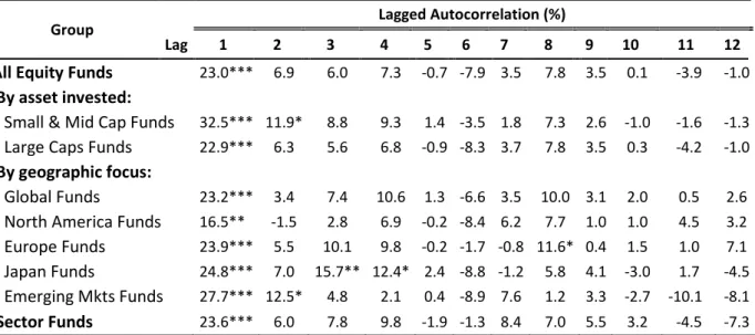
Table III
Return Persistence – Lagged Autocorrelation
This table presents return persistence for each fund category. Study period is between July 1991 and December 2010. The lagged autocorrelation for each group was calculated: where
is the correlation coefficient between variables, the return at and , the k-lagged return. Results
are presented for 1 to 12 lags with each lag being a month. The symbols ***, ** and * denote the statistical significance of the coefficient at 1%, 5% and 10% significance level respectively.
Group Lagged Autocorrelation (%)
Lag 1 2 3 4 5 6 7 8 9 10 11 12 All Equity Funds 23.0*** 6.9 6.0 7.3 -0.7 -7.9 3.5 7.8 3.5 0.1 -3.9 -1.0 By asset invested:
Small & Mid Cap Funds 32.5*** 11.9* 8.8 9.3 1.4 -3.5 1.8 7.3 2.6 -1.0 -1.6 -1.3
Large Caps Funds 22.9*** 6.3 5.6 6.8 -0.9 -8.3 3.7 7.8 3.5 0.3 -4.2 -1.0 By geographic focus:
Global Funds 23.2*** 3.4 7.4 10.6 1.3 -6.6 3.5 10.0 3.1 2.0 0.5 2.6
North America Funds 16.5** -1.5 2.8 6.9 -0.2 -8.4 6.2 7.7 1.0 1.0 4.5 3.2
Europe Funds 23.9*** 5.5 10.1 9.8 -0.2 -1.7 -0.8 11.6* 0.4 1.5 1.0 7.1
Japan Funds 24.8*** 7.0 15.7** 12.4* 2.4 -8.8 -1.2 5.8 4.1 -3.0 1.7 -4.5
Emerging Mkts Funds 27.7*** 12.5* 4.8 2.1 0.4 -8.9 7.6 1.2 3.3 -2.7 -10.1 -8.1 Sector Funds 23.6*** 6.0 7.8 9.8 -1.9 -1.3 8.4 7.0 5.5 3.2 -4.5 -7.3
Table III presents the results for the 1 to 12 months lagged autocorrelations for each one of the 9 mutual fund categories. As can be seen the one-month lag is consistently higher than the other lags and statistical significant, meaning that the t-1 month has a significant explanatory power over the month t. This is also supported by the fact that from all funds more than 46% present statistical significant 1-month serial correlation.5
Other lags do not present systematical significant autocorrelation across all samples, even-though it is noticeable in table III that in some of the fund categories the lags 2 to 4 present some explanatory power, being in some cases statistically significant. All in all, it can be
11
Jul-91 Jan-92 Jul-92 Jan-93 Jul-91 Oct-91 Jan-92 Apr-92 Jul-92 Jul-91 Oct-91 Jan-92 Apr-92 Jul-92 Feb-92
6-months 3-months
R1 Reb. R2 Reb. … R1 R2 ...
Invest Invest Invest
Rebalance Rebalance Rebalance
Rebalance
… …
3-month EsP; 6-month ReF
Est. Period Est. Period Est. Period R1 R2 Estimation Period Estimation Period Estimation Period
6-month EsP; 3-month ReF 6-month EsP; 6-month ReF
Estimation Period Estimation Period Estimation Period 6-months ... ... Rebalance Rebalance
registered the existence of short termed positive autocorrelation being a forewarning for mutual fund return persistency.
2.3 Strategy Methodology
The investment strategy introduced by this thesis is an out of sample (OOS) approach inspired in the momentum anomaly presented by Jegadeesh and Titman (1993). In this ex-ante “hot hands” strategy different estimation periods (EsP) were set – 3 and 6 months, 1, 3 and 5 years – and the rebalancing frequency (ReF) was also tested for different time lags – 1, 3 and 6 months and 1 year. To be included in the estimation rank, funds must present returns during the entire estimation period, mitigating selection biases in newly operating funds. For each one of the 9 categories (e.g. Emerging Markets Funds) 20 different combinations of estimation and rebalancing periods were achieved, producing thus 20 different strategies (e.g. 3-year estimation period rebalancing every month, or 6-month estimation period rebalancing once a year). The strategy is an out of sample (OOS) investment strategy that invests in the top decile funds of the estimation period raw returns’ rank. At the end of each rebalancing frequency the portfolio is rebalanced, i.e. the positions in all funds are sold and new funds will be bought according to the newly estimated top decile.
Figure 1 provides three examples that illustrate the modus operandi of the strategy. On the left panel estimation is completed with six months, and then the investment decision is made. After 6 months (rebalancing frequency) a new investment decision is taken according to the 6-previous-months ranked raw returns estimation, and so forth. For the Figure 1: Strategy Diagrams
12
other two examples the method is the same with different estimation and rebalancing periods. As can be seen above, the estimation periods are non-overlapping except when the estimation period is greater than the rebalancing frequency. It is also important to notice that when the rebalancing frequency is larger than the estimation period not all the monthly raw returns “information” between rebalancing occasions will be included in the estimation period. As it can be seen later, there is some indication that this fact may have a negative impact on the strategy’s performance.
It is important to stress that the investment timeframe starts at October 1991 given that by combining the shortest estimation period (3 months) and the shortest rebalancing frequency (1 month) the first return on the strategy is October 1991’s (4 months after July 1991). Likewise a strategy that estimates and rebalances in 3-month periods has its first return in December, and so on. Moreover, it is vital to emphasize that this strategy operates solely with the information available up to the time of each investment decision. Therefore it has no “knowledge” whether funds will cease operations during next investment period. Thus, it was assumed that if the strategy is invested in a fund that ceases operations the return between that moment and the next rebalancing period is zero. Meaning that if a strategy rebalancing every 6 months invests in a fund that “dies” 3 months later, it is assumed that the return of that fund for the remaining 3 months will be zero. This assumption is quite realistic since (1) liquidating mutual funds are normally able to reimburse investors at fair value, (2) and when funds liquidate is usually due to bad performance, thus the loss of the investor is already accounted in the negative returns preceding the closure date. The performance of the strategies was evaluated by equations (1), (3) and (4) – annualized Sharpe ratio, certainty equivalent of a power utility function and the Carhart’s 4-Factor alphas – three distinct risk adjusted measures.
13
III.
Results
In this section the results of the investment strategy will be presented. These results reflect the different combinations of estimation and rebalancing periods applied to each one of the 9 fund categories. Moreover, this section will be divided in two major parts; the first shows the strategy results in each fund cluster, in the second a thorough analysis on the invested funds portfolio was performed illustrating invested funds’ turnover and specific features of the fund portfolio composition.
3.1 Strategy Results
The performance of the investment strategy is presented through different measures, three of them risk adjusted. Thus the attained returns can be enhanced in risk adjusted terms accounting thus for the risk-return combination that the investor is exposed to. Table IV presents the results of the 20 different strategies for each one of the 9 fund categories. The first and second columns denote each of the 9 fund categories and the different estimation periods, respectively. For each one of the rebalancing frequencies (1, 3 and 6 months and 1 year) four different measures are presented; is the annualized compounded return of the strategy, i.e. return in the investors point of view. The annualized Sharpe ratio (SR) and the annualized certainty equivalent (CE) are two measures that evaluate differently the risk/return relation. Finally the Carhart’s alpha is presented has a measure of selection skill presenting the abnormal returns over passive benchmarks. While looking at table IV’s results one should bear in mind that the OOS testing was performed from October 1991 until December 2010 being this period marked by two recessions (dot-com bubble in 2000 and 2007´s housing bubble). Moreover, and as a background comparison one should be aware that during this period indexes such has the S&P 500 and the MSCI World Index yielded respectively; annualized compounded returns of 8.5% and 6.3%; annualized Sharpe ratios of 0.40 and 0.26; annualized certainty equivalents of 7.4% and 5.3%.
14 Table IV
Strategy Results Summary
This table presents summary results for the strategies performed in each fund category. Data respects the period from July 1991 to December 2010. The first column refers to the results to each one of the 9 categories, the estimation period is the “study” period used to each investment decision. Rebalancing periods are the frequency to each the strategy will be performed, thus the investor portfolio of funds rebalanced. The is the annualized compounded return of the strategy in percentage; SR is the annualized Sharpe Ratio, i.e. the amount of excess return per each unit of risk. The CE is the annualized certainty equivalent, a measure of amount of riskless return (percentage) calculated through the power utility function. Finally α corresponds to the annualized Carhart's 4-Factor alpha (percentage). The symbols ***, ** and * denote the statistical significance of the coefficient at 1%, 5% and 10% significance level respectively. Different statistics provide different strategy result consistency. The darker are the results presented the greater is the certainty of statistical significant of positive achieved results.
Group Estimation Period
1-month Rebalancing 3-month Rebalancing 6-month Rebalancing 1-year Rebalancing
(%) SR CE(%) An. α(%) (%) SR CE(%) An. α(%) (%) SR CE(%) An. α(%) (%) SR CE(%) An. α(%)
All Equity Funds 3 M 19.2*** 0.70*** 17.3 12.6*** 14.2*** 0.55** 11.2 9.2** 14.5*** 0.54** 11.3 11.5** 9.8*** 0.36 6.1 3.4 6 M 17.3*** 0.61** 15.3 8.8*** 15.1*** 0.59** 12.3 8.0* 14.2*** 0.54** 11.4 3.6 10.0** 0.35 4.7 -2.8 1 Y 18.2*** 0.63** 16.1 8.9*** 15.0*** 0.57** 11.9 6.6 11.8*** 0.44* 8.4 -0.7 9.7*** 0.43* 7.8 2.3 3 Y 11.1*** 0.36 8.8 6.1** 10.3*** 0.40 7.3 4.2 9.1*** 0.37 5.8 0.5 9.5** 0.40 7.4 3.3 5 Y 8.9*** 0.28 6.4 4.5 8.4*** 0.32 4.8 4.9 7.9*** 0.31 3.7 3.0 6.3* 0.24 3.7 2.4 Small & Mid Cap Funds 3 M 23.1*** 0.70*** 20.4 16.6*** 15.0*** 0.51** 11.0 13.8** 15.1*** 0.45* 9.9 20.7** 9.4 0.26 3.8 17.1 6 M 19.7*** 0.58** 17.0 12.4*** 13.8*** 0.47* 9.9 9.8 7.3** 0.25 3.3 1.5 5.2 0.19 -0.6 14.9 1 Y 16.4*** 0.48** 13.7 7.6* 14.3*** 0.47* 10.3 8.3 10.5*** 0.35 6.2 1.4 8.6*** 0.34 6.1 0.7 3 Y 6.8*** 0.19 4.5 1.5 6.1*** 0.30 3.0 -1.3 5.1** 0.20 1.4 -4.4 9.2*** 0.35 6.6 5.7 5 Y 4.3*** 0.11 1.9 1.5 2.2 0.14 -1.4 0.1 2.0 0.08 -1.7 -3.2 1.6 0.08 -2.5 0.7 Large Cap Funds 3 M 18.5*** 0.68*** 16.6 12.0*** 13.9*** 0.54** 10.9 8.6* 14.5*** 0.55** 11.4 10.6** 10.5*** 0.38* 6.9 3.6 6 M 17.0*** 0.60** 15.1 8.4** 15.2*** 0.59** 12.4 7.9 14.8*** 0.57** 11.9 3.7 10.5** 0.37 5.1 -4.6 1 Y 18.1*** 0.64** 16.0 8.6*** 14.9*** 0.57** 11.8 6.1 12.1*** 0.45* 8.7 -0.5 7.2*** 0.29 5.5 2.6 3 Y 11.8*** 0.39* 9.5 6.7** 11.2*** 0.43* 8.1 4.9 9.7*** 0.40 6.3 1.4 10.0*** 0.42* 7.9 3.5 5 Y 9.5*** 0.29 7.0 4.9* 9.0*** 0.34 5.5 5.3* 8.6*** 0.34 4.4 3.5 7.1** 0.27 4.5 2.8 Global Funds 3 M 10.1*** 0.38 8.9 4.5** 8.7*** 0.37 7.0 4.3 8.8*** 0.34 6.7 3.7 6.1*** 0.24 4.3 1.2 6 M 9.5*** 0.37 8.4 2.8 9.6*** 0.43* 8.1 4.3 10.5*** 0.51** 9.3 2.4 6.9** 0.27 4.4 -2.5 1 Y 11.3*** 0.46* 10.1 4.6** 9.9*** 0.44* 8.4 4.3* 8.8*** 0.40* 7.3 1.4 6.9*** 0.29 5.3 1.1 3 Y 5.9*** 0.18 4.6 1.1 6.3*** 0.25 4.5 1.5 6.0*** 0.24 4.2 -1.6 5.7** 0.22 4.0 -0.1 5 Y 5.1*** 0.15 3.8 0.5 4.7*** 0.16 2.8 -0.1 4.0** 0.13 2.1 -3.4* 4.8* 0.17 2.9 -0.9
15 Table IV – Continued
Group Estimation Period
1-month Rebalancing 3-month Rebalancing 6-month Rebalancing 1-year Rebalancing
(%) SR CE(%) An. α(%) (%) SR CE(%) An. α(%) (%) SR CE(%) An. α(%) (%) SR CE(%) An. α(%)
North America Funds 3 M 11.0*** 0.45* 9.6 5.5** 11.2*** 0.48** 9.2 7.7** 12.1*** 0.46* 9.5 4.8 9.2*** 0.34 6.9 4.8 6 M 10.6*** 0.44* 9.3 3.8 11.5*** 0.52** 9.9 6.8** 11.1*** 0.52** 9.4 5.1 9.6*** 0.40* 7.1 8.8 1 Y 12.2*** 0.50** 10.7 5.4** 12.8*** 0.54** 10.8 7.4** 12.5*** 0.56** 10.5 7.7* 12.9*** 0.52** 10.6 9.1* 3 Y 9.3*** 0.35 7.6 5.7*** 9.1*** 0.37 6.7 5.9** 8.9*** 0.39 6.9 4.5 8.1*** 0.33 5.9 4.8 5 Y 7.1*** 0.25 5.5 4.0* 6.8*** 0.26 4.5 4.2 5.8*** 0.23 3.8 3.5 4.6 0.16 2.4 1.8 Europe Funds 3 M 12.8*** 0.48** 11.2 5.9** 11.1*** 0.44* 8.5 5.8 12.1*** 0.44* 9.1 6.3 9.2*** 0.36 6.5 5.7 6 M 14.6*** 0.57** 13.0 7.3** 14.5*** 0.59** 12.1 7.8** 14.4*** 0.63** 12.2 5.1 11.4*** 0.51** 9.0 -2.1 1 Y 14.6*** 0.54** 12.8 7.4** 14.0*** 0.54** 11.3 7.6** 12.4*** 0.57** 10.4 2.1 11.3*** 0.47* 8.8 2.1 3 Y 9.8*** 0.35 8.0 5.1* 9.8*** 0.38 7.0 3.4 9.7*** 0.39 6.9 -0.6 10.0*** 0.39 7.1 2.4 5 Y 8.0*** 0.26 5.8 5.0 7.4*** 0.28 3.9 2.4 6.9*** 0.27 3.4 -1.4 6.7* 0.25 3.1 0.4 Japan Funds 3 M 4.4*** 0.10 1.9 -0.6 4.4** 0.19 0.9 2.0 8.3** 0.27 4.2 12.9 5.1 0.17 0.9 10.5 6 M 3.4*** 0.07 1.1 -2.5 2.6 0.14 -0.7 -2.8 0.9 0.07 -3.6 -4.9 1.4 0.11 -4.8 19.0 1 Y 6.5*** 0.16 3.9 -0.8 6.5*** 0.24 3.0 1.3 4.6 0.18 -0.3 -0.3 0.2 -0.04 -2.0 -0.7 3 Y -0.4 -0.03 -3.0 -5.5 -2.1 0.01 -5.4 -6.9 -3.2 -0.06 -7.8 -10.1 -2.4 -0.09 -5.5 -2.7 5 Y 1.3 0.02 -1.5 -3.1 -1.7 0.03 -5.5 -6.4 -5.7* -0.14 -10.3 -13.2 -2.4 -0.05 -5.6 -0.6 Emerging Markets Funds 3 M 18.0*** 0.58** 15.0 11.2** 13.4*** 0.46* 8.2 6.7 16.0*** 0.52** 10.4 9.9 14.8*** 0.45** 7.2 8.9 6 M 17.2*** 0.53** 14.0 7.8* 15.2*** 0.50** 10.0 8.1 17.8*** 0.54** 10.4 8.9 14.1** 0.41* 4.8 -2.8 1 Y 18.0*** 0.56** 14.5 8.0* 14.9*** 0.49** 9.5 3.7 12.2*** 0.40 3.8 0.0 9.2** 0.34 4.3 -1.8 3 Y 9.7*** 0.31 5.9 3.7 8.2*** 0.31 3.6 2.6 4.7 0.21 -1.7 -2.5 4.1 0.17 -0.6 -0.7 5 Y 6.4*** 0.14 2.8 1.4 6.8*** 0.26 1.9 3.8 7.2** 0.29 0.2 4.7 6.0 0.26 -0.4 4.6 Sector Funds 3 M 19.4*** 0.73*** 16.3 13.4*** 17.1*** 0.61** 13.6 11.1** 14.4*** 0.48** 10.5 8.4 10.2** 0.32 5.6 1.4 6 M 21.9*** 0.84*** 19.0 15.1*** 21.5*** 0.73*** 17.8 14.7** 19.2*** 0.54** 13.5 5.9 15.0*** 0.52** 10.5 9.1 1 Y 24.3*** 0.89*** 20.9 14.4*** 20.8*** 0.65** 16.0 12.4* 20.5*** 0.57** 14.7 7.6 14.5** 0.37 9.7 13.1 3 Y 6.0*** 0.22 2.5 6.6 7.3*** 0.27 2.7 7.9* 7.3*** 0.28 2.3 7.5 8.8** 0.34 3.2 11.8** 5 Y 8.4*** 0.31 4.8 9.5** 7.5*** 0.28 2.6 12.7*** 6.3* 0.25 0.7 9.9 2.4 0.13 -3.3 11.1
16
The results illustrated by table IV support the existence of mutual fund performance persistence, suggesting the existence of mutual fund manager’s skill. Moreover the strength of these results reinforces the argument that profitable investment strategies can be constructed exploiting thus this return persistence. As can be seen in table IV these results are quite robust with many performance measures being statistical significant at 10%, 5% and even 1% significance levels. Looking at the results of all the samples it is clear that short term estimation periods yield higher returns than the longer ones. Additionally this evidence is combined by the fact that shorter rebalancing frequencies (1 and 3-months) generate better and more consistent positive results than the longer ones (6-months and 1-year). This evidence is coherent with the findings of several authors namely Grinblatt and Titman (1989, 1992), Hendricks et al. (1993), Gruber (1996), Zheng (1999), Bollen and Busse (2004), Fortin and Michelson (2010) that through different approaches concluded the short term feature of persistence - estimation periods of at most 1 year. One can easily acknowledge this fact by observing in table IV the darker data figures, which mean positive and more robust returns.
The combination of estimation periods and rebalancing frequencies that present consistently better returns is the 1-year estimation with 1-month rebalance, closely followed by the 3 and 6-month estimation with 1-month rebalance. It is also important to highlight that for the 3-month rebalancing frequency the most consistent estimation periods are 6-month and 1-year, and for the 6-month rebalancing the most reliable estimation period is 6 months.
These results are consistent with those showed by Huij and Verbeek (2007) which for a US mutual fund sample between 1984 and 2003 invested monthly (1-month rebalance frequency) based on 36-month raw returns top decile (3-year estimation period) obtained annualized excess returns of 6.96% (7.4% approximate total return) with a Sharpe Ratio of 0.35 and an annualized Carhat’s α of -1.56%. Moreover the returns of investing monthly (1-month rebalancing) in the top decile of 12-(1-month ranked raw returns (1-year estimation) yielded annualized excess returns of 11.64% (roughly 12% total return) with a Sharpe Ratio of 0.55 and annualized Carhart’s α of 0.48%. These results can be compared with the North America sample in the correspondent estimation and rebalancing periods, being very similar with the exception of the Carhart’s α derived from the fact that world factors were
17
employed in this thesis rather than US ones. Huij and Verbeek (2007) also presented results for a Small Cap Funds subsample investing monthly based on the top decile of 12-month ranked raw returns, with excess returns of 12.72% (total returns of roughly 13%) Sharpe Ratio of 0.59 and annualized Carhart’s α of 1.08%. These results can be just partially compared with the Small & Mid Cap sample presented above since it contains other than US funds and funds invested in middle capitalization stocks. Avramov and Wermers (2006) obtained annual excess return of 8.97% (total return of 8.4% roughly) and Sharpe Ratio of 0.44 from a hot hands strategy that invested between 1980 and 2002 in the top decile funds of a 12-month raw return rank (1-year estimation period) rebalancing the portfolio at the beginning of each year (1-year rebalancing frequency).
Additionally other authors such has Hendricks et al. (1993), Bollen and Busse (2004), Huij and Verbeek (2007), Avramov and Wermers (2006), Busse and Tong (2008) study this hot hands strategy by ranking based on different types of α’s. This approach will not be studied throughout this thesis however it is important to mention that these results seem consistent with those previously achieved, with findings of some monotonic relationship between shorter estimation periods and higher top decile performance - Huij and Verbeek (2007).
3.2 Funds Invested Analysis
So far the focus has been mainly on the performance of different strategies in the various fund groups. However it is important to understand in detail the main characteristics of the portfolio of funds invested. This analysis focus on the turnover across different strategies - estimation and rebalancing period’s combinations. Further, special focus was placed on the type of funds that are chosen over time when the strategy is applied to the sector funds category.
In order to understand the behavior of the invested funds’ portfolio across the different strategies table V reports average fund turnover of this portfolio for each combination of estimation period and rebalancing frequency. The figures presented respect the category that includes all the 5.335 funds. The other fund cluster’s turnover rates are very close to
18
the one presented, being this a fair overall estimate. Each number states the average percentage of funds that is changed in each rebalancing event. Meaning that the smaller is turnover, the greater is the percentage of funds remaining in the portfolio i.e., less funds are bought and sold.
Table V Portfolio Turnover
This table presents invested funds’ portfolio turnover for each estimation period and rebalancing frequency combination. Each number states the average percentage of funds that is changed at each rebalancing event.
Rebalancing Frequency
Estimation Period 1 month 3 months 6 months 1 year 3 months 47.8% 79.7% 83.3% 84.3% 6 months 32.8% 58.4% 79.5% 85.4% 1 year 22.4% 41.0% 59.2% 82.3% 3 years 13.1% 24.8% 37.8% 55.4% 5 years 13.9% 22.1% 34.6% 52.3%
Results presented in table V present a clear monotonic trend. Larger rebalance frequencies imply higher fund turnover, whereas larger estimation periods entail lower fund turnover. The economic explanation of these results is very straightforward; larger rebalancing frequencies imply that the portfolio is updated less often. As a result more time will pass between rebalancing events thus, greater amount of new information (raw returns track record) is used in the next rebalancing decision that was not available in the previous one. Therefore a greater fund turnover reflects this “information change” that produces larger changes on the composition of the portfolio. The same reasoning can be applied to the estimation period; the greater the estimation period is more monthly observations will be included in the raw return rank. Therefore at each rebalancing event the weight of new information is lower, meaning that fewer changes in the portfolio will occur.
Two examples will help clarifying this reasoning; for the 3-month estimation and 6-month rebalancing strategy, it is expected to have a very high fund turnover since the rebalancing decision is made upon the 3-previous-month raw return rank thus, at each rebalancing decision (every six months) the information used will be completely different to the one used in the previous rebalance decision. Now instead of 3-months the estimation period is 5 years, when rebalancing every 6 months the weight of new information in the raw
19
returns rank is much lower This implies that the next rebalancing decision will be taken based on the latest 6 month return track records and the remaining 4.5 years were the same used in the previous rebalancing event. Therefore it is expected the fund turnover to be much lower.
Further a more descriptive analysis on the funds invested throughout time is presented. The fund category chosen to perform this analysis requires a quite heterogeneous set of funds. A reasonable approach would be to analyze the category with all funds however, due to the large amount of invested funds per period (over 400 in some periods) the results are not easily comprehensible neither representative. Therefore the focus will be placed on the sector funds category. This group contains funds from many different sectors, such as natural resources, financials, telecommunications, information technology and several others.
In the beginning of the analysis (end of 1991 and 1992) it was clear the predominance in the invested funds’ portfolio of natural resources funds and an increasingly noticeable presence of telecom and information technology funds. In the late 1990’s information technology and pharmaceutical/biotechnology funds dominated the portfolio reflecting the great growth prospects that these sectors witnessed during this period. In the beginning of 2001 it was clear the quick shift to natural resources and real estate funds, traducing the dot-com bubble burst and the comeback to long-established sectors. Throughout the 2000´s until 2006 the sectors invested change in “waves”, after the crash and panic some information technology and telecommunication funds were back among the best performers, then natural resources, real estate and some consumer goods funds were also top-performers. In 2006 and 2007 it was clear the large weight of real estate funds in the portfolio, vanishing right after May 2007 when natural resources funds took dominant position once again. Since then until December 2010 the sectors that have been most invested are natural resources and pharmaceutical/biotechnology funds.
20 0 0.2 0.4 0.6 0.8 1 1.2
Jan-08 Abr-08 Jul-08 Out-08 Jan-09 Abr-09 Jul-09 Out-09 Jan-10 Abr-10 Jul-10 Out-10
C um ul at iv e R e tur n (I nde x)
Sector Funds 1-month Rebalancing Strategies vs. Buy and Hold Strategy (January 2008 - December 2010)
MSCI World 3M Est - 1M Reb 6M Est - 1M Reb 1Y Est - 1M Reb 3Y Est - 1M Reb 5Y Est - 1M Reb
Figure 2 shows several 1-month rebalancing strategies from the sector funds category during a short period of time – January 2008 to December 2010. This short investment timeline supports the conclusion that by allowing the portfolio to update frequently (based on shorter estimation periods) the strategy is able to “ride the wave” of the best funds at each point in time being more importantly capable of quickly adapt the holdings according to changes in market conditions that change the best performing sectors. This fact can be seen in figure 2 where a sudden crash occurs (2008), and the strategies with short and mid-term estimation periods are able to adapt fast, thus performing alike or better than the benchmark. The fact that the sector funds’ category contains very specific pro and anti-cyclical funds is one possible explanation for the fact that this was the group where the implemented strategies yielded the best results.
IV.
Robustness
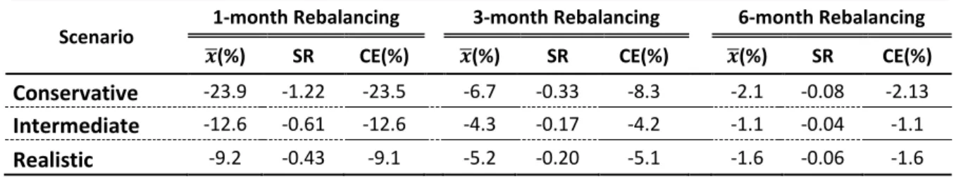
This section tests the robustness of the results achieved with this investment strategy. Returns were tested in expansion vs. recession periods providing a comprehensive knowledge on the strategy’s behavior in different market conditions. Further the results were compared adopting a “buy-and-hold” perspective against the passive benchmark and over different time periods. Additionally the results were tested against transaction costs and the application of this investment strategy to private investors discussed.
21 4.1 Strategy in expansion vs. recession periods
The robustness of the results obtained was tested in different market conditions, i.e. expansion and recession periods. The characterization of these periods was taken from National Bureau of Economic Research, and respects the US economy.6 Small discrepancies may arise has the delimitation of expansion and recession periods is likely to change in other geographic locations. However considering the importance of the US economy in the global markets and aiming for coherence across the analysis this assumption is highly reasonable.7 The expansion periods considered are: form October 1991 to March 2001, from December 2001 to December 2007 and between July 2009 and December 2010. The recession periods are from April 2001 to November 2001 and between January 2008 and June 2009. The calculation of the strategy’s returns in each economic cycle was executed by concatenating expansion and recession periods’ returns separately, generating two continuous time series from which several statistics were computed.
Tables VI and VII illustrate the strategy results for the different fund categories in expansion and recession periods respectively. Each category of funds generates a total of 20 results in both expansive and recessive markets resulting from the 20 different combinations of estimation and rebalancing periods. From these 20 outcomes tables VI and VII present the minimum, maximum and median average annualized return, Sharpe ratio and certainty equivalent. The same performance measures for the aggregate returns of each fund category were also presented, allowing for comparison between strategy and category’s average performance.
6
See http://www.nber.org/cycles.html.
7
Exception is Japan which faced severe recession through the 1990’s, however for the sake of uniformity expansion and recession periods in this analysis are the same as the other samples.
22 Table VI
Strategy Performance Test: Expansion Periods
This table presents strategy results solely in expansion periods between October 1991 and December 2010. For each fund cluster the results from the 20 different strategies were tested in expansion periods. The characterization of these periods was taken from National Bureau of Economic Research. The expansion periods are; October 1991 to March 2001, December 2001 to December 2007 and July 2009 to December 2010. This analysis generated 20 different results in each group of funds. From them, the minimum, maximum and median average annualized return ( , Sharpe ratio (SR) and certainty equivalent (CE) are presented. The section on the right illustrates the EW aggregate performance of the respective fund category in expansion periods.
Group
Strategies in Expansion Periods
EW Group Returns in
Expansion Periods
Min. Median Max.
(%) SR CE(%) (%) SR CE(%) (%) SR CE(%)
(%) SR CE(%)
All Equity Funds 15.9 0.58 12.6 20.2 0.81 16.0 23.4 1.09 21.8
11.3 0.60 10.0
By asset invested:
Small & Mid Cap Funds 11.5 0.27 4.0 17.5 0.53 12.5 27.9 1.14 26.5
12.9 0.67 11.4
Large Caps Funds 13.4 0.61 11.0 20.4 0.80 16.8 23.2 1.05 21.6
11.1 0.59 9.8
By geographic focus:
Global Funds 11.7 0.50 9.7 13.4 0.69 11.8 15.5 0.88 14.5
9.6 0.53 8.5
North America Funds 13.4 0.58 11.2 16.3 0.80 14.2 20.6 0.95 17.6
11.5 0.63 10.2 Europe Funds 17.0 0.63 13.2 19.2 0.85 16.2 21.4 1.11 19.7 12.5 0.67 11.2 Japan Funds 2.9 -0.01 -7.1 9.2 0.19 2.2 17.9 0.40 9.4 3.5 0.01 0.5 Emerging Mkts Funds 11.5 0.29 2.5 22.5 0.60 14.4 29.7 0.95 22.0 15.9 0.67 13.1 Sector Funds 14.1 0.32 3.4 23.7 0.63 16.6 32.6 1.12 28.0 11.6 0.58 10.0
In expansion markets the investment strategy has an outstanding behavior by outperforming significantly the respective fund category’s average. The outperformance within each fund cluster ranged between 40 and 100 percent, meaning that from the 20 different strategy results of each cluster a minimum of 8 outperformed the respective category’s average, being this figure higher in other clusters reaching 100 percent in the large cap funds category. Overall the outperformance is between 79 percent in risk-adjusted measures (SR and CE) and 95 percent in raw returns. These figures indicate that from the overall 180 strategy results (20 in each fund category) 79 percent of them outperform the respective benchmarks in risk-adjusted terms. Further it is noticeable that the 1-month rebalancing strategies with estimation periods of 3, 6 and 12 months are persistently among the best outperformers, being them closely followed by the 6-month estimation and rebalancing periods’ strategy. With respect to the underperforming strategies it is possible to infer that those with longer estimation periods (3 and 5 years) account for more than 2/3 of the total underperformance occurrences.
23 Table VII
Strategy Performance Test: Recession Periods
This table presents strategy results solely in recession periods between October 1991 and December 2010. For each fund cluster the results from the 20 different strategies were tested in recession periods. The characterization of these periods was taken from National Bureau of Economic Research. The recession periods are from April 2001 to November 2001 and between January 2008 and June 2009. This analysis generated 20 different results in each group of funds. From them, the minimum, maximum and median average annualized return ( , Sharpe ratio (SR) and certainty equivalent (CE) are presented. The section on the right illustrates the EW aggregate performance of the respective fund category in expansion periods.
Group
Strategy in Recession Periods EW Group Returns Min. Median Max. Recession
(%) SR CE(%) (%) SR CE(%) (%) SR CE(%)
(%) SR CE(%)
All Equity Funds -28.0 -10.64 -34.6 -19.6 -0.95 -25.2 -8.8 -0.55 -12.6
-19.2 -0.92 -22.5
By asset invested:
Small & Mid Cap Funds -41.9 -7.78 -38.1 -19.8 -0.95 -23.9 -10.7 -0.45 -17.7
-21.0 -0.91 -24.8
Large Caps Funds -27.5 -10.12 -34.2 -19.4 -0.91 -25.2 8.6 -0.55 -12.4
-19.1 -0.92 -22.4
By geographic focus:
Global Funds -27.8 -5.82 -28.4 -20.6 -1.27 -21.9 -10.6 -0.51 -15.3
-20.3 -1.04 -22.6
North America Funds -27.6 -3.93 -27.5 -18.9 -1.05 -21.2 -8.2 -0.39 -15.9
-17.3 -0.87 -20.6 Europe Funds -33.3 -4.26 -35.9 -21.6 -1.24 -24.8 -12.0 -0.54 -18.6 -24.7 -1.16 -26.6 Japan Funds -31.4 -14.79 -29.0 -20.3 -1.20 -23.1 -12.5 -0.87 -13.5 -24.1 -1.20 -25.7 Emerging Mkts Funds -41.7 -4.59 -40.6 -16.9 -0.53 -28.7 -3.0 -0.13 -13.0 -17.6 -0.62 -25.6 Sector Funds -27.6 -2.53 -36.1 -19.0 -0.80 -24.0 -10.5 -0.51 -13.6 -16.6 -0.79 -20.7
In recessive periods the ability of the strategy to outperform the respective benchmark is more limited. The outperformance within each fund cluster remained between roughly 20 and 85 percent, meaning that from the 20 different strategy results of each cluster a minimum of only 3 outperformed the respective category’s average, being this figure higher in other clusters reaching almost 85 percent in the Japan funds category. Comparing with the expanding markets figures, the outperformance in recession periods reduced significantly to around 50 percent in both risk-adjusted (SR and CE) and non-risk adjusted measures (raw returns).
These figures point out that from the overall 180 strategy results (20 in each fund category) solely half of them are able to outperform the respective benchmarks. Additionally, the strategies with 3-month estimation and 1 and 3-month rebalancing and the one with 6-month estimation and 12-6-month rebalancing are the ones that more often are able to better outperform the category’s average in recession periods. This induces to conclude
24
that in falling markets the best strategy is to look at short term performance and adapt the portfolio frequently. The 6-month estimation and 12-month rebalancing strategy does not undermine the previous conclusion rather suggests the existence of some sort of longer term superior quality in some funds supported by frequent outperformance of strategies 3 and 5-year estimation periods and 3-month rebalancing frequencies.
The strategies that underperformed the most in recession periods were those with less frequent rebalancing (1 year) and with extreme estimation periods (3 months, 3 and 5 years) and also the strategy with 3-month estimation and 6-month rebalance frequency. It seems clear that in recessive markets the worst performers are those that adapt less frequently the invested funds’ portfolio and those that estimate very shortly and hold their portfolio for a consider amount of time. This suggests that the information loss that occurs when rebalancing period is greater than the estimation one has a major negative impact when this difference is significant and in a recessive market context. Additionally, during these recession periods if one had invested in the bottom decile instead of the top one the results would become much more extreme, the number of outperforming strategies would remain roughly the same but the scale of the underperformers would be much wider. All in all, it suggests that this investment strategy possesses some fund selection skill, even in declining markets.
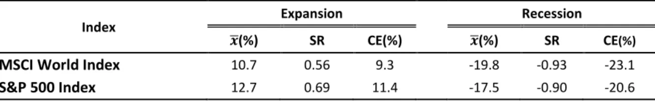
Table VIII
Index Performance: Expansion and Recession Periods
This table presents the performance of the MSCI World and S&P 500 Indexes between October 1991 and December 2010. The performance of each stock index during expansion and recession periods is presented. The characterization of these periods was taken from National Bureau of Economic Research. The expansion periods are; October 1991 to March 2001, December 2001 to December 2007 and July 2009 to December 2010 and the recession periods are from April 2001 to November 2001 and between January 2008 and June 2009. Mean annualized return ( , Sharpe ratio (SR) and certainty equivalent (CE) are presented in each period respective to each index.
Index Expansion Recession
(%) SR CE(%) (%) SR CE(%)
MSCI World Index 10.7 0.56 9.3 -19.8 -0.93 -23.1 S&P 500 Index 12.7 0.69 11.4 -17.5 -0.90 -20.6
25
Table VIII presents the performance of the MSCI World Index and S&P 500 Index during the same expansion and recession periods presented in tables VI and VII. This information allows the comparison between results presented in these tables and worldwide used investment benchmarks. The overall results of each fund category presented in table VI and VII fit quite well with the figures presented from these two indexes (exception is Japan cluster). This means that the conclusions drawn above concerning expansion and recession periods hold for the most part also with respect to these benchmarks. All in all, it can be seen the quality of the strategy that outperforms most of the times in expansion periods, whilst is able to provide outperformance during recession ones.
4.2 Strategy vs. Buy and Hold
A common practice among industry practitioners is the comparison between the cumulative fund performance since its inception and the return that investor would yield if it was invested through the same period in the comparable passive index. Here the same approach is reproduced, providing an industry-like analysis of the quality of the strategy. Figures 3 and 4 present the behavior of the strategies with 1-month rebalance frequency (and different estimation periods) of the overall fund sample described before as “All Equity Funds”. Figure 3 compares the cumulative returns of the 5 different 1-month rebalancing frequency strategies (estimation periods of 3 and 6 months, 1, 3 and 5 years) with the passive benchmark’s one in the timeframe of the strategy i.e., between October 1991 and December 2010. The choice of having the MSCI World Index as the passive benchmark is reasonable due to the geographic spread of funds included in the sample. Figure 3: Strategy vs. Buy and Hold Index
0 5 10 15 20 25 30 C u m u la ti ve R e tu rn ( In d e x)
All Funds 1-month Rebalancing Strategies vs. Buy and Hold Strategy (MSCI World Index)