Development of Innovative Methodologies for the Treatment of Uncertainties in the Earthquake Loss Estimation of Building Portfolios

(1)

F

ACULDADE DE

E

NGENHARIA DA

U

NIVERSIDADE DO

P

ORTO

DEVELOPMENT OF INNOVATIVE

METHODOLOGIES FOR THE TREATMENT

OF UNCERTAINTIES IN THE EARTHQUAKE

LOSS ESTIMATION OF BUILDING

PORTFOLIOS

Luis Miguel Costa Sousa

Doctoral Program in Civil Engineering

Supervisor: Mário António Lage Alves Marques Co-supervisor: Humberto Salazar Amorim Varum

Co-supervisor: Vitor Emanuel Marta da Silva

(2)

(3)

F

ACULDADE DE

E

NGENHARIA DA

U

NIVERSIDADE DO

P

ORTO

DEVELOPMENT OF INNOVATIVE

METHODOLOGIES FOR THE

TREATMENT OF UNCERTAINTIES

IN THE EARTHQUAKE LOSS

ESTIMATION OF BUILDING

PORTFOLIOS

A thesis submitted to the Faculty of Engineering of the

University of Porto in fulfilment of the requirements for

the degree of Doctor of Philosophy

Scientific coordination of Dr. Mário António Lage Alves Marques,

post-doctoral researcher at the Faculty of Engineering of the University of Porto;

with co-supervision of Professor Humberto Salazar Amorim Varum, full

professor at the Faculty of Engineering of the University of Porto, and Dr.

Vitor Emanuel Marta da Silva, post-doctoral researcher at the Department

of Civil Engineering of the University of Aveiro

Orientação científica do Doutor Mário António Lage Alves Marques,

investigador post-doc da Faculdade de Engenharia da Universidade do

Porto; e coorientação do Professor Doutor Humberto Salazar Amorim

Varum, professor catedrático da Faculdade de Engenharia da Universidade

do Porto, e Doutor Vitor Emanuel Marta da Silva, investigador post-doc do

(4)

(5)

i

Abstract

Earthquake losses registered worldwide over the last century have triggered crippling effects on the economic and social systems of wealthy and undeveloped countries alike. In the face of ever increasing impacts, earthquake loss modelling is essential for the prediction, prevention and mitigation of the adverse effect of future seismic events. Given the complex nature of the process, it is utopian to seek for absolute certainty when gathering the required resources. As an inherent property of any analytical process, uncertainty must not be ‘removed’ from the equation. One must seek to improve our knowledge to the extent imposed by practical limitations. However, a seismic risk assessment can only be meaningful if fully coupled with its accompanying analysis of uncertainty, be that aleatory or knowledge-based.

In the context of seismic risk, several questions remain entirely unanswered or lack a deeper understanding. Therefore, in the present work, important issues related with the treatment of uncertainty in portfolio loss estimation are addressed, focusing on the building exposure and vulnerability counterparts. With regard to building exposure, an innovative algorithm is proposed, providing an automated tool for the development of exposure datasets of industrial buildings in Europe, based on open-access data and Volunteered Geographic Information (VGI). With respect to building fragility and vulnerability, on the other hand, the present work sheds light on several problems and limitations in current practice, focusing on the impact that (commonly assumed) hazard disaggregation approximations have on various risk metrics. Building on the latter findings, the appropriate treatment of structural capacity and seismic demand variability is further addressed. More specifically, questions regarding the treatment of such sources of uncertainty are studied from a statistical significance point of view, providing novel and robust approaches to the problems of hazard-compatible ground motion selection, estimation of building response variability, and representation of uncertainty and (spatial) correlation of damage exceedance probabilities. This contribution is subsequently extended to the definition of building vulnerability, whereby innovative conditional fragility functions and the resulting vulnerability model are proposed and included in a novel loss assessment framework. The proposed methodology allows a robust evaluation of the impact of variability and spatial correlation of building vulnerability, highlighting important limitations of state-of-the-art methods.

The combined contribution of the aforementioned efforts results in the final undertaking of this work, which consists of the development of a methodology that is able to adequately propagate the epistemic uncertainty of hazard modelling into the corresponding risk results. The latter ensures a robust and statistically meaningful representation of aleatory (and epistemic) variability in structural response and damage exceedance probability, as well as the explicit modelling of the (hazard-consistent) spatial correlation of building losses.

(6)

(7)

iii

Resumo

Perdas devidas à acção sísmica registadas a nível global durante o último século têm provocado efeitos devastadores no tecido económico e social de diversos países, mais ou menos desenvolvidos. Perante este impacto, a modelação analítica de perdas sísmica torna-se uma ferramenta essencial para a previsão, prevenção e mitigação do efeito adverso de futuros eventos sísmicos. Dada a incerteza associada a este processo, é utópico pretender obter resultados com absoluta certeza. Como parte inerente de qualquer estudo analítico, a incerteza não deve ser ‘removida’ da equação. O objectivo reside na melhoria do conhecimento associado às diferentes variáveis envolvidas, na medida imposta por limitações de ordem práctica. No entanto, a robustez de um estudo de risco sísmico é garantida apenas quando este é devidamente acompanhado de uma análise das várias incertezas, sejam estas de ordem epistémica ou aleatória.

No âmbito do risco sísmico, várias questões continuam inteiramente sem resposta ou necessitam de um estudo mais aprofundado. Deste modo, vários problemas relacionados com o tratamento da incerteza são abordados neste trabalho, com especial enfase nas components de avaliação do património exposto e sua vulnerabilidade sísmica. No que respeita ao primeiro, é desenvolvido um inovador algoritmo automático para a caracterização da localização espacial de edifícios industriais na Europa, com base em fontes públicos de informação geo-referenciada. No que diz respeito à fragilidade de edifícios, o presente trabalho centra-se em diversas limitações identificadas na literatura, focando-se no impacto que aproximações generalizadamente assumidas durante o precesso de desagregação de perigosidade sísmica têm em diferentes medidas de risco. Com base nestes resultados, o tratamento da variabilidade na resposta estrutural e acção sísmica é subsequentemente abordado. Mais concretamente, as referidas fontes de incerteza são estudadas do ponto de vista estatístico, conduzindo a propostas alternativas e robustas com vista à análise de problemas de: selecção de accelerogramas naturais compatíveis com a perigosidade local, estimativa da variabilidade na resposta estrutural, e representação da incerteza e correlação espacial entre probabilidades de excedencia de dano. Esta contribuíção é ainda extendida à definição de vulnerabilidade, meio pelo qual as propostas funções de fragilidade condicionais são integradas num nova metodologia para a estimativa de perdas. Esta metodologia permite efectuar a avaliação probabilística do impacto da variabilidade e correlação espacial da vulnerabilidade de uma forma robusta, evidenciando limitações importantes no estado da arte.

A conjugação dos esforços acima mencionados resulta no estudo final deste trabalho, que consiste no desenvolvimento de uma metodologia que é capaz de, de forma consistente, ter em conta a incerteza epistemica desde a avaliação de perigosidade até ao cálculo de perdas. É assim possível uma representação da incerteza aleatória (e epistemica) na resposta estrutural e probabilidade de dano, bem como a modelação adequada da correlação espacial de dano sísmico.

(8)

(9)

v

Acknowledgements

I would like to start by expressing my most sincere gratitude to Dr. Mário Marques, my supervisor, for his encouragement, knowledge, and human qualities, constantly present throughout this work. I am deeply grateful for his motivation and wisdom, for his selfless help, and more importantly, his friendship.

To Dr. Vitor Silva, my co-advisor and friend, I would like to express my deepest appreciation for the crucial role in this thesis, particularly for encouraging and enabling me to start this work. His personal, scientific and professional qualities are one of the main drivers of my efforts to achieve increasingly demanding goals.

To Professor Humberto Varum, my co-supervisor, I must extend my admiration and gratitude for the contributions and support that ultimately made this thesis possible.

To Dr. Helen Crowley, Dr. Graeme Weatherill and Dr. Paolo Bazzurro, co-authors in four of the scientific papers developed within the context of this thesis, I would like to express my infinite appreciation for their example, scientific knowledge and invaluable contribution to this work.

My sincere gratitude goes to Dr. Rui Pinho, Professor Gian Michele Calvi and Dr. Ricardo Monteiro, who through their example, energy and leadership have decisively contributed not only for my personal and scientific achievements during the time I spent in Pavia, but also for enabling future prospects.

To Professor Raimundo Delgado, I would like to express my admiration and gratitude for the selfless contribution to this thesis, as well as the decisive influence on making it possible. His example and help throughout this journey are infinitely appreciated.

To my friends in Pavia, namely Romain Sousa, Cecilia Nievas, Jennisie Tipler, James Brown, Vitor Silva, Daniela Rodrigues, Rui Figueiredo and Catarina Costa, I would like express my sincere appreciation for the shared moments of companionship. A special thanks goes to Caterina Manieri, for her kind affection and friendship.

To all my childhood friends, especially José Barbosa, João Azevedo and Hugo Garcês, I am thankful for all the diatribes of nonsensical conversations and laughter that make efforts like this worthwhile.

To my Parents, my amazing brothers, my beautiful sisters, and my joyful nephews and god-daughter, I would like to say a special thank you, for all the love and support.

Finally, I would like to express my deepest admiration and love to Venetia Despotaki. This accomplishment would not exist without the love, patience and warmth of such a beautiful human being.

(10)

(11)

vii

List of Figures

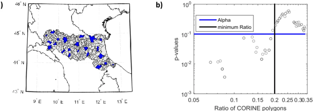
Figure 2.1 – Georeferenced database of non-residential areas (black) provided by the CORINE Land Cover project (CORINE, 2006) for 36 European countries. ... 11 Figure 2.2 – Industrial land use areas provided by the OSM database (blue) for 36 European countries, as of October 2015. ... 12 Figure 2.3 – Schematic representation of the main algorithm workflow ... 13 Figure 2.4 – Schematic representation of the operations performed by the Area Calculator for an example area: a) Inputs: CORINE non-residential area (white) and OSM commercial area (grey), and b) Industrial area output. ... 14 Figure 2.5 – Schematic representation of the operations performed by the Building

Exposure Calculator for an example area: a) Inputs, and b) Building-by-building

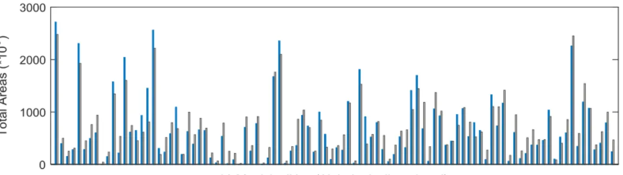
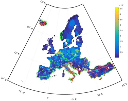
output. ... 14 Figure 2.6 – Schematic representation of the completeness algorithm workflow ... 15 Figure 2.7 – a) Region of Emilia Romagna, Italy (grey), and one simulated set S of 22 administrative boundaries, (blue) randomly selected from the total of 353 municipalities, b) p-values of the B-KS test as a function of the fraction of polygons with complete data ... 17 Figure 2.8 – a) Total industrial built area in Denmark (98 municipalities), as obtained from Statistics Denmark (2015), b) Industrial built area of 18 districts in Portugal, according to PRISE (2013-2015) and Araújo et. al. (2015), and c) industrial built area in Emilia Romagna, Italy (353 municipalities), as obtained from Geoportale Emilia Romagna (2015). ... 19 Figure 2.9 – Bar chart comparing “real” (blue) and predicted values (grey) of total built area of industrial buildings, for 98 municipalities in Denmark... 19 Figure 2.10 – a) Inferred versus “real” values of industrial building built areas for 98 municipalities in Denmark, and b) corresponding ratio between predicted and “real” and values. ... 20 Figure 2.11 – Bar chart comparing real (blue) and predicted values (grey) of total built area of industrial buildings, for 18 districts in Portugal ... 20 Figure 2.12 – a) Inferred versus “real” values of industrial building built areas for 18 districts in Portugal, and b) corresponding ratio between predicted and “real” and values. ... 20 Figure 2.13 – Bar chart comparing “real” (blue) and predicted values (grey) of total built area of industrial buildings, for 10 provinces in the region of Emilia Romagna, Italy ... 21 Figure 2.14 – a) Inferred versus “real” values of industrial building built areas, for 353 municipalities in the region of Emilia Romagna, Italy, and b) corresponding ratio between predicted and “real” and values. ... 21

(16)

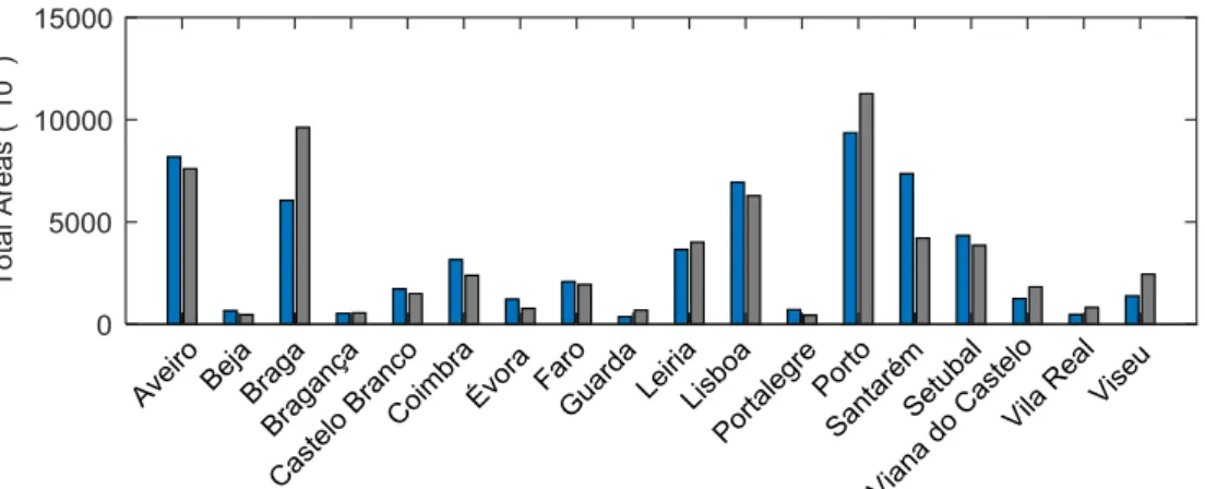
Figure 2.15 – Exposure dataset of industrial building areas (m2_{) developed for 36}

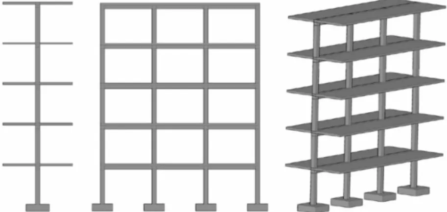
countries in Europe, aggregated at the first administrative level (m2). ... 22 Figure 2.16 – European hazard map of peak ground acceleration (PGA) with 10% exceedance probability in 50 years (in units of g), adapted from SHARE (2015) . 23 Figure 2.17 – Illustration of industrial “exposure at risk” in Europe. The solid contour lines enclose regions where PGA values of 0.05g (green), 0.15g (orange), and 0.30g (red), respectively, are expected to be exceeded with 10% probability in 50 years. ... 23 Figure 2.18 – Total area of industrial assets exposed to PGA of 0.15g (grey) and 0.30g (black) or higher with a mean return period of 475 years. Graph include only the top 10 countries ... 25 Figure 2.19 – Same as in Figure 2.18 but normalized by the total area of industrial buildings in each country. ... 25 Figure 3.1 – Schematic view of the five-story RC frame model: front (left), side (centre) and isometric view (right) without infills, adapted from Silva et. al. (2014). ... 33 Figure 3.2 – Rupture-by-rupture disaggregation (method 1), using the ERF generated for the FSBG-model, and Sa(T1)=0.5g. Ruptures are grouped with ΔMw = 0.2 ΔRjb =5

km, for visual clarity. ... 36 Figure 3.3 – a) Target spectral ordinates of periods ranging between 0.1 and 3.0 seconds (solid lines correspond to the mean and dashed lines represent 16 and 84 percentiles, i.e. mean +/- 1 standard deviation), and b) target cumulative probabilistic distribution functions of HI. In both cases, the results from disaggregation methods 1 and 2a to 2e (FSBG-model, CY08) are illustrated, considering a mid-code structure of 5 floors, for a conditional Sa(T1)=0.5g. ... 40

Figure 3.4 – a) p-values obtained with the KS test, when comparing empirical distributions of Sa(T=0.05 to 3.0 sec.) derived from records selected with approximate target distributions (methods 2a to 2e), as opposed to those obtained with the exact method 1. Conditioning Sa(T1)=0.5g (MC-5), FSBG source model

and AB10 GMPE. b) same as a) but with CY08 GMPE. ... 41 Figure 3.5 – Fragility functions obtained with records selected based on methods 1 and 2a to 2e, for all the combinations of GMPE / source model. Limit state of Collapse using the ISD criteria, C-5 building class. ... 43 Figure 3.6 – Fragility functions obtained with records selected based on methods 1 and 2a to 2e, for all the combinations of GMPE / source model. Limit state of Collapse (GD criteria), C-5 structural typology. ... 44 Figure 3.7 – Disaggregation results for methods 1 and 2c, considering AB10 GMPE and the ERF generated for the AS, FSBG, SEIFA and VF models, for Sa(T1)=0.5g (C-5). Ruptures in the exact method 1 are grouped with ΔMw = 0.1 / ΔRjb =1 km, for

visual clarity, and, in practice, contribution probabilities of method 2c result from aggregation of those of method 1 into coarser M, Rjb intervals. ... 45

(17)

xiii

Figure 3.8 – a) Vulnerability functions obtained with records selected based on methods 1 and 2a to 2e, for AS/AB10 (left) and SEIFA/AB10 (right), combinations. ISD criteria and C-5 structural typology, b) same as a), considering GD criteria. ... 47 Figure 3.9 – a) Uncertainty in the vulnerability model obtained from bootstrapping with replacement from the original sets of damage exceedance probabilities. Structural typology of C-5, methods 2a and 2e, AS/AB10 combination, and ISD criteria, b) same as a), considering GD criteria. ... 48 Figure 3.10 – Probability of ‘Error’ being higher than 10%, where ‘Error’ is the absolute (normalized) difference between: a) AAL obtained from methods 2a to 2e, and b) AAL computed using method 1. Inter-story Drift Criteria. ... 49 Figure 3.11 – Probability of ‘Error’ being higher than 10%, where ‘Error’ is the absolute (normalized) difference between a) AAL obtained from methods 2a to 2e, and b) AAL computed using method 1. Global Drift Criteria. ... 49 Figure 3.12 – Probability of ‘Error’ being higher than 10% obtained with method 2a, for all the combinations of source model / GMPE, structural classes, and limit state criteria. For clarity, horizontal lines correspond to the mean errors of all the structural classes, for each of the different source models. ... 50 Figure 3.13 – Average annual collapse probability (mid-code and post-code buildings) computed using methods 1 and 2a to 2e, for the AS/AB10 combination. ... 52 Figure 4.1 – Schematic view of the five-story RC frame model: front (left), side (centre) and isometric view (right) without infills, adapted from Silva et. al. (2014). ... 58 Figure 4.2 – Evaluation of building response distribution – methodology flowchart. ... 67 Figure 4.3 – BF test statistic (p-value) for 100 synthetic 5 story frames, records selected and scaled to a level of Sa(T1)=1.0g. P-values higher than 0.05 indicate that the null

hypothesis of equal variance cannot be rejected at 5 % significance, for GD (left) and

ISD (right). ... 69

Figure 4.4 – Contribution to hazard determined by disaggregation on M, R, GMPE . For each M, R pair, lower and upper “bars” illustrate the contribution of Atkinson & Boore (2006) and Akkar & Bommer (2010) GMPEs, respectively. Conditional

Sa(T1)=0.5g, for 2 story (left) and 5 story frames (right). ... 70

Figure 4.5 – Target and empirical probabilistic distributions of PGA (left), target 50th, 16th and 84th percentile spectral ordinates between 0.05 sec and 3.0 sec, and selected ground motions (right). Conditioning Sa(T1)=0.5g, for 5 story frames (provided by

selection algorithm, adapted from Bradley (2015)). ... 70 Figure 4.6 – Assessment of scaling robustness of the employed record selection methodology for demand parameters of Global Drift (left) and Inter-story Drift (right). ... 71 Figure 4.7 – P-value of the KS test obtained for each ground motion record, 2 story (left), 5 story (middle) and 8 story (right) classes. P-value higher than 0.05 indicate that the null hypothesis that the sample follows a normal distribution cannot be rejected at a 5 % significance level, for GD and ISD. ... 72

(18)

Figure 4.8 – P-value of the KS test obtained for each synthetically generated frame, 2 story (left), 5 story (middle) and 8 story (right) classes. P-value higher than 0.05 indicate that the null hypothesis that the sample follows a normal distribution cannot be rejected at a 5 % significance level, for GD and ISD. ... 72 Figure 4.9 – Evaluation of uncertainty and correlation in damage exceedance probabilities – methodology flowchart. ... 73 Figure 4.10 – Record-specific distributions of EDP and corresponding probabilities of exceedance of ED, determined according to ISD criteria for 8-story frames. Records selected and scaled for Sa(T1)=1.0g. ... 74

Figure 4.11 – Absolute Error attained when evaluating 600 record-specific probabilities of exceedance (60 ground motions times 10 levels of Sa(T1)) computed as the ratio

between number of exceedances and total number of analysis, as a function of the result obtained through Equation 4.8. Response criteria of ISD, for 2 (left), 5 (middle) and 8 story buildings (right). ... 75 Figure 4.12 – Absolute Error attained when evaluating 600 record-specific probabilities of exceedance computed as the ratio between number of exceedances and total number of analysis, as a function of the result obtained through the methodology presented in this section. Response criteria of GD, for 2 (left), 5 (middle) and 8 story buildings (right). ... 77 Figure 4.13 – Record-specific probabilities of exceedance of SD, MD, ED and Col, as a function of GD (upper) and ISD criteria (lower), for 5-story buildings. ... 78 Figure 4.14 – Empirical probability density - 𝑓[𝑃𝑙𝑠𝑖|𝑆𝑎𝑇1 = 𝑎] - of damage exceedance probability of Extensive Damage and corresponding fitted Beta models, damage criteria of ISD for 5-story frames. ... 79 Figure 4.15 – Record-specific probabilities of exceedance of SD, MD, ED and Col, as a function of GD (upper) and ISD criteria (lower), and corresponding 𝑃𝑙𝑠𝑖|𝑆𝑎𝑇1 = 𝑎 (illustrated by the black squares), for 5-story buildings. ... 80 Figure 4.16 – Empirical probabilistic distributions of aggregated loss computed for a hypothetical portfolio of 100 spatially distributed buildings subjected to

Sa(T1)=0.5g, with zero and full correlation between 𝑓[𝑃𝐶𝑜𝑙. |𝑆𝑎𝑇1 = 0.5𝑔] at each

of the 100 sites. Limit state criteria of GD (left). Beta approximation to 𝑓[𝑃𝐶𝑜𝑙. |𝑆𝑎𝑇1 = 0.5𝑔] (right). Although not presented for the sake of visual clarity, the means of distributions with full and zero correlation are equal, as determined by Equation 4.10, whereas the variability changes proportionally to 𝜌𝑚, 𝑛 (Equation 4.11)... 82 Figure 4.17 – Record-specific probabilities of exceedance of ED, as a function of GD criteria, and corresponding conditional fragility functions for the cases of

Sa(T1)=0.5g, 0.8g and 1.0g, for 5-story buildings ... 82

Figure 4.18 – Most efficient conditional IMi for each structural class and level of Sa(T1).

For each level of Sa(T1), the correspondent IMi (which is also a spectral ordinate) is

represented by the corresponding period of vibration. Fragility assessment in terms of GD (left) and ISD criteria (right). ... 83

(19)

xv

Figure 5.1 – Regression uncertainty of 𝐹𝐶𝑜𝑙𝑙𝑎𝑝𝑠𝑒|𝐼𝑀𝑖, 𝑆𝑎𝑇1 = 0.5𝑔, the Conditional

Fragility Function of Collapse for 5-story frames, given Sa(T1)=0.5g and damage

criteria of GD. For the considered level of Sa(T1), the most efficient IMi is the

spectral acceleration at a period of vibration of 1.89 sec. ... 89 Figure 5.2 – Graphical illustration of the KS test performed when comparing distributions of collapse probability attained through Equation 5.1 (“exact”) and Equation 5.2 (simulated) according to Global Drift criteria for 5 story frames and levels of Sa(T1)

ranging from 0.7g to 1.0g. ... 90 Figure 5.3 – Ratio between KS test statistics and critical value (Dcrit) when comparing distributions of exceedance probability determined based on Equation 1 and Equation 2. Ratios inferior to 1.0 indicate that the null hypothesis that the samples follow identical distributions cannot be rejected at a 10 % significance level, in terms of ISD (left) and GD (right)... 91 Figure 5.4 – Ratio between Schematic representation of the event-based simulation of ground motion fields of Sa(T1). ... 95

Figure 5.5 – Schematic illustration of the generation of S conditional spatially cross-correlated ground motion fields of 𝐼𝑀𝑖|𝑆𝑎𝑇1 = 𝐴 for GMFj and Rupn. ... 96

Figure 5.6 – Schematic representation of simulation of spatially correlated values of 𝐼𝑀𝑖|𝑆𝑎𝑇1 = 𝑎 for GMFj and Rupn, and corresponding damage exceedance matrix.

... 97 Figure 5.7 – Illustration of probabilistic normal distribution of 𝐹𝑙𝑠𝑖|𝐼𝑀𝑖 = 𝑖𝑚𝑖, 𝑆𝑎𝑇1 =

0.5𝑔 for two distinct levels of IMi: imi1 and imi2. Conditional Fragility Functions of

5-story frames given Sa(T1)=0.5g and damage criteria of GD. ... 99

Figure 5.8 – Schematic representation of the damage exceedance matrix resulting from the evaluation of 200 bootstrapped conditional fragility functions at each simulated value of IMi (designated as imi) ... 100

Figure 5.9 – Schematic Schematic representation of the damage matrix resulting from the application of a consequence model to the damage exceedance matrix schematically presented in Figure 5.8. ... 101 Figure 5.10 – Schematic representation of computation of 𝑓𝐿𝑜𝑠𝑠|𝑅𝑢𝑝𝑛, 𝐺𝑀𝐹𝑗, 𝐺𝑀𝑃𝐸𝑚 for a portfolio of buildings of a given Class, distributed across LL sites where Sa(T1)=a. ... 102

Figure 5.11 – Schematic Vulnerability Model of 2, 5 and 8-story buildings characterized by intensity-specific distributions of damage ratio (for the site of Lisbon, Portugal), using the GMPE of Atkinson & Boore (2006). ... 103 Figure 5.12 – Total replacement value (EUR) of two (upper left), five (upper right) and eight-story (bottom) reinforced concrete pre-code buildings located in the district of Lisbon, Portugal. Spatial resolution of 1km2. ... 105 Figure 5.13 – Record-specific probabilities of exceedance of ED, as a function of GD criteria, and corresponding conditional fragility functions for the cases of

(20)

and associated uncertainty determined by 200 bootstrapped lognormal fragility curves, for 5-story buildings... 107 Figure 5.14 – Loss exceedance curves of two, five and eight-story building portfolios, determined using fragility models a and b, derived based GD (upper) and ISD criteria (lower). ... 108 Figure 5.15 – Representation of 𝑃𝑙𝑠𝑖|𝑆𝑎𝑇1 = 𝑎1.0𝑓𝑃𝑙𝑠𝑖|𝑆𝑎𝑇1 = 𝑎𝑑𝑝 (area in blue, referred as ‘cumulative probability’, for simplicity), and corresponding values of 𝑃𝑙𝑠𝑖|𝑆𝑎𝑇1 = 𝑎 (black dashed lines). Damage state of ED and GD criteria, for 5-story frames. “Empirical” and “Fitted Beta” refer, respectively, to the empirical distribution 𝑓[𝑃𝑙𝑠𝑖|𝑆𝑎𝑇1 = 𝑎] and the corresponding fitted Beta model, as proposed in section 4.4.4. ... 109 Figure 6.1 – Tectonic region environment (TRT) associated with each of the sources of the AS-model (left) and the FSBG-model (right). Stable Continental and Active Shallow sources are illustrated as: light and darker blue, respectively, for area sources, and light and darker red, respectively, for fault traces. Dashed circles represent the maximum distance of 250 km... 117 Figure 6.2 – Illustration of the source model / GMPE logic tree adopted for the sites of Faro and Lisbon. Acronyms adopted for each source model / GMPE are presented adjacently. ... 117 Figure 6.3 – Rupture-by-rupture disaggregation considering the ERF generated for the AS-model (left), FSBG -model (middle) and SEIFA-model (right), for PGA=0.5g and site of Lisbon (SCC GMPE of AB10). For visual clarity, ruptures are grouped into M / R bins of 0.2 / 5 km intervals. ... 119 Figure 6.4 – Schematic representation of the five-story RC frame model: front (left), side (centre) and isometric view (right) with infills, adapted from Silva et al. (2015a) 120 Figure 6.5 – Target spectral ordinates of periods ranging between 0.05 and 3.0 seconds (solid lines correspond to the mean and dashed lines represent 16 and 84 percentiles, i.e., mean +/- 1 standard deviation). Sites of Lisbon (upper) and Faro (lower), considering 2, 5 and 8-floor structures and a conditional Sa(T1)=0.5g. ... 122

Figure 6.6 – p-values obtained with the KS test when comparing empirical distributions of HI computed for each of the logic-tree branches applicable to the site of Lisbon. Structural typologies of 2, 5 and 8-floors and conditional Sa(T1)=0.5g. p-values

lower than 0.1 are plotted in black. ... 123 Figure 6.7 – Record-specific distributions of EDP and corresponding probabilities of exceedance of Extensive Damage, determined according to ISD limit state criteria for 8 story frames. Records selected and scaled for Sa(T1)=1.0g (previously

presented as Figure 4.10) ... 124 Figure 6.8 – Record-specific probabilities of exceedance of SD, MD, ED and Col, as a function of GD (upper) and ISD criteria (lower). Site of Lisbon and 5-story buildings (previously presented as Figure 4.13). ... 125

(21)

xvii

Figure 6.9 – KS test performed when comparing distributions of Col. probability conditioned on Sa(T1)=0.5g, at the site of Lisbon. Damage criteria of GD, and

structural classes of 2, 5 and 8-story buildings. ... 126 Figure 6.10 – p-values obtained with the KS test when comparing empirical distributions of damage exceedance probability computed for each of the logic-tree branches applicable to the site of Lisbon. Structural typologies of 2 (left), 5 (middle) and 8-floors (right), conditional Sa(T1)=0.5g, and GD criteria. p-values lower than 0.1 are

plotted in black. ... 127 Figure 6.11 – p-values obtained with the KS test when comparing empirical distributions of damage exceedance probability computed for each of the logic-tree branches applicable to the site of Lisbon. Structural typologies of 2 (upper), 5 (middle) and 8-floors (lower), conditional Sa(T1)=0.5g, and ISD criteria. p-values lower than 0.1 are

plotted in black. ... 128 Figure 6.12 – p-values obtained with the KS test when comparing empirical distributions of damage exceedance probability computed for each of the logic-tree branches applicable to the site of Faro. Structural typologies of 2, 5 and 8-floors, conditional

Sa(T1)=0.5g, and GD criteria. p-values lower than 0.1 are plotted in black, and

branches are numbered from 1 to 60. ... 129 Figure 6.13 – Total replacement value (EUR) of two (left), five (middle) and eight-story (right) reinforced concrete pre-code buildings located in the district of Lisbon, Portugal. Spatial resolution of 1km2 ... 130 Figure 6.14 – Total replacement value (EUR) of two (left), five (middle) and eight-story (right) reinforced concrete pre-code buildings located in the district of Faro, Portugal. Spatial resolution of 1km2. For the sake of visual clarity, only a part of the district is shown. ... 130 Figure 6.15 – Example of a ‘branch-specific’ fragility model and corresponding vulnerability, using the damage-to-loss relationship proposed by Silva et al. (2015a) and the 2-story building class. In this case, branch AS-AB10 and the site of Lisbon are selected, and GD criteria are considered. For simplicity, ‘poE’ stands for ‘probability of exceedance’. ... 132 Figure 6.16 – Loss exceedance curves obtained with models a) and b) for branch

AS-AB10. 5-story building portfolio located in Lisbon (left) and Faro (right), and GD criteria... 133 Figure 6.17 – Median, 84% and 16% percentile absolute differences between EAL computed using models a) and b), for all the branches. 2 (left), 5 (middle) and 8-story (right) building portfolios located in Lisbon. ... 134 Figure 6.18 – Median, 84% and 16% percentile absolute differences between EAL computed using models a) and b), for all the branches. 5-story building portfolio located in Faro. ... 134 Figure 6.19 – Record-specific probabilities of exceedance of ED, as a function of GD criteria, and corresponding conditional fragility functions for the cases of

Sa(T1)=0.5g, 1.2g and 2.0g, as well as the values of 𝑃𝑙𝑠𝑖|𝑆𝑎𝑇1 = 𝑎 (black squares)

(22)

curves, for 5-story buildings located in Lisbon (previously presented as Figure 5.13). ... 136 Figure 6.20 – Median, 84% and 16% percentile absolute differences between EAL computed using models a) and b), for all the branches. 2 (left), 5 (middle) and 8-story (right) building portfolios located in Lisbon. ... 138 Figure 6.21 – Median, 84% and 16% percentile absolute differences between EAL computed using models a) and b), for all the branches. 5-story building portfolio located in Faro. ... 138

(23)

xix

List of Tables

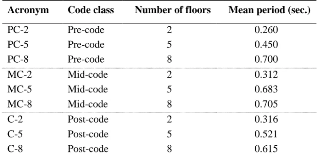
Table 2.1– Total area of exposed assets in 36 European capitals, and corresponding hazard level defined by the peak ground acceleration (PGA) with 10% exceedance probability in 50 years ... 24 Table 3.1– Considered building classes and corresponding fundamental periods of vibration ... 32 Table 3.2– List of rupture parameters in Akkar & Bommer (2010) and Chiou & Youngs (2008). Rrup is the closest distance to the rupture surface, Rx is the shortest horizontal

distance to a line defined by extending the fault trace to infinity in both directions, and Rjb is the Joyner-Boore distance. ... 35

(24)

(25)

Chapter 1 INTRODUCTION

1.1 Earthquake risk

Seismic action is paramount among natural hazards impacting civil infrastructure and human activity all over the globe (Ellingwood & Kinali, 2009). Major earthquakes have been responsible for a death toll of over 60,000 people per year in the last decades, as well as economic losses that can reach a great fraction of a country’s welfare (Silva, 2013). In Europe, countries such as Romania, Greece, Turkey and Italy, in particular, have experienced substantial material destruction and loss of life in the past 50 years, despite significant advances in building construction and design standards.

In the United States, the Northridge earthquake of 1994 is perhaps the most important in a series of events registered in California over the past 30 years. It will long be remembered for the unprecedented losses incurred as a result of a moderate-size event, which amount to as much as 40 billion USD, excluding indirect effects (Eguchi, et al., 1998). This makes the Northridge earthquake identically severe to the Kobe event that occurred exactly one year after, in Japan, adding to the reality that developed countries are equally exposed to high earthquake risks. In this context, the Great East Japan Earthquake and tsunami (2011) sent a clear message to countries and regions believed to be prepared to cope with seismic hazard. In fact, the year of 2011 was the most expensive year ever registered, far exceeding the 2005 economic losses, which held the previous record mainly due to the effects of hurricane Katrina. From the overall cost of 380 billion USD, the earthquake disasters in Japan and New Zealand alone accounted for 60% of this value (Silva, 2013).

(26)

2 Chapter 1

1.2 Earthquake loss modelling and uncertainties

Earthquake losses have a crippling effect on the economy of affected countries, either by the legal liability of governments to cover the full costs of rebuilding, and/or by the financial burden imposed upon private companies and individuals. In the face of this problem, earthquake loss modelling serves as the foundation to risk prediction and prevention, as a way to mitigate the adverse impacts of future events. A particularly relevant example is the creation of the Turkish Catastrophe Insurance Pool (TCIP), after the enormous financial burden imposed by the 1999 Kocaeli and Duzce earthquakes, due to the country’s statuary obligation in covering the costs of reconstruction. By means of this initiative, the creation of an earthquake loss model allowed a large part of the financial risk to be transferred to the world’s reinsurance markets, further enabling the evaluation of catastrophe risk impacts in the Turkish economy (Bommer, et al., 2002).

Earthquake loss modelling also serves as the base to many other seismic risk mitigation actions. These may include prioritization of zones within a country where the structural seismic vulnerability of the building stock should be improved, planning of post-disaster emergency response, or definition of mandatory seismic-proof construction practices (Silva, 2013). However, the required resources, datasets and tools seldom exist in a way that is compatible with a comprehensive assessment of seismic risk. Despite of great advances made in the last decades in the areas of: probabilistic seismic hazard assessment (e.g. Abrahamson (2006), Bommer & Abrahamson (2006)), evaluation of building vulnerability (e.g. Calvi et. al. (2006)), and collection of information regarding elements exposed to hazard (e.g. Dell’Acqua et. al. (2013)), several limitations still exist in the way that uncertainties in each of these aspects can consistently be taken into account. In the presence of uncertainties, risk to civil infrastructure from earthquakes cannot be eliminated, but must be managed in the public interest by the entities involved in its evaluation (Ellingwood & Kinali, 2009). Therefore, any meaningful seismic risk or safety assessment must be fully-coupled with its accompanying analysis of uncertainty, be that aleatory or knowledge-based (i.e. epistemic).

Structural reliability concepts and probabilistic risk analysis tools (e.g. Silva et. al. (2014)) provide an essential framework to model uncertainties associated with earthquake prediction, exposure definition, and infrastructure response. In addition to the continued improvement in the characterization of random and epistemic uncertainties in seismic hazard, recent years have seen a major swing in emphasis towards the explicit inclusion

(27)

Chapter 1 3

of uncertainties in the performance assessment of single buildings (Bradley, 2013). These have been mainly related with the treatment of sources of uncertainty such as the (hazard-consistent) record-to-record variability and/or the random nature of geometric and structural parameters (e.g. Jalayer et. al. (2010)), in the evaluation of the seismic response. However, in the context of portfolio risk assessment, several important questions remain entirely unanswered or lack a deepest understanding.

The main focus of this thesis consists of the treatment of random and epistemic uncertainties in the hazard-consistent evaluation of building fragility, vulnerability and risk assessments. Matters of statistical significance and spatial correlation of damage and loss are investigated in the context of the probabilistic loss estimation of building portfolios. As a result, innovative methodologies for the treatment of uncertainties are proposed, demonstrating its increased accuracy and robustness when compared with state-of-the-art risk assessment frameworks.

1.3 Objectives and thesis organization

With the aim of addressing several important issues related with the treatment of uncertainties in the earthquake loss modelling of building portfolios, the present thesis is divided into seven chapters. The first and present one consists of an introductory presentation of the various subjects addressed in this thesis, Chapter 7 discusses the main conclusions and possible future developments, and the remaining five chapters can further be grouped into two main subjects: building exposure and vulnerability. With regard to the former, Chapter 2 deals with current limitations in the development of exposure datasets of buildings of industrial use, at the European scale, whereas Chapter 3 to Chapter 6 are concerned with the treatment of random and epistemic uncertainty in the development of fragility and vulnerability models for loss estimation of building portfolios. More specifically, Chapter 3 presents the study of the impact of simplifications generally accepted as state-of-the-art by researchers and practitioners, in the context of seismic hazard disaggregation and record selection for fragility analysis and earthquake loss estimation, Chapter 4 consists of the evaluation of several sources of uncertainty in the process of analytically deriving fragility functions for the loss estimation of building portfolios, Chapter 5 addresses the modelling of spatial correlation of vulnerability uncertainty in portfolio risk analysis, and Chapter 6 deals with the study of the impact of epistemic uncertainty in the development of hazard-consistent fragility models and

(28)

4 Chapter 1

corresponding risk estimates. The contents of each chapter are subsequently described in further detail.

The second chapter presents the recent developments in Volunteered Geographic Information (VGI), such as the OpenStreetMap initiative, highlighting the potential of these datasets as supplementary or alternative sources of spatially-based building information. Its increase in usefulness is particularly evidenced when combined with additional Open-Access data such as the CORINE initiative, which provides the geo-referenced distribution of non-residential areas in Europe. In this context, this chapter presents the development of an algorithm that, based on open-access information, provides an automated tool for the development of exposure datasets of industrial buildings in Europe, at the 30 arc-second resolution.

The third chapter of this thesis sheds light on several problems and limitations in current practice of hazard-consistent ground-motion selection and fragility analysis, focusing on the impact that (commonly assumed) approximations in disaggregation outputs have on the distinct risk metrics, as opposed to an exact solution. These issues are investigated for several building typologies, seismicity models and ground motion prediction equations (GMPE), and appropriate guidelines are provided to researchers and practitioners.

In the fourth chapter, it is demonstrated that several questions exist regarding the appropriate treatment of structural capacity and seismic demand variability, from a statistical significance perspective, in the context of the fragility evaluation of building portfolios. As a result, matters such as: the minimum number of ground-motion records necessary for a statistically meaningful evaluation of structural response, the statistical significance of analytically determined damage exceedance probabilities, and the statistically meaningful representation of uncertainty and correlation in the estimation of intensity-dependent damage exceedance probabilities are addressed.

In the fifth chapter, the concepts developed in Chapter 4 are extended to the definition of building Vulnerability, whereby vulnerability functions are characterized by hazard-consistent distributions of damage ratio (i.e. ratio between cost to repair and total value of the building) per level of primary seismic intensity parameter. The latter is further included in a loss assessment framework, in which the impact of variability and spatial

(29)

Chapter 1 5

correlation of damage ratio in the probabilistic evaluation of seismic loss is accounted for, using several building portfolios as test-bed cases. The proposed methodology is evaluated in comparison with current state-of-the-art methods of vulnerability and loss calculation, highlighting the discrepancies that can arise in loss estimates when the variability and spatial distribution of damage ratio are not appropriately taken into account.

The sixth chapter consists of the application of the results and methodologies developed in Chapter 3, Chapter 4 and Chapter 5, with the aim of developing a statistically significant framework that allows the hazard-consistent propagation of uncertainty from fragility to loss estimates. In this study, several independent hazard modelling options are considered, in order to infer the repercussion from using fragility functions that are consistent with each hazard modelling approach, on the appraised risk metrics. In light of the appraised results, a methodology for the fragility assessment of building portfolios is presented, in which the epistemic uncertainty of the hazard model can be adequately propagated into the fragility results.

Finally, Chapter 7 summarizes the main conclusions of the present work, providing a description of future developments that, in light of the presented findings, are envisaged in order to improve the results and methodologies addressed herein.

(30)

6 Chapter 1 This page is intentionally left blank

(31)

Chapter 2 USING

OPEN-ACCESS

DATA

IN

THE

DEVELOPMENT

OF

EXPOSURE

DATASETS

OF

INDUSTRIAL BUILDINGS

This chapter is based on the following reference:

Sousa, L.; Silva, V.; Bazzurro, P (2017) Using open-access data in the development of exposure datasets of industrial buildings for earthquake risk modelling. Earthquake Spectra, 33(1): 63-84. doi: 10.1193/020316EQS027M

Summary

Recent developments in Volunteered Geographic Information (VGI), such as the OpenStreetMap (OSM) initiative, highlight the potential of these datasets as supplementary or alternative sources of spatially-based building information. Its increase in usefulness is particularly evident when combined with additional Open-Access data such as the CORINE initiative, which provides the geo-referenced distribution of non-residential areas in Europe. However, the systematic application of VGI in the development of exposure models for catastrophe risk assessment has been the subject of limited research. This chapter describes an algorithm that, based on open-access information, provides an automated tool for the development of exposure datasets of industrial buildings in Europe, at the 30 arc-second resolution. Its practical application shows that results obtained at national and regional scales are in excellent agreement with data collected from cadastral agencies in Denmark, Italy and Portugal, which highlights the potential of the algorithm when real building information is scarce or non-existent.

2.1 Introduction

Earthquake impacts in buildings of industrial use have been particularly relevant in recent events, highlighting the importance of a detailed modelling of direct and indirect losses resulting from this type of structures.

The widespread damage to welded steel moment resisting frame systems that happened in different types of buildings including industrial facilities, was one of the

(32)

8 Chapter 2

major overall lessons of the Northridge earthquake (Youssef, Bonowitz, & Gross, 1995) that occurred in 1994 in Southern California. In this event, damage occurred in new as well as old buildings, despite the fact that most damaged structures were constructed according to modern codes and standards of practice. In the case of the Kocaeli earthquake, which hit north-western Turkey in 1999, extensive damage to industrial buildings has been reported in a region where approximately forty percent of heavy industry in Turkey was concentrated (Sezen & Whittaker, 2004). The widespread damage to industrial facilities had a substantial impact on the economy of the region in terms of direct losses resulting from structural and non-structural damage, and from indirect losses stemming from business interruption, loss of utilities and loss of transportation infrastructure. The relevance of these findings is extremely important considering that many of the inspected structures were designed in accordance with U.S. and European standards, providing valuable indications as to the likely performance of industrial facilities in other seismically active regions of the world.

In Europe, evidence of satisfactory earthquake response goes hand in hand with reports of collapse of precast buildings, which is the most commonly structural typology used in industrial buildings (Bournas, Negro, & Taucer, 2014). In Italy, specifically, a seismic sequence struck the region of Emilia Romagna in 2012, with two main events on May 20th and May 29th, with local magnitude of 5.9 and 5.8, respectively. These earthquakes caused approximately three quarters of the precast concrete industrial buildings designed with non-seismic provisions in the affected area to suffer significant damage, with one quarter of the total presenting partial or total collapse of the roof. The severe damage that affected these buildings has been probably the most controversial issue raised by these events, given the high level of exposure in terms of human life, building contents, and the importance of the continuity of production processes in the socio-economic activity of the region.

In the context of risk assessment, characteristics such as occupancy type, geometry and material properties are essential to describe the uniqueness of each individual building or building class. However, the quantification of building stock, and the definition of its spatial distribution and structural characteristics are resource intensive and strenuous problems to tackle (Dell’Acqua, Gamba, & Jaiswal, 2013).

Due to the several practical challenges, the engineering and loss modelling community often rely on aggregated statistical data on building stock as the input to the loss estimation procedure. Of course, the various census datasets, collected by national

(33)

Chapter 2 9

statistical offices, are an important source of building inventory, providing rigorous and detailed information unlike any other dataset at a national scale. However, because statistical offices do not usually allow public users to access data at the building level, and independent field surveys are impractical for relatively large regions, the building datasets used for the purposes of exposure modelling are usually coarse in their spatial resolution.

Unfortunately, be it parish, municipality, regional or national level, the use of aggregated portfolios can introduce significant errors in risk assessment procedures due to the unbalanced spatial distribution of the building stock with respect to the considered hazard (Bazzurro & Park (2007) and Silva et. al. (2015b)). Thus, disaggregating an exposure dataset at a finer resolution but still compatible with available computational resources is of utmost importance. A suitable level of disaggregation is not self-evident and is also peril dependent. For example, losses estimated for natural events such as earthquakes are still sensitive to the level of detail of the location of the exposed assets (e.g., due to local site effects) but less so than events with narrower and more irregular footprints, such as hailstorms or floods (Chen, et al., 2004).

In the context of earthquake loss estimation, several sources of proxy data are routinely used in the regional disaggregation of coarse exposure datasets. Population density is arguably the more readily available and easy to apply, as demonstrated by Silva et. al. (2015b) in the disaggregation of the Portuguese building stock at parish level based on the population distribution on a 30 arc sec grid. This is a reasonable and well-established approach in the case of residential and public buildings, for which there is an obvious correlation between population density and built-up area. However, this approach is generally not robust for commercial and industrial buildings, which, because of their use, are usually located outside residential areas.

In the case of industrial buildings, not only census data or other type of cadastral information are extremely difficult to obtain at any level of regional aggregation, but also spatial disaggregation methods typically applied in residential building portfolios are not suitable. As a result, alternative approaches need to be explored, particularly with respect to sources of spatial-based building data. In this chapter, attention is given to open-access datasets and Volunteered Geographic Information, including the information provided by the CORINE and OpenStreetMap initiatives in an automated tool for the development of exposure datasets of industrial buildings.

(34)

10 Chapter 2

2.2 Objective and area of interest

In this study we describe a methodology that, based on open-access datasets and Volunteered Geographic Information, allows users to automatically develop geo-referenced exposure datasets of industrial buildings in the region of interest. Given the nature of the OSM information, which provides distinct degrees of completeness (Hecht, Kunze, & Hahmann, 2013) in different locations, particular focus is given to the development of methods that are able to identify and overcome possible data shortage, in a statistically meaningful way.

Following a detailed presentation of the datasets, the methodology proposed herein is validated by comparing exposure models derived for Denmark, Italy and Portugal (at different regional scales) with real data independently collected from mapping and cadastral agencies in those countries. In order to demonstrate the algorithm capabilities, exposure datasets are additionally derived for the 36 European countries: Albania, Austria, Belgium, Bosnia and Herzegovina, Bulgaria, Croatia, Cyprus, Czech Republic, Denmark, Estonia, Finland, France, Germany, Hungary, Iceland, Ireland, Italy, Latvia, Lithuania, Luxembourg, Malta, Macedonia, Montenegro, Netherlands, Norway, Poland, Portugal, Romania, Serbia, Slovakia, Slovenia, Spain, Sweden, Switzerland, Turkey and United Kingdom. Results are computed with a spatial resolution of 30 arc-seconds, and further aggregated at the first administrative level in each country, for visual clarity. These databases were utilized to underpin the earthquake loss estimation models developed for Europe by RED and ERN (www.redpavia.com).

2.3 Input data

2.3.1 CORINE

The IMAGE 2000 & CORINE Land Cover project (EEA-ETC/TE, 2002) was launched in 1994 by the European Environmental Agency (EAA) and the Joint Research Centre (JRC) of the European Commission. Its main objective was to provide an up-to-date land cover database, as well as information regarding general land cover changes in Europe between 1990 and 2000 (Steenmans & Perdigao, 2001).

These datasets were derived from satellite imagery and other ancillary data such as aerial photos, digital elevation datasets and hydrology models. As a result, CORINE classifies the European territory into 44 classes at a spatial detail comparable to that of a

(35)

Chapter 2 11

paper map on a scale of 1:100,000. Amongst the total set of identified land cover classes, the industrial and commercial units are of interest for this research, as further presented in detail. According to the CORINE technical guide (Bossard, Feranec, & Otahel, 2000), these units correspond to areas mainly occupied by industrial activities of transformation and manufacturing, trade, financial activities and services. For the sake of synthesis, these mixed activity areas are referred herein as non-residential areas, and their location is shown in Figure 2.1.

2.3.2 OpenStreetMap (OSM)

OpenStreetMap (OSM) is a collaborative project founded in 2004 in the University College London, with the aim of creating a free geographic database of the entire world (Ramm, Topf, & Chilton, 2010). Its launch marked a new approach to gathering geodata, made possible by the increasing proliferation of GPS devices amongst private users and by the availability of web-based mapping services. In the case of exposure datasets for earthquake loss assessment specifically for industrial buildings, several georeferenced features provided by OSM are of interest. Available information regarding building footprints and location, building height and land use areas are of evident and increasing usefulness, especially when combined with additional open-access sources such as the CORINE initiative (Bossard, Feranec, & Otahel, 2000).

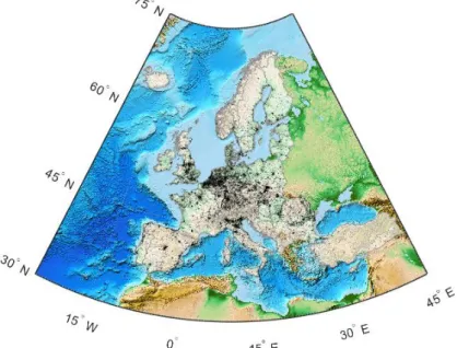
Figure 2.1 – Georeferenced database of non-residential areas (black) provided by the CORINE Land Cover project (CORINE, 2006) for 36 European countries.

Because many sources of geographic data, even those publicly available, are provided with restrictions to their use, OSM’s data are distributed under the “Creative

(36)

12 Chapter 2

Commons Attribute-ShareAlike 2.0 license”, which allows freedom of use by the public (Girres & Touya, 2010).

OSM is probably the most popular and successful VGI initiative, as supported by recent investigations on its completeness and quality. As demonstrated by Haklay (2010) and by Neis et al. (2012), urban areas in Central Europe have already been partially mapped with an impressive level of detail, and OSM is well ahead of only mapping the street network. A plethora of spatial data such as roads, buildings, land use areas or points of interest exist in the project’s database (OSM Statistics , 2015), emphasizing the potential of its use in the development of catastrophe exposure models in Europe. However, as further highlighted in this chapter, information regarding building height, type of material and age of construction is not provided in a large number of cases. Moreover, each building footprint might enclose several structures, which carries an important limitation when the actual number of assets is of interest.

In this study, data concerning building location and footprint, height, area and land use are used as input for the proposed algorithm, and issues related to the aforementioned data completeness are addressed in their systematic application.

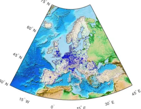
For the sake of illustration, Figure 2.2 presents the industrial land use areas provided by the OSM for the aforementioned 36 European countries, as of October 2015.

Figure 2.2 – Industrial land use areas provided by the OSM database (blue) for 36 European countries, as of October 2015.

(37)

Chapter 2 13

2.4 Methodology and algorithm

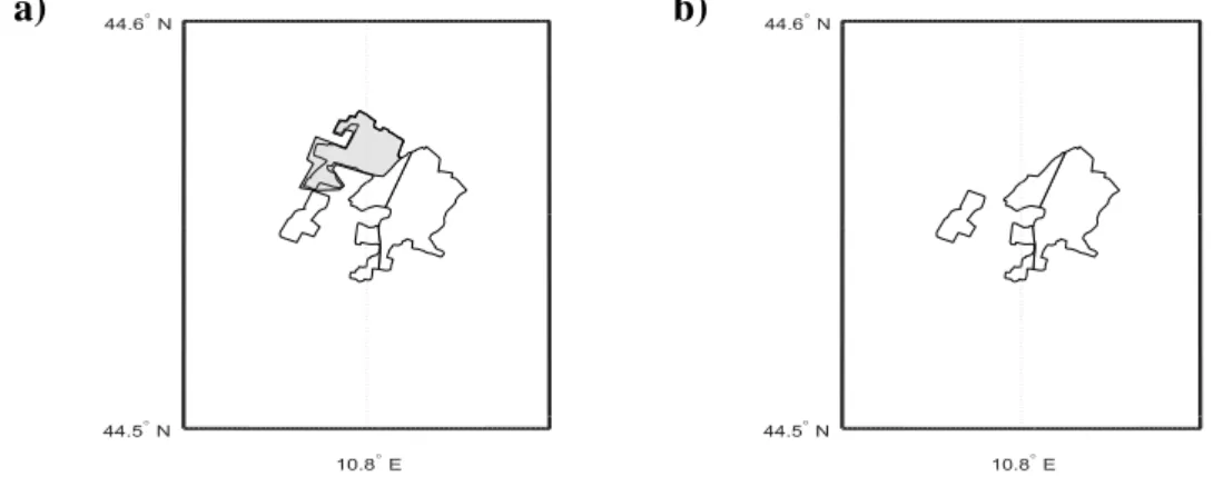
The general methodology and the corresponding algorithm developed in this research study are schematically presented in Figure 2.3. Starting from the envelope of non-residential areas containing undifferentiated industrial and commercial units (CORINE), the algorithm identifies areas containing only industrial (not commercial) assets via the Area Calculator. The identification is based on the input from OSM, which includes differentiated industrial and commercial areas (see Figure 2.4). Note that in this framework we use OSM information only when complete (i.e., whenever it accurately reflects the reality of the industrial built inventory). Issues concerning data completeness are addressed later in this study.

The various identified polygons containing industrial assets (Figure 2.4b) are further used to determine the footprints of all the industrial buildings inside, as provided by the OSM datasets (Figure 2.5). It shall be mentioned that, in some rare cases, a footprint may include more than one structure, a caveat that should be kept in mind in those rare applications when a precise building count is of interest. However, this is not relevant in the present situation, where only the total footprint area matters.

(38)

14 Chapter 2

The outcome of this process is the total industrial built area in a given region, obtained by inferring the number of floors of each building from the total height associated to the corresponding footprint (extracted from OSM). The final database is assembled by the Spatial Aggregation Calculator, in which the total area of all the industrial buildings determined as a function of building’s footprint and height are aggregated in a grid of 30 arc sec spacing, such as the one depicted in Figure 2.5b.

a) b)

Figure 2.4 – Schematic representation of the operations performed by the Area Calculator for an example area: a) Inputs: CORINE non-residential area (white) and OSM commercial area (grey),

and b) Industrial area output.

a) b)

Figure 2.5 – Schematic representation of the operations performed by the Building Exposure Calculator for an example area: a) Inputs, and b) Building-by-building output.

2.4.1 Data completeness

In order to overcome potential lack of data in a statistically robust way, particular attention is given to the level of completeness of the datasets. Assuming that a satisfactory level of coverage is provided by CORINE (i.e., all the non-residential areas in Europe are mapped), an “ideal” model would identify both building footprint and height of all the industrial buildings inside the CORINE polygons using OSM as input.

However, such a level of completeness cannot realistically be expected everywhere. At the time of this writing, some areas do have missing data as demonstrated by recent

(39)

Chapter 2 15

investigations by Haklay (2010) who reports the level of completeness of the OSM datasets in Europe. Thus, in “data-incomplete” regions for which information provided by OSM is not exhaustive, the “actual” industrial built area in each of the CORINE polygons is estimated using statistical techniques. This is done here according to the optimization algorithm described in Figure 2.6.

Based on the CORINE polygons in which OSM data is complete, reference probabilistic joint distributions 𝑓(𝑥, 𝑦) – are empirically derived for: x = building height, and y = ratio between surface of industrial building footprints and total area of the corresponding CORINE polygon. It is possible that the height, x, of the industrial buildings is statistically dependent on the density of the built area within a polygon, which is expressed by y. It is assumed, however, that x|y is independent on the area of the CORINE polygon. As a result, the reference 𝑓(𝑥, 𝑦) distribution is used to jointly sample the values of these random variables x and y in the CORINE polygons with incomplete OSM data. This process is shown in Figure 2.6.

Development of Innovative Methodologies for the Treatment of Uncertainties in the Earthquake Loss Estimation of Building Portfolios

F

E

U

P

DEVELOPMENT OF INNOVATIVE

METHODOLOGIES FOR THE TREATMENT

OF UNCERTAINTIES IN THE EARTHQUAKE

LOSS ESTIMATION OF BUILDING

PORTFOLIOS

Luis Miguel Costa Sousa

F

E

U

P

DEVELOPMENT OF INNOVATIVE

METHODOLOGIES FOR THE

TREATMENT OF UNCERTAINTIES

IN THE EARTHQUAKE LOSS

ESTIMATION OF BUILDING

PORTFOLIOS

A thesis submitted to the Faculty of Engineering of the

University of Porto in fulfilment of the requirements for

the degree of Doctor of Philosophy

Scientific coordination of Dr. Mário António Lage Alves Marques,

post-doctoral researcher at the Faculty of Engineering of the University of Porto;

with co-supervision of Professor Humberto Salazar Amorim Varum, full

professor at the Faculty of Engineering of the University of Porto, and Dr.

Vitor Emanuel Marta da Silva, post-doctoral researcher at the Department

of Civil Engineering of the University of Aveiro

Orientação científica do Doutor Mário António Lage Alves Marques,

investigador post-doc da Faculdade de Engenharia da Universidade do

Porto; e coorientação do Professor Doutor Humberto Salazar Amorim

Varum, professor catedrático da Faculdade de Engenharia da Universidade

do Porto, e Doutor Vitor Emanuel Marta da Silva, investigador post-doc do

Abstract

Resumo

Acknowledgements

Contents

List of Figures

List of Tables

Chapter 1

INTRODUCTION

1.1 Earthquake risk

1.2 Earthquake loss modelling and uncertainties

1.3 Objectives and thesis organization

Chapter 2

USING

OPEN-ACCESS

DATA

IN

THE

DEVELOPMENT

OF

EXPOSURE

DATASETS

OF

INDUSTRIAL BUILDINGS

Summary

2.1 Introduction

2.2 Objective and area of interest

2.3 Input data

2.3.1 CORINE

2.3.2 OpenStreetMap (OSM)

2.4 Methodology and algorithm

2.4.1 Data completeness