The impact of the telecommunications sector on economic growth

M

ASTER

MONETARY AND FINANCIAL ECONOMICS

M

ASTERS

F

INAL

W

ORK

D

ISSERTATION

T

HE

I

MPACT OF THE

T

ELECOMMUNICATIONS

S

ECTOR

ON

E

CONOMIC

G

ROWTH

R

UI

F

ILIPE

C

ARDOSO

P

EDRO

M

ASTER

MONETARY AND FINANCIAL ECONOMICS

M

ASTERS

F

INAL

W

ORK

D

ISSERTATION

T

HE

I

MPACT OF THE

T

ELECOMMUNICATIONS

S

ECTOR

ON

E

CONOMIC

G

ROWTH

R

UI

F

ILIPE

C

ARDOSO

P

EDRO

S

:

N

R

Abstract

The objective of this work is to study whether the evolution of the telecommunication sector has any significant impact in the economic growth of Portugal and other regions of the world.

The telecommunications sector is one of the sectors that gained a relevant role in economic development worldwide. The acknowledgement of this sector has increased since the 90’s, with the development of several technologies that contribute to the rising of the consumption of this type of good and the evolution of its dynamic and structure.

Countries equipped with the more advanced telecommunications systems have been rapidly moving into post-industrial, information-based economic growth.

In this work the methodology used is panel data, with an empirical analysis of both developed and developing economies in the past two decades.

Keywords: Telecommunication Sector, Economic Growth, Information Technology JEL Codes: O47, L96, O33

Resumo

O objetivo desta dissertação é estudar se a evolução do sector das telecomunicações tem qualquer impacto significativo no crescimento económico de Portugal e outras regiões do mundo.

O sector das telecomunicações é um dos sectores que ganharam um papel relevante no desenvolvimento económico mundial. O reconhecimento deste sector tem aumentado desde os anos 90, com o desenvolvimento de várias tecnologias que contribuem para a subida do consumo deste tipo de bem, a evolução da sua estrutura e dinâmica.

Países equipados com os sistemas de telecomunicações mais avançados conseguiram evoluir rapidamente para uma era pós-industrial, com o crescimento económico baseado na informação.

Neste trabalho, a metodologia utilizada é a de dados de painel, com uma análise empírica dos mercados desenvolvidos e em desenvolvimento nas últimas duas décadas.

Palavras-Chave: Setor das Telecomunicações, Crescimento Económico, Tecnologias da Informação

Acknowledgments

I am grateful to my supervisor, Professor Nicoletta Rosati, for her patience, motivation, knowledge and support to accomplish this work.

I am also very grateful to my family, specially my wife, my parents and my brother for their unconditional support and constant encouragement, essential to my academic and personal development. This is dedicated to them.

Contents

4. ESTIMATION METHODS AND RESULTS ... 21

4.1 THE RESULTS ... 22

5. CONCLUSIONS ... 27

6. REFERENCES ... 29

APPENDIX A – LITERATURE REVIEW SUMMARY ... 34

APPENDIX B – SAMPLE STATISTICS ... 35

List of Figures and Tables

Figure 1 - World Growth rate of GDP pc and Telecommunications from 1995-2014 .. 35

Figure 2 - World Telecommunications subscribers (per 100 people) from 1995-2014 . 35 Figure 3 - Average Telecommunications subs. (per 100 people) from 1995-2014 ... 35

Table I– Summary of the variables presented in the study... 19

Table II – Descriptive statistics for panel - 150 countries, time period: 2000-2014 ... 20

Table III - Literature review summary ... 34

Table IV – GDP per capita and Total of Telecommunications by state of development 36 Table V – List of Countries considered by Continent, Sub-Region and Income Group 40 Table VI - Correlation matrix for total samples, time period: 2000-2014 ... 42

Table VII – Summary of results of estimation of equation (5), where Tel t ... 43

Table VIII – Summary of results of estimation of equation (6), where Tel t-1... 44

1. Introduction

Over time, telecommunications have suffered a huge transformation. The only constant pattern that persists on this type of sector is change. Together with technology, the telecom industry has been expanding rapidly and, although more slowly in recent years partly due to the recent global financial crisis, it is still growing every year (as we can see in Figure 1 in Appendix B). Additionally, this expansion has also been provoked by a reduction of costs (Leff, 1984) and also increasing capacity (Nadiri and Nandi, 2003). The liberalization and introduction of competition in this type of market has also helped growth and the technological development.

Despite the fact that the growth of the telecommunications sector has started some years earlier in the high income economies, since the beginning of the millennium countries with less developed economies, categorized as lower middle income and low income, have shown the higher rates of growth. Nevertheless, we assist in all type of income groups and regions a continuous growth over the time (see Figure 2 and Figure 3 in Appendix B).

There are several ways in which telecommunications can contribute to economic and societal development, direct and indirectly, but we would like to emphasize at least four of them: first, business retention; second, economic diversification; third, enhancement of quality of life; and fourth increasing business competitiveness (Pradhan et al, 2014).

Another important input to this subject, also defended by many authors, is that “if the telephone does have an impact on a nation’s economy, it will be through the

improvement of the capabilities of managers to communicate with each other rapidly over increased distances” (Hardy, 1980, page 279).

Telecommunications have gained much interest in economic research, because of the existence of network externalities, that means it increases the value with the increase of the number of users (see, for instance Kim et al, 1997 and Roller & Waverman, 2001). Others authors developed their research by looking at the direction of causality, as defended by Jipp (1963), between telecommunications and economic growth (see Cronin et al, 1991 and Pradhan et al, 2014).

In this perspective, some of the questions that we intend to answer are: first, seek whether the telecommunications sector is relevant to promote economic growth; second, whether there any evident different patterns in growth in different geographic zones or income groups provoked by the telecommunications sector; and third, study whether the recent international financial crisis impacted the evolution of the telecommunications sector.

To pursue our objectives, we construct an econometric analysis of the relationship between economic growth and the telecommunications, with the use of a panel data approach for 150 countries described in table V of Appendix B, for the period of 2000 to 2014. However, some countries were excluded, due to the lack of data. Our data includes the following five groups by geographical area: Worldwide, Africa, Americas, Europe, Asia & Oceania. Furthermore, we perform analysis for the following groups of income level and state of development: High Income, Upper Middle Income, Lower Middle Income, Low Income, Developed and Developing (Less Developed). These sub-groups are based on the classification of the International Telecommunications Union (ITU)

which follows the classification of the United Nations for statistical purposes, namely the M49.

The main conclusions reached are the following: (1) the telecommunications sector play a significant and important role in economic growth; (2) the differences between regions are significant, with the middle income countries, especially the upper middle income countries, producing a higher impact on economic growth by the investment on telecommunications than other type of income groups, and the developed countries having a higher impact on economic growth than those in development; (3) results also show that the correlation between telecommunications and the economic growth is not simply due to reverse causality, since the lagged values of telecommunications are statistically significant, which supports the point that this relationship is not due to reverse causality.

The remainder of this dissertation is organized as follows. In Section 2, a revision of the telecommunications sector theories is presented, together with some references regarding economic growth. Section 3, describes the sample and methodology. The tests and results are described in Section 4, and Section 5 concludes.

2. Literature Review

Many different theoretical models have been proposed to study economic growth, so the literature on this subject is very large, principally over the last two decades.

This work focuses on one aspect in particular, that is the debate on whether the contribution of the telecommunications sector is one of the reasons that move economic growth, despite the recent financial crisis. Therefore, we will review in the following the most important findings on the relationship of Economic Growth with Telecommunications.

One of the first studies that confirm a clear positive correlation is the work of Jipp A. (1963). Using data for different countries, the author identified for the first time a positive link between the per capita GDP and the indicators of telephone density, also named as Jipp Curve, but this statistical correlation does not prove causality.

Years later, another also pioneering study was the work of Andrew P. Hardy (1980), which investigates the telephone's role as a contributory agent in economic development. Using statistical information for 60 countries over 13 years, and applying cross-lagged correlation techniques to the time series, he determines and confirms that the telephone can contribute to economic development.

After this contributions, many are the studies that have analyzed the relationship between economic growth and telecommunications sector, with several types of analysis, applications and different economic schools of thought. For example, Lichtenberg (1995), Greenstein and Spiller (1996) and Madden and Savage (1998), explain different causes and contributions of telecommunications sector on economic growth.

Lichtenberg F. (1995), for the period of 1988-91, studied the contributions of capital and labor deployed in information systems at a firm level. The main conclusions are that the estimation of the production function suggests the existence of a considerable excess returns to capital and labor in information systems, but with a larger size and significance of the excess returns to capital.

Greenstein, S. M. & Spiller, P. T. (1996), examine a more specific question, the investment by local exchange telephone companies in optical fiber cable (lines and signal software), defending that it plays an important role in local telephone networks by bringing digital technology. In their main conclusions, we can see a confirmation of consumer demand being sensitive to investment in technology, especially the optical fiber cable, and also that the growth in consumer surplus and the business local revenues are increased by the investment in this infrastructure.

Madden G. & Savage S. J. (2000), continue the same line of thinking and study the relationship between gross fixed investment, telecommunications infrastructure investment and economic growth for Central and Eastern Europe. Conclusions confirm evidence of growth preceding investment, indicating an accelerator type mechanism.

However, these approaches have some limitations as they did not include more complex and structural models and also neglected a bidirectional causality analysis of telecommunications and economic growth. On the one hand, some authors argued that the bidirectional causality between telecommunications and economics plays an important role. Although there already exist some inconclusive results on the direction of causality, in the seminal work of Cronin et al (1991) was discovered a two-way relationship between both variables in the United States, and more recently Pradhan et al (2014), raised again this possibility by confirming a difference between the short-run and

the long-run results. Cronin et al (1993a, 1993b), additionally indicated that investment in this infrastructure was a reliable predictor of national productivity.

On the other hand, using structural models helps analyzing better the correlation of the development of telecommunications sector and economic growth, since controlling for some macroeconomic variables they allow to isolate the direct effect of infrastructure on growth. Examples of applications of these models are for instance Dholakia and Harlam (1994), Roller and Waverman (2001), Datta and Agarwal, (2004) and Shiu and Lam, (2008, 2010), which will be discussed in the following.

In Dholakia R. R. and Harlam B. (1994), investment in the telecommunications infrastructure is justified because of the positive influence on economic development. Results of an econometric analysis of data from 50 states of the United States of America suggests a very strong influence when it is viewed as the only developmental input as well as when it is compared with other infrastructures. Findings also suggests that it is not a question of simple trade-offs between investment in one input with that of another. Instead, investment has to be made in multiple infrastructures.

In the contribution of Roller and Wavermen (2001), a model is estimated by nonlinear general methods of moments for a sample of 21 OECD countries over a 20-year period, and, to pick up economy wide effects, the micromodel is estimated with the macro production function. Results show that telecommunications infrastructure has a positive effect on economic growth, and also that increases in this type of infrastructure could create higher growth effects than in less-developed non-OECD countries.

Datta and Agarwal (2004) use a dynamic panel data method in order to investigate the long run relationship between telecommunications and economic growth, correcting

for omitted variables bias, in a single equation cross-section regression; the results show a significant and positive correlation, after controlling for a number of other factors. Later the works of Ding et al (2008) and Batuo (2015) follow the same methodology, analyzing China and Africa, respectively.

Shiu and Lam (2008) construct a dynamic panel data to study the effect of the telecommunications infrastructure on the regional economic growth across China. Results indicate a positive relationship between the two variables, and that causality is found only in the affluent provinces. Nevertheless, in the central and western provinces the improvement in telecommunications infrastructure by itself is not sufficient for stimulating growth. Years later, Shiu and Lam (2010), using data from 105 countries and also applying a dynamic panel data to investigate this relationship, indicate that there is a bidirectional relationship between gross domestic product and telecommunications for the European and High Income Countries.

The main conclusions of the vast empirical literature around this relationship is that “telecommunications infrastructure does itself lead to growth because its products – cable, switches, and so forth – lead to increases in the demand for the goods and services used in their production” and also “the economic returns to telecommunications infrastructure investment are much greater that the returns on just the telecommunication investment itself.” (Roller and Waverman, 2001, page 909).

More recently, the work of Chakraborty & Nandi (2011) confirm that the impact on economic growth is expected to be higher when the investment is in telecommunications infrastructure rather than in other types of infrastructure.

Nevertheless, few studies compare the relationship worldwide. Can we say that all regions are sensitive to this relationship? Can we confirm the same relationship for the income distribution in general? Many defend that the impact is higher in countries with competition and privatization of the telecommunications sector than in those without it, and also that countries in the upper-middle income group can contribute for a higher economic growth than others (Shiu and Lam, 2010).

In the present work, therefore, an empirical analysis on recent data from most countries worldwide is performed, expecting to shed some light on the current global picture.

(Table III, in Appendix A, presents a brief summary of the literature review, where the main objectives and conclusions achieved are presented)

3. Empirical Analysis

This chapter has the main goal to describe the choice of the economic model and the database construction. First, the various empirical models used in the cited literature are reported, and the choice of the variables determining growth is discussed together with their expected effect. After this discussion, the model chosen for this study is presented, with a detailed discussion and justification of the chosen regressors. Finally, the total available sample is described, together with a proposal of sub-samples for a specific analyses by region and income groups.

3.1 The model

Among the large amount of models that exists to study the relations between economic growth and telecommunications, the methodology used in this work follows the works of Batuo M. (2015), Ding et al (2008) and Datta and Agarwal (2004); using dynamic panel data following Islam (1995), these works take into account the correlation between previous and subsequent values of growth, analyzing the telecommunications impact on economic growth in Africa, China and OECD countries, respectively. All this studies follow the growth equation approach by Barro (1991) and Barro and Sala-i-Martin (1997), in which the determinants of growth are examined including the conditional convergence hypotheses.

Conditional convergence occurs when the partial correlation between the variable growth and the initial level is negative Barro (1992). The growth equation, as we can see in Ding and Haynes (2006) and Ding et al (2008), including the telecommunications penetration, in the static specification of the model has the following form:

Where: 𝑖 - Indexes countries; 𝐺𝑅𝑇𝐻_𝑖- Annual growth rate of real GDP per capita for i; 𝑋_𝑖,0- Other conditioning variables; 𝑇𝐸𝐿_𝑖,0- Telecommunications penetration for i;

Although there is an unrealistic hypothesis of identical aggregate production functions across countries, Islam (1995) uses a dynamic panel data model that allows for unobservable individual effects. So the dynamic approach of the model, including country effects, has the following specification:

𝐿𝑛(𝐺𝐷𝑃)_𝑖,𝑡 = 𝛼₀+ 𝛽₁𝐿𝑛(𝐺𝐷𝑃)_{𝑖,𝑡−1}+ ∑_𝑗=2𝑛 𝛽_𝑗𝑋_𝑖,𝑡+ 𝛽_𝑛𝑇𝐸𝐿_𝑖,𝑡+ µ_𝑖 + 𝜂_𝑡+ 𝑣_𝑖𝑡 (2) Where: 𝑖 - Indexes countries; 𝑡 - Indexes time; 𝜂𝑡 - The unobserved time-effects;

𝑣_𝑖𝑡- The transitory error term; µ_𝑖 - Independent term that capture the country fixed effects; Following this approach, Datta and Agarwal (2004) used a panel data similar to Islam (1995), which includes the lagged growth rate and a lagged GDP per capita: 𝐺𝑅𝑇𝐻_𝑖𝑡 = 𝛼₀+ 𝛾𝐺𝑅𝑇𝐻_{𝑖,𝑡−1}+ 𝛽₁𝐿𝑛(𝐺𝐷𝑃)_{𝑖,𝑡−1}+ ∑𝑛_𝑗=2𝛽_𝑗𝑋_𝑖,𝑡+ 𝛽_𝑛𝑇𝐸𝐿_𝑖,𝑡+ µ_𝑖 + 𝜂_𝑡+

+ 𝑣_𝑖𝑡 (3)

In the same study, the same growth equation is extended to include the effects of telecommunications penetration on growth:

𝐺𝑅𝑇𝐻𝑖𝑡 = 𝛼0+ 𝛽1𝐺𝑅𝑇𝐻𝑖,𝑡−1+ 𝛽2𝐿𝑛(𝐺𝐷𝑃)𝑖,𝑡−1+ 𝛽3𝑃𝑂𝑃𝑖,𝑡+ 𝛽4𝐺𝐶/𝑌𝑖,𝑡+ 𝛽5𝐼/𝑌𝑖,𝑡+

+ 𝛽₆𝑂𝑃𝐸𝑁_𝑖,𝑡+ 𝛽₇𝑇𝐸𝐿_𝑖,𝑡 + µ_𝑖+ 𝜂_𝑡+ 𝑣_𝑖𝑡 (4)

In our empirical study, we chose the equation below, whose specification is explained in the following:

𝐺𝑅𝑇𝐻_𝑖𝑡 = 𝛼₀+ 𝛽₁𝐺𝑅𝑇𝐻_{𝑖,𝑡−1}+ 𝛽₂𝐿𝑛(𝐺𝐷𝑃)_{𝑖,𝑡−1}+ 𝛽₃𝑃𝑂𝑃_𝑖,𝑡+ 𝛽₄𝐿𝑛(𝐺𝐶/𝑌)_𝑖,𝑡+ + 𝛽5𝐿𝑛(𝐼/𝑌)𝑖,𝑡+ 𝛽6𝐿𝑛(𝑂𝑃𝐸𝑁)𝑖,𝑡+ 𝛽7𝐿𝑛(𝑇𝐸𝐿)𝑖,𝑡+ µ𝑖+ 𝜂𝑡+ 𝑣𝑖𝑡 (5)

where the dependent variable is the rate of growth of real gross domestic product per

capita (GROWTHit), measured at current international prices.

The first independent variable is the one period lag of the rate of growth of real gross domestic product per capita (GROWTHi,t-1), where GDP is in the logarithmic scale.

The second variable is the logarithm of the one period lag of the real gross domestic product per capita (GDPi,t-1). The inclusion of this variable has the main goal to test the

convergence, so a negative sign is expected, in other words, to measure the effect of past levels of GDP on subsequent growth, a higher level of past GDP leads to lower subsequent growth.

Next we include the rate of growth of the population (POP), whose expected sign is negative, as a lower population growth relates to higher GDP per capita.

The fourth explanatory variable is the share of government consumption in GDP (𝐺𝑐_{/𝑌) as the ratio of government purchases to real GDP, and is measured in logarithm.}

The expected sign is negative as defended by Barro (1991), “government consumption lowers savings and growth through the distorting effects of taxation or government-expenditure programs”. Additionally, a fifth variable is included that measures the share of fixed investment in GDP (𝐼/𝑌), also in logarithm, and has a positive expected sign.

Next, we have the measure of the extent to which the country is integrated into the global economy (OPEN), which is calculated in logarithm and measured by the total of imports and exports in proportion of real gross domestic product. The expected sign is positive, according to the economic theory.

As seventh, we have the crucial variable of our study, the telecommunications penetration (TEL), which is measured as logarithm of the total of fixed telephone

subscriptions (per 100 people), fixed broadband subscriptions (per 100 people), mobile cellular subscriptions (per 100 people) and internet users (per 100 people). The application of the logarithm follows Batuo (2015), and is justified because of the exponential pattern of this variable over time. Other variables were also included to measure the total of the telecommunications penetration, namely the fixed broadband subscriptions (per 100 people), mobile cellular subscriptions (per 100 people) and internet users (per 100 people), justified by the fact of being well developed technologies1. The expected sign for telecommunication variable is positive.

The explanatory variables chosen, follows the works of Datta and Agarwal (2004) and Batuo (2015) and where chosen to perform a full comparative analysis to different regions and income groups, as mentioned in Section 3.2.. Also following this works, we we will also perform the estimation of a two other specifications, in order to confirm that the results are not simply due to reverse causality; variable TEL is therefore introduced in its lagged values at t-1 and t-2, giving rise to the following two alternative models: 𝐺𝑅𝑇𝐻_𝑖𝑡 = 𝛼₀+ 𝛽₁𝐺𝑅𝑇𝐻_{𝑖,𝑡−1}+ 𝛽₂𝐿𝑛(𝐺𝐷𝑃)_{𝑖,𝑡−1}+ 𝛽₃𝑃𝑂𝑃_𝑖,𝑡+ 𝛽₄𝐿𝑛(𝐺𝐶_/𝑌)

𝑖,𝑡+

+ 𝛽₅𝐿𝑛(𝐼/𝑌)_𝑖,𝑡+ 𝛽₆𝐿𝑛(𝑂𝑃𝐸𝑁)_𝑖,𝑡+ 𝛽₇𝐿𝑛(𝑇𝐸𝐿)_{𝑖,𝑡−1}+ µ_𝑖 + 𝜂_𝑡+ 𝑣_𝑖𝑡 (6) 𝐺𝑅𝑇𝐻_𝑖𝑡 = 𝛼₀+ 𝛽₁𝐺𝑅𝑇𝐻_{𝑖,𝑡−1}+ 𝛽₂𝐿𝑛(𝐺𝐷𝑃)_{𝑖,𝑡−1}+ 𝛽₃𝑃𝑂𝑃_𝑖,𝑡+ 𝛽₄𝐿𝑛(𝐺𝐶/𝑌)_𝑖,𝑡+ + 𝛽5𝐿𝑛(𝐼/𝑌)𝑖,𝑡+ 𝛽6𝐿𝑛(𝑂𝑃𝐸𝑁)𝑖,𝑡+ 𝛽7𝐿𝑛(𝑇𝐸𝐿)𝑖,𝑡−2+ µ𝑖 + 𝜂𝑡+ 𝑣𝑖𝑡 (7)

If the causal relationship is reversed, that is if growth influences telecommunication rather than vice-versa, then the lagged values of telecoms should not be significant. On the other hand, if the lagged telecom variables are significant, this confirms that telecommunications affect growth.

In summary, the control variables used, the unit of measure and expected signs of impact are described in Table I:

Table I– Summary of the variables presented in the study

Variable Name Unit of measure Exp. sign

Annual growth rate of the real GDP per

capita Growth Annual %

One year lag of growth rate of real GDP

per capita Growtht-1 Annual % Positive

Real GDP per capita measured in

purchasing power parity GDP Real Negative

Annual rate of growth of population POP Annual % Negative Share of government consumption in GDP 𝐺𝑐_{/𝑌 % of GDP Negative}

Share of fixed investment in GDP 𝐼/𝑌 % of GDP Positive Level of integration into global economy Open % of GDP Positive

Telecommunications penetration Tel Real Positive

Sources: Own elaboration, based on economic theory

3.2 The sample

As already mentioned, the objective of this empirical study is to test the existence of a positive link between the telecommunications sector and economic growth. To analyze this contribution, data were retrieved from the World Banks’s World Development (WDI) database, for the period 2000-2014, over 150 countries. Table II, presents a summary of indicators for the whole sample. Table IV of Appendix B presents detailed descriptive statistics for each country.

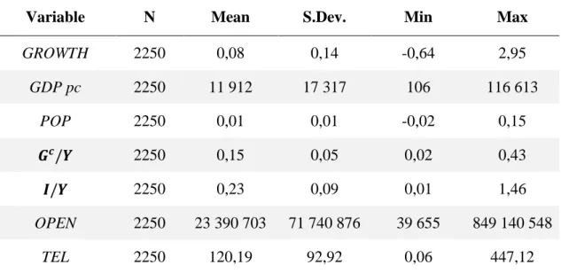
Table II – Descriptive statistics for panel - 150 countries, time period: 2000-2014

Variable N Mean S.Dev. Min Max

GROWTH 2250 0,08 0,14 -0,64 2,95 GDP pc 2250 11 912 17 317 106 116 613 POP 2250 0,01 0,01 -0,02 0,15 𝑮𝒄_{/𝒀 2250 0,15 0,05 0,02 0,43} 𝑰/𝒀 2250 0,23 0,09 0,01 1,46 OPEN 2250 23 390 703 71 740 876 39 655 849 140 548 TEL 2250 120,19 92,92 0,06 447,12

Sources: World Development Indicators – World Bank Note: N is the number of observations

This work will focus initially on the analysis of the total sample, and later on further subgroups divided by the following geographical areas: Africa (43); Americas (31), Europe (42) and Asia & Oceania (34). The inclusion of Oceania in Asia is justified for being a small sample to study. Furthermore, we will analyze the data for the following income groups and state of development, as rated by WDI and the ITU that follows the UN M49 database: High Income (49), Upper Middle Income (42), Lower Middle Income (35); Low Income (24); Developed (39); Developing (111). The countries included in each of the above groups are displayed in Table V of the Appendix B.

4. Estimation Methods and Results

To analyze whether the telecommunications influence economic growth, a panel data set is used, having cross-sectional and a time series dimension. There are several advantages of using panel data2_:

 Controlling unobserved heterogeneity – The techniques of panel data estimation can take such heterogeneity explicitly into account by allowing for individual-specific effects;

 Better suited to study the dynamics of change;

 Possibility to study more complex behavioral models;

In our analysis, we will consider the estimation of equations (5), (6) and (7), for the sub-groups mentioned before. The method of estimation employed is a GMM estimator, namely the difference GMM estimator, which was introduced by Holtz-Eakin, Newey, and Rosen (1990) and developed by Arellano and Bond (1991), designed for dynamic panel data models with few time periods and many individuals. Using linear GMM, the difference GMM executes the estimation after first-differencing the data, eliminating the fixed effects. This estimating procedure allows for the use of a set of internal instrumental variables, to deal with endogenous regressors, created from past observations of the instrumented variables (Roodman, 2008). Also, the robust estimation allows to deal with the presence of heteroskedasticity and serial correlation in the errors.

The most recent lags of the instrumented variables are indeed the best instruments, but they may be correlated with the error term, and this means that their validity can be

compromised. In order to test if that is the case, the Hansen test is performed, using the J statistic, where a high p value confirms the validity of the chosen instruments, and by consequence of the GMM results. However, in some cases the lags may turn out to be weak instruments for the first differenced model, especially if the autoregressive parameter is close to one. In these situations, an appropriate alternative is the system GMM estimator of Blundell and Bond (1998), where additional moment conditions are obtained from a level equation. A key condition to ensure that our estimation is consistent is that serial correlation of first order but not of second order should occur in the first difference model. These conditions can be tested using the Arellano-Bond test for autocorrelation. If a higher serial correlation is detected, than our instruments must be reviewed and redefined using older lags of the variables.

The software used for estimation is Stata 12.0 and the command performed is xtabond2 developed by Roodman (2006). The estimation is based on a two-step difference GMM estimator, with robust standard errors. Two-step difference GMM estimator is more efficient than one-step, providing the finite-sample correction to the covariance matrix proposed by Windmeijer (2005).

In summary, we perform a difference GMM in a two-step procedure with a robust estimation of the variance-covariance matrix, which means standard errors are robust to both heteroscedasticity and arbitrary patterns of autocorrelation within individuals.

4.1 The results

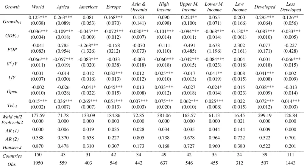
The estimation results for equation (5) are reported in Table VII in Appendix C, where we show the coefficient values, standard error in parentheses and significance reported at the 1%, 5% and 10% levels by ***, ** and *, respectively. Table VIII and

are not simply due to reverse causality. We perform the estimation of the model as described above, for the overall worldwide sample and for each of the proposed sub-group by region, income level and development stage, in order to make a complete comparative analysis.

The first overall picture of our results show confirmation of correct specification of the various aspects of the models: in the Arellano-Bond test for autocorrelation of the errors we reject the null hypothesis in AR (1), but we do not reject it in AR (2), as expected. Secondly, the Wald Test, which tests the global significance of the regression, is statistically significant. The Hansen J statistic, which is used to determine the validity of the over-identifying restrictions in the GMM model, confirms that our instruments are valid in all estimated models. The coefficients signs, when statistically significant, are according to our expectation as described before.

Starting to analyzing the first specification as in equation (5), we find that the past levels of Growth (𝐺𝑅𝑇𝐻𝑖,𝑡−1) are statistically significant in the total sample and almost

all sub-groups (with the exception of Americas, Asia & Oceania and Lower Middle Income). The sign is according to the economic theory, despite the recent financial crisis, which could be the reason for the lack of significance in some of the estimations.

Next, we have the past level of GDP per capita, which shows a negative coefficient, significant at 1% level in all the estimations. This supports the convergence hypothesis, that means that countries with higher levels of GDP per capita have a tendency to grow at a slower rate and that countries with a lower levels of GDP per capita grow faster. The share of government consumption in GDP which is measured by the variable 𝐺𝑐/𝑌 is negatively and significantly associated with economic growth, result that is in line with Barro (1990:121), where it is argued that government consumption diminishes savings

and the economic growth through the distorting effects of taxation or government-expenditure programs.

The population growth (POP), the share of fixed investment in GDP (𝐼/𝑌) and the level of integration into global economy (OPEN) are not statistically significant in the total sample, although they are significant in some sub-groups with smaller samples. For example, the population growth is only significant, with a negative impact, in America and Asia & Oceania, which could indicate that in general it is not a very relevant determinant of economic growth. The share of fixed investment in GDP has a positive and significant impact in Europe, Lower Middle Income and Developed countries. Finally, the level of integration into global economy is positive and statistically significant in Europe, High Income and Developed Countries, fact that in the case of Europe could be linked with the European Union being highly open. Nevertheless, an unexpected negative sign appears in America, Upper and Lower Middle Income, but it is only significant at a 10% level, and becomes non-significant in the models where we consider further lags of the telecom variable.

Finally, we verify that the Telecommunications Penetration is statistically significant at 1% level to explain economic growth in all groups and sub-groups of panels. In fact, this proves that there is a strong impact of telecommunications penetration on economic growth. The estimated coefficient indicates, for the total sample, that for an increase of 10 subscriptions (per 100 people) the growth rate of GDP per capita will increase by 0,18%. However, when we analyze the sub-groups findings, some differences are found between regions, income groups and stage of development. For regions, Europe shows a larger size of the influence of telecoms on economic growth than other regions,

results show that countries with Upper Middle Income can more easily influence economic growth by investing in this type of good, compared to countries in other income groups. By the level of development, results show that in Developed countries telecoms have a much higher impact on economic growth than in those in Development, and this could be due to technology changes being more easily accessed by the developed countries. Therefore, we can globally affirm that the telecommunications has a positive influence to the economic growth.

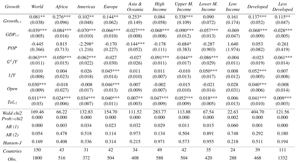
However, as already mentioned, in order to confirm that this relationship between telecommunications and economic growth is not due to reverse causality, we use the lagged values of the telecommunications and estimate equations (6) and (7), with the summary of the results showed in Table VIII and Table IX of Appendix C. Results show that telecommunications penetration does still have a positive impact even in its lags. This is confirmed by the coefficient of the one-lagged and the two-lagged values of the telecommunications penetration being positive and significant at the 1% level, although with a smaller magnitude when compared to the current value, with this result also being in line with the works of Datta and Agarwal (2004) and Batuo (2015). The only exceptions is the estimation of the effect for Low Income countries, where telecommunications are not statistically significant if lagged.

In summary, by the AR and Hansen tests results we have confirmation that our instruments are valid, and there is no evidence of serial correlation of second order in our first-difference estimation. Moreover, as expected, the results clearly confirm that telecommunications have a positive and solidly significant relationship with growth. Overall, the results are according to the initial expectations and do not underpin the economic theory. Finally, we verify that some variables are statistically significant to

explain economic growth only in some sub-groups of our sample of countries, and maybe this could depend on issues such as aging population, the ability of capital accumulation, and markets obstacles.

5. Conclusions

In this work, we explore the empirical relationship between telecommunications and economic growth with a sample of 150 countries, classified according to different regions of the world, different income levels and different state of development, over the period 2000 to 2014, and following the works of Batuo M. (2015), Ding et al (2008) and Datta and Agarwal (2004), using a dynamic panel data model.

The method of estimation employed is a difference GMM estimator, introduced by Holtz-Eakin, Newey, and Rosen (1990) and developed by Arellano and Bond (1991).

The telecommunications is both statistically significant and positively correlated to the GDP per capita growth for the overall worldwide model. When we analyze specific sub-groups of regions of countries, we see that Europe is the region where telecoms contribute more to the economic growth; likewise, in the analysis by income group, the upper middle income countries are those where the effect on economic growth is larger. This conclusion is consistent with the findings in Lam and Shiu (2010). For what concerns the countries’ level of development, results show that developed countries have a higher estimated impact than those in development, and such result could be explained by the constant technological changes being more easily accessed by the developed countries than those in development, and also due to the rapid spreading of information and a reduction of costs. The results also show, with the exception of Low Income countries, that the correlation between telecommunications and the economic growth is not simply due to reverse causality, since the lagged values of the telecommunications variable are statistically significant. The lagged GDP per capita has a negative and significant estimated effect on growth in all the samples, which supports the convergence hypothesis,

that means countries with higher levels of GDP per capita have a tendency to grow at a slower rate.

However, in the contribution that we made in the present work to the discussion on the interactions between the telecommunications and growth, there are some limitations in the analysis that we would like to point out: (1) we analyze the telecommunications penetration as a whole, and we could also seek, inside this infrastructure, which type of consumption good is more relevant to the economic growth by testing them separated as individual or grouped, for example groups of voice and internet; (2) some variables are not statistically significant in most of the models estimated in the sub-groups, and other variables were not available, such as those used in Ding et al. (2008), for example the share of total employment to total population and the human capital among others.

For further studies, we can also seek to investigate how the evolution of the telecommunications sector changes the composition of revenues of the market. The competition in local services where not analyzed and could explain some of the divergences between the sub-groups of estimation, namely whether the market structure is a monopoly, duopoly or in full competition. Last but not least, we could analyze if the difference on findings are due to the insufficiency of some countries’ infrastructure, and if less developed countries are behind other due to this insufficiency.

6. References

Arellano, M. & Bond, S. (1991). Some tests of specification for panel data: Monte Carlo evidence and an application to employment equations, Review of Economic Studies, 58, pp. 87-97.

Baltagi, B. (2005). Econometric Analysis of Panel Data. 3rd ed. s.1.:John Wiley. Barro, R. J. (1990). Government spending in a simple model of endogenous growth, Journal of Political Economy, 98, 5, pp. 407-443.

Barro, R. J. (1991). Economic Growth in a Cross Section of Countries, Quarterly Journal of Economics, Volume 106, No.2, pp. 407-443.

Barro R.J. & Sala-i-Martin, X. (1992). Convergence. Journal of Political Economy 100 (2), pp. 223 – 251.

Barro R.J. & Sala-i-Martin, X. (1997). Technological Diffusion, Convergence, and Growth. Journal of Economic Growth, 2: 1–27

Batuo, M (2015). The role of telecommunications infrastructure in the regional economic growth of Africa. The Journal of Developing Areas, Vol. 49 No. 1

Blundell, R. & Bond, S. (1998). Initial Conditions and Moment Restrictions in Dynamic Panel Data Models, Journal of Econometrics, Vol 87, 115-143.

Chakraborty, C., & Nandi, B. (2011). Main line telecommunications infrastructure, levels of development and economic growth: Evidence from a panel of developing countries. Telecommunications Policy, 35 (1), 441–449.

Cronin, F. J., Parker, E. B., Colleran, E. K., & Gold, M.A. (1991). Telecommunications infrastructure and economic growth: An analysis of causality. Telecommunications Policy, 15 (6), 529–535.

Cronin, F. J., Colleran, E. K., Herbert, P. L., & Lewitzky, S. (1993a). Telecommunications infrastructure investment and economic development. Telecommunications Policy, 17 (6), 415–430.

Cronin, F. J., Colleran, E. K., Herbert, P. L., & Lewitzky, S. (1993b). Telecommunications and growth: The contribution of telecommunications infrastructure investment to aggregate and sectoral productivity. Telecommunications Policy, 17 (9), 677–690.

Datta, A. & S. Agarwal. (2004). Telecommunications and Economic Growth: A Panel Data Approach. Applied Economics, Vol.36, No.15, 1649-1654.

Dholakia R. R. & Harlam B. (1994). Telecommunications and economic development: Econometric analysis of the US experience. Telecommunications policy, 18, 470-477

Ding, L. & Haynes, K. E. (2006). The role of telecommunications infrastructure in regional economic growth in china, Australasian Journal of Regional Studies, Vol. 12, No. 3, 281-302

Ding, L., Haynes, K. E. & Liu, Y. (2008). Telecommunications infrastructure and regional income convergence in China: panel data approaches, The Annals of Regional Science, Vol. 42, No. 4, pp 843–861

Greenstein, Shane and Spiller, Pablo T. (1996). Estimating the Welfare Effects of Digital Infrastructure. Working Paper No. 5770 National Bureau of Economic Research, Cambridge, MA.

Hardy, A. (1980). The role of telephone in economic development. Telecommunications Policy, Vol. 4(4), pp. 278–286

Holtz-Eakin, D., Newey, W., and Rosen, H. S. (1988). Estimating Vector Autoregressions with Panel Data. Econometrica Vol. 56, pp. 1371-1395.

International Telecommunication Union (2016). ITU Regions – ITU’s Telecommunication Development Bureau. [online] Available on: http://www.itu.int/en/ITU-D/Statistics/Pages/definitions/regions.aspx [Accessed 1 August 2016]

Islam, N. (1995). Growth empirics: a panel data approach. Quarterly Journal of Economics, Vol. 110, pp. 1127-1170

Jacobsen, K.F.L., (2003). Telecommunications – a means to economic growth in developing countries? In Development Studies and Human Rights. Chr. Michelsen Institute, Bergen.

Jipp A., (1963). Wealth of nation and telephone density. Telecommunications Journal, 30, 199-201.

Kim, D.H., Jae-Ho Juhn & Won-Gyu Ha, (1997). Dynamic Modeling of Competitive On-line Services in Korea. System Dynamics: An International Journal of Policy Modeling, Vol 9, nr. 2 : 1-23

Koutroumpis, P., (2009). The Economic Impact of Broadband on Growth: A simultaneous approach, Telecommunications Policy, 33, pp 471 – 485.

Leff, N. H., (1984). Externalities, information costs, and social benefit-cost analysis for economic development: an example from telecommunications. Economic Development and Cultural Change, 32(2), 255–76.

Lichtenberg F., (1995). The output contributions of computer equipment and personnel: a firm-level analysis. Economics of Innovation and New Technology 3, 201– 217.

Madden, G. & Savage, S.J., (1998). CEE telecommunications investment and economic growth. Information Economics and Policy, 10(2), 173–195.

Madden, G., & Savage, S. J., (2000). Telecommunications and economic growth. International Journal of Social Economics, 27 (7–10), 893–906.

Mileva, E, (2007). Using Arellano – Bond Dynamic Panel GMM Estimators in Stata - Tutorial with Examples using Stata 9.0. Economics Department, Fordham University, USA.

Nadiri, M. I. and Nandi, B., (2003). Telecommunication infrastructure and economic development. Working Paper

Pradhan, R., Arvin, M., Norman, N. and Bele, S., (2014). Economic growth and the development of telecommunications infrastructure in the G-20 countries: A panel-VAR approach. Telecommunications Policy, 38, 634–649.

Roodman, D., (2006). How to Do xtabond2: An Introduction to “Difference” and “System” GMM in Stata. Center of Global Development., No. 103

Roodman, D., (2008). A Note on the Theme of Too Many Instruments. Center of Global Development., No. 125

Roller, Lars-Hendrik, and Leonard Waverman., (2001). Telecommunications Infrastructure and Economic Development: A Simultaneous Approach., American Economic Review, 91(4): 909-923.

Shiu, A., & Lam, P., (2008). Causal relationship between telecommunications and economic growth in China and its regions. Regional Studies, 42 (5), 705–718.

Shiu, A., & Lam, P., (2010). Economic growth, telecommunications development and productivity growth of the telecommunications sector: Evidence around the world. Telecommunications Policy, 34 (4), 185–199.

United Nations (2016). Composition of macro geographical (continental) regions, geographical sub-regions, and selected economic and other groupings – United Nations

Statistics Division [online] Available at:

http://unstats.un.org/unsd/methods/m49/m49regin.htm [Accessed 1 August 2016] Wellenius, B., (1977). Telecommunications in developing countries, Telecommunications Policy, Vol. 1 (4), pp. 289–297.

Windmeijer, F., (2005). A finite sample correction for the variation of linear efficient twostep GMM estimators, Journal of Econometrics, 126, pp. 25-51.

World Bank (2016). World Development Indicators. Washington, DC: World Bank.

Appendix A – Literature review summary

Table III - Literature review summary

LITERATURE MAIN CONCLUSIONS

Hardy (1980) _{Telephones per capita had a significant impact on GDP, while the spread of radios did not.} Cronin et al (1991) _{Relationship between telecommunications and economic growth is a result of reverse causality} Dholakia & Harlam (1994) _{Positive relationship and that is not a question of simple trade-offs between investment in one input.}

Lichtenberg (1995) _{Considerable excess returns to capital and labor information systems}

Greenstein & Spiller (1996) _{Telecommunications infrastructure has a positive and significant effect on employment growth in the USA} Madden & Savage (1998) Positive contribution to development of economies and evidence of a bi-directional relationship Roller & Waverman (2001) Positive effect of telecommunications infrastructure on economic growth

Datta & Agarwal (2004) The results show a significant and positive correlation between telecommunications infrastructure and growth Ding et al (2008) System GMM estimation is more likely to produce consistent and efficient estimates than OLS and fixed-effect

estimation. Positive relationship between telecommunications and regional economic growth

Shiu and Lam (2008) There is a unidirectional relationship running from real GDP to telecommunications at the national level and improvement in telecommunications infrastructure alone is not sufficient for stimulating growth in all regions. Shiu & Lam (2010) Bidirectional relationship between real GDP and telecommunications. However, when the impact is measured

separately, the relationship is no longer restricted.

Pradhan,et al (2014) Find a bidirectional causality between development of telecommunications infrastructure and growth. Investment in telecommunications is subject to increasing returns, demonstrating that an increase in

Appendix B – Sample Statistics

Figure 1 - World Growth rate of GDP pc and Telecommunications from 1995-2014

Figure 2 - World Telecommunications subscribers (per 100 people) from 1995-2014

Figure 3 - Average Telecommunications subs. (per 100 people) from 1995-2014

0 50 100 150 200 250 300

High income Upper middle income Lower middle income Low income

Africa Américas Asia e Oceania Europa

​Developed ​Developing -10% -5% 0% 5% 10% 15% 20% 25% 30%

GDPpc Growth Teledensity Growth

0 20 40 60 80 100

Table IV – GDP per capita and Total of Telecommunications by state of development

State

DEVT Country

GDP per capita CAGR % Telecomunic. Subscribers CAGR % 2000 2014 00-14 2000 2014 00-14 -De ve loped Count rie s (3 9) Albania 1 176 4 589 10,2 5,64 179,54 28 Australia 21 665 61 996 7,8 143,39 282,34 5 Austria 24 517 51 148 5,4 162,21 298,75 4,5 Belarus 1 273 8 025 14,1 29,93 258,86 16,7 Belgium 23 207 47 300 5,2 134,7 275,93 5,3 Bulgaria 1 609 7 851 12 50,62 239,2 11,7 Canada 24 124 50 185 5,4 152,21 249,71 3,6 Czech Republic 5 995 19 502 8,8 89,97 255,77 7,7 Denmark 30 744 61 331 5,1 175,28 296,44 3,8 Estonia 4 070 20 148 12,1 107,62 305,55 7,7 Finland 24 253 49 865 5,3 164,99 276,08 3,7 France 22 466 42 547 4,7 121,1 285,17 6,3 Germany 23 719 47 767 5,1 148,39 299,28 5,1 Greece 12 043 21 627 4,3 114,64 248,74 5,7 Hungary 4 620 14 022 8,3 74,27 251,85 9,1 Iceland 31 737 52 037 3,6 191,54 296,65 3,2 Ireland 26 236 54 321 5,3 130,71 254,91 4,9 Italy 20 051 35 180 4,1 145,1 273,49 4,6 Japan 37 300 36 153 -0,2 133,08 290,21 5,7 Latvia 3 351 15 692 11,7 54,23 236,97 11,1 Lithuania 3 297 16 490 12,2 55,35 265,29 11,8 Luxembourg 48 992 116 613 6,4 149,5 329,47 5,8 Macedonia 1 875 5 453 7,9 32,85 208,55 14,1 Moldova 354 2 245 14,1 18,88 204,5 18,6 Netherlands 25 921 52 139 5,1 175,79 291,71 3,7 New Zealand 13 641 44 380 8,8 134,93 269,18 5,1 Norway 38 147 97 430 6,9 177,75 272,49 3,1 Poland 4 493 14 337 8,6 53,42 247,03 11,6 Portugal 11 502 22 124 4,8 123,27 245,62 5 Romania 1 668 10 012 13,7 32,19 199,59 13,9 Russian Fed. 1 772 13 902 15,9 26,05 270 18,2 Slovak Rep. 5 403 18 501 9,2 64,02 235,6 9,8 Slovenia 10 228 24 002 6,3 115,69 247,31 5,6 Spain 14 788 29 719 5,1 116,51 251,86 5,7 Sweden 29 283 58 900 5,1 188,57 293,66 3,2 Switzerland 37 813 85 611 6 185,69 319,78 4 Ukraine 636 3 065 11,9 23,62 221,42 17,3

State

DEVT Country

GDP per capita CAGR % Telecomunic. Subscribers CAGR % 2000 2014 00-14 2000 2014 00-14 DC Unit. Kingdom 26 401 46 279 4,1 160,38 304,92 4,7 United States 36 450 54 398 2,9 151,68 268,46 4,2 De ve lopi ng C ountrie s (1 11) Algeria 1 757 5 484 8,5 6,32 122,81 23,6 Angola 606 5 233 16,6 0,76 86,42 40,3

Antigua & Bar. 10 095 13 432 2,1 84,14 229,79 7,4 Argentina 7 669 12 751 3,7 46,01 262,04 13,2 Armenia 621 3 874 14 19,21 190,56 17,8 Azerbaijan 655 7 886 19,4 15,2 210,72 20,7 Bahamas, The 21 241 22 217 0,3 56,99 212,23 9,8 Bahrain 13 591 24 855 4,4 62,53 306,85 12 Bangladesh 407 1 087 7,3 0,65 92,2 42,4 Barbados 11 568 15 366 2 60,97 285,5 11,7 Belize 3 364 4 884 2,7 28 99,01 9,4 Benin 370 903 6,6 1,77 107,2 34,1 Bhutan 778 2 561 8,9 2,91 122,81 30,7 Bolivia 1 007 3 124 8,4 14,31 145,03 18 Botswana 3 333 7 153 5,6 23,3 195,73 16,4 Brazil 3 729 11 729 8,5 33,94 230,07 14,6 Brunei Dar. 18 155 40 980 6 61,89 197,38 8,6 Burkina Faso 227 713 8,5 0,75 81,88 39,8 Burundi 129 286 5,9 0,62 32,06 32,5 Cambodia 300 1 095 9,7 1,37 144,51 39,5 Cameroon 583 1 407 6,5 1,5 91,36 34,1 Central Afr. R. 245 352 2,6 0,45 28,59 34,5 Chad 166 1 025 13,9 0,23 42,51 45,4 Chile 5 229 14 566 7,6 60,03 238,86 10,4 China 955 7 587 16 19,75 173,85 16,8 Colombia 2 472 7 918 8,7 25,91 190,6 15,3 Comoros 372 810 5,7 1,55 61,21 30 Congo, D. Rep. 397 438 0,7 0,06 56,49 63,3 Congo, Rep. 1 036 3 147 8,3 2,97 115,63 29,9 Costa Rica 4 062 10 415 7 34,06 221,61 14,3 Cote d'Ivoire 649 1 546 6,4 4,8 122,62 26 Cyprus 14 307 27 246 4,7 85,06 215,23 6,9 Dominica 4 820 7 252 3 43,23 230,4 12,7 Dominican R. 2 802 6 147 5,8 22,17 145,79 14,4 Ecuador 1 451 6 346 11,1 15,08 170,43 18,9 Egypt, Arab R. 1 461 3 366 6,1 10,99 157,26 20,9 El Salvador 2 260 4 102 4,4 24,15 193,65 16

State

DEVT Country

GDP per capita CAGR % Telecomunic. Subscribers CAGR % 2000 2014 00-14 2000 2014 00-14 De ve lopi ng C ountrie s (1 11) Eq. Guinea 1 970 18 918 17,5 2,27 87,69 29,8 Gabon 4 115 10 772 7,1 14,19 182,9 20 Gambia, The 637 441 -2,6 4,09 138,26 28,6 Georgia 692 4 430 14,2 15,32 211,37 20,6 Ghana 265 1 442 12,9 1,97 134,97 35,2 Grenada 5 118 8 574 3,8 39,15 191,53 12 Guatemala 1 650 3 667 5,9 14,4 143,6 17,9 Guinea 340 540 3,3 0,85 73,83 37,5 Guinea-Bissau 281 616 5,8 1,1 67,17 34,1 Guyana 960 4 028 10,8 21,15 133,39 14,1 Honduras 1 138 2 434 5,6 8,48 120,37 20,9 H. Kong SAR 25 757 40 216 3,2 171,46 400,46 6,2 India 452 1 577 9,3 3,98 95,86 25,5 Indonesia 780 3 500 11,3 5,87 157,49 26,5 Iran, Islamic R. 1 664 5 443 8,8 16,79 175,67 18,3 Israel 21 052 37 206 4,2 143,49 257,22 4,3 Jordan 1 774 4 831 7,4 23,79 201,49 16,5 Kazakhstan 1 229 13 155 18,5 14,61 266,23 23 Kenya 409 1 368 9 1,66 117,82 35,6 Korea, Rep. 11 948 27 989 6,3 167,69 298,36 4,2 Kyrgyz Rep. 280 1 280 11,5 8,81 174,8 23,8 Lao PDR 324 1 751 12,8 1,1 94,77 37,4 Lebanon 5 335 8 149 3,1 48,72 205,29 10,8 Lesotho 416 1 034 6,7 2,57 98,05 29,7 Liberia 183 458 6,8 0,3 79,13 48,9 Macao SAR 14 128 96 075 14,7 88,07 447,12 12,3 Madagascar 246 467 4,7 0,95 46,07 32 Malawi 156 362 6,2 0,97 39,73 30,4 Malaysia 4 005 11 307 7,7 63,01 241,08 10,1 Mali 267 842 8,5 0,63 157,07 48,4 Mauritania 477 1 371 7,8 1,46 106,39 35,9 Mauritius 3 861 10 003 7 46,17 218,06 11,7 Mexico 6 650 10 351 3,2 30,52 154,86 12,3 Mongolia 474 4 202 16,9 12,61 146,83 19,2 Morocco 1 328 3 190 6,5 13,81 198,91 21 Mozambique 275 623 6 0,86 76,16 37,8 Namibia 2 059 5 343 7 11,77 138,13 19,2 Nepal 231 702 8,2 1,4 101,17 35,8

State

DEVT Country

GDP per capita CAGR % Telecomunic. Subscribers CAGR % 2000 2014 00-14 2000 2014 00-14 De ve lopi ng C ountrie s (1 11) Nigeria 378 3 203 16,5 0,54 120,63 47,2 Oman 8 711 19 310 5,9 21,03 242,04 19,1 Pakistan 535 1 315 6,6 2,34 90,86 29,9 Panama 4 062 12 712 8,5 34,04 225,86 14,5 Paraguay 1 546 4 713 8,3 21,38 156,41 15,3 Peru 1 967 6 549 9 14,58 159,41 18,6 Philippines 1 040 2 873 7,5 14,24 177,22 19,7 Rwanda 216 698 8,7 0,74 75,06 39,1 Saudi Arabia 8 809 24 406 7,6 23,76 278,97 19,2 Senegal 475 1 067 6 5,03 119,4 25,4 Sierra Leone 157 793 12,3 0,87 79,02 38,1 Singapore 23 793 56 007 6,3 157,55 291,79 4,5 South Africa 3 099 6 472 5,4 35,01 208,27 13,6 Sri Lanka 875 3 853 11,2 7 144,1 24,1 St. Kitts and N. 9 224 15 739 3,9 56,6 245 11 St. Lucia 4 975 7 648 3,1 37,84 186,87 12,1 St. Vincent 3 673 6 673 4,4 28,52 198,42 14,9 Sudan 353 1 876 12,7 1,22 97,97 36,8 Suriname 1 856 9 680 12,5 27,44 234,79 16,6 Tajikistan 139 1 113 16 3,6 117,93 28,3 Tanzania 308 955 8,4 0,95 68,1 35,7 Thailand 2 016 5 970 8,1 17,56 196,26 18,8 Togo 266 630 6,4 2,71 71,22 26,3 Tonga 1 927 4 114 5,6 12,52 117,33 17,3 Tri. & Tobago 6 431 21 317 8,9 45,47 251,48 13

Tunisia 2 248 4 329 4,8 14 187,67 20,4 Turkey 4 215 10 304 6,6 58,42 174,05 8,1 Uganda 261 715 7,5 0,94 71,27 36,2 U. A. Emirates 34 208 43 963 1,8 104,59 302,28 7,9 Uruguay 6 872 16 738 6,6 50,89 278,51 12,9 Uzbekistan 558 2 053 9,7 7,36 132,39 22,9 Vanuatu 1 470 3 148 5,6 5,89 83,2 20,8 Venezuela, RB 4 785 12 518 7,1 36,09 189,04 12,6 Vietnam 433 2 052 11,7 4,37 207,91 31,8 Zimbabwe 535 931 4 4,53 104,01 25,1 Average - DC (39 C.) 16 842 36 330 5,6 110,66 264,15 6,4 Average - LDC (111 C.) 3 679 8 602 6,3 24,68 161,46 14,4 Average - Total (150 C.) 7 101 15 811 5,9 47,04 188,16 10,4

Legend: DC – Developed Countries; LDC – Less Developed Countries (Developing Countries); Source: Own elaboration with World Bank Development Indicators, 2016

Table V – List of Countries considered by Continent, Sub-Region and Income Group A re a Sub -R egion Country In come Group A re a Sub -R egion Country In come Group Am ericas (31) C aribb ean

Antigua and Barbuda HI

Afri ca (43) Sub -Saharan Botswana UMI

Bahamas, The HI Burkina Faso LI

Barbados HI Burundi LI

Dominica UMI Cameroon LMI

Dominican Republic UMI Central African Rep. LI

Grenada UMI Chad LI

St. Kitts and Nevis HI Comoros LI

St. Lucia UMI Congo, Dem. Rep. LI

St. Vincent and Gren. UMI Congo, Rep. LMI

Trinidad and Tobago HI Cote d'Ivoire LMI

L

ati

n Am

erica

Argentina * UMI Equatorial Guinea UMI

Belize UMI Gabon UMI

Bolivia LMI Gambia, The LI

Brazil UMI Ghana LMI

Chile HI Guinea LI

Colombia UMI Guinea-Bissau LI

Costa Rica UMI Kenya LMI

Ecuador UMI Lesotho LMI

El Salvador LMI Liberia LI

Guatemala LMI Madagascar LI

Guyana UMI Malawi LI

Honduras LMI Mali LI

Panama UMI Mauritania LMI

Paraguay UMI Mauritius UMI

Peru UMI Mozambique LI

Suriname UMI Namibia UMI

Uruguay HI Niger LI

Venezuela, RB UMI Nigeria LMI

N

orth

Am

er.

Canada HI Rwanda LI

Mexico UMI Senegal LI

United States HI Sierra Leone LI

Afri

ca

(43) _North _Afri

ca

Algeria UMI South Africa UMI

Egypt, Arab Rep. LMI Sudan LMI

Morocco LMI Tanzania LI

Tunisia LMI Togo LI

Sub

-Sah.

Angola UMI Uganda LI

A re a Sub -R eg . Country _I.G. A re a Sub -R eg . Country _I.G. Asia & Oc eania (34) M iddl e East Bahrain HI Europe (42) Europe an Union Czech Republic HI

Iran, Islamic Rep. UMI Denmark HI

Israel HI Estonia HI

Jordan UMI Finland HI

Lebanon UMI France HI

Oman HI Germany HI

Saudi Arabia HI Greece HI

United Arab Emirates HI Hungary HI

N

ortheast Asi

a China UMI Ireland HI

Hong Kong SAR HI Italy HI

Japan HI Latvia HI

Korea, Rep. HI Lithuania HI

Macao SAR HI Luxembourg HI

Mongolia LMI Netherlands HI

South Asi

a

Bangladesh LMI Poland HI

Bhutan LMI Portugal HI

India LMI Romania UMI

Nepal LI Slovak Republic HI

Pakistan LMI Slovenia HI

Sri Lanka LMI Spain HI

Tajikistan LMI Sweden HI

Southeast Asi

a

Brunei Darussalam HI United Kingdom HI

Cambodia LMI

Othe

r Europe

Albania UMI

Indonesia LMI Armenia LMI

Lao PDR LMI Azerbaijan UMI

Malaysia UMI Belarus UMI

Philippines LMI Georgia UMI

Singapore HI Iceland HI

Thailand UMI Kazakhstan UMI

Vietnam LMI Kyrgyz Republic LMI

Oc

eania

Australia HI Macedonia, FYR UMI

New Zealand HI Moldova LMI

Tonga LMI Norway HI

Vanuatu LMI Russian Federation UMI

Europe

Europe

an

Union

Austria HI Switzerland HI

Belgium HI Turkey UMI

Bulgaria UMI Ukraine LMI

Cyprus HI Uzbekistan LMI

Appendix C – Estimation Results

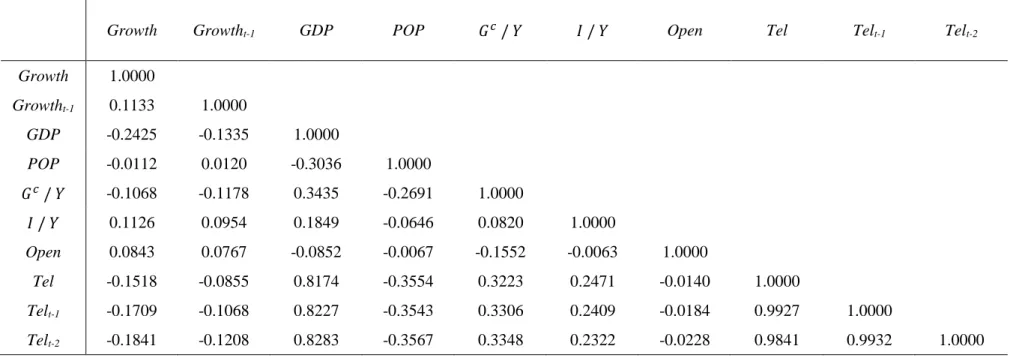
Table VI - Correlation matrix for total samples, time period: 2000-2014

Growth Growtht-1 GDP POP 𝐺𝑐 / 𝑌 𝐼 / 𝑌 Open Tel Telt-1 Telt-2

Growth 1.0000 Growtht-1 0.1133 1.0000 GDP -0.2425 -0.1335 1.0000 POP -0.0112 0.0120 -0.3036 1.0000 𝐺𝑐 / 𝑌 -0.1068 -0.1178 0.3435 -0.2691 1.0000 𝐼 / 𝑌 0.1126 0.0954 0.1849 -0.0646 0.0820 1.0000 Open 0.0843 0.0767 -0.0852 -0.0067 -0.1552 -0.0063 1.0000 Tel -0.1518 -0.0855 0.8174 -0.3554 0.3223 0.2471 -0.0140 1.0000 Telt-1 -0.1709 -0.1068 0.8227 -0.3543 0.3306 0.2409 -0.0184 0.9927 1.0000 Telt-2 -0.1841 -0.1208 0.8283 -0.3567 0.3348 0.2322 -0.0228 0.9841 0.9932 1.0000

Table VII – Summary of results of estimation of equation (5), where Tel t

Growth World Africa Americas Europe Asia & Oceania High Income Upper M. Income Lower M. Income Low Income Developed Less Developed Growtht-1 0.116*** (0.330) 0.153** (0.072) 0.038 (0.058) 0.188*** (0.044) -0.005 (0.089) 0.107** (0.046) 0.136* (0.081) 0.044 (0.062) 0.306** (0.140) 0.253*** (0.057) 0.113** (0.049) GDPt-1 -0.038*** (0.004) -0.102*** (0.015) -0.033*** (0.010) -0.058*** (0.008) -0.035*** (0.007) -0.058*** (0.007) -0.089*** (0.010) -0.062*** (0.014) -0.155*** (0.041) -0.081*** (0.011) -0.033*** (0.005) POP _(0.089) 0.008 _(0.615) 0.493 -4.534*** _{(1.674) (0.214)} -0.148 -0.347** _{(0.156) (0.250)} -0.287 _(0.503) -0.400 _(0.901) 0.388 _(1.753) 0.463 _(0.168) 0.048 _(0.361) -0.110 𝐺𝑐/𝑌 -0.060*** _(0.010) -0.045*** _(0.016) -0.092*** _{(0.024) (0.040)} -0.049 -0.113*** _(0.021) -0.099*** _(0.015) -0.045*** _(0.014) -0.090*** _{(0.026) (0.015)} 0.016 _(0.020) 0.003 -0.058*** _(0.014) 𝐼/𝑌 _(0.007) -0.004 _(0.022) -0.015 _(0.017) 0.006 0.043*** _{(0.015) (0.012)} -0.013 _(0.008) 0.006 _(0.013) -0.016 0.032** _{(0.016) (0.012)} -0.007 0.033*** _{(0.007) (0.009)} -0.004 Open _(0.010) -0.001 _(0.019) -0.020 -0.042* _(0.023) 0.058*** _{(0.015) (0.010)} -0.003 _(0.010) 0.018* -0.030** _(0.015) -0.026* _{(0.013) (0.022)} 0.031 0.033*** _{(0.008) (0.013)} -0.011 Telt 0.018*** (0.003) 0.036*** (0.006) 0.022*** (0.008) 0.044*** (0.010) 0.019*** (0.004) 0.061*** (0.013) 0.066*** (0.009) 0.026*** (0.006) 0.030*** (0.010) 0.079*** (0.015) 0.015*** (0.003) Wald chi2 Prob>chi2 204.98 0.000 77.75 0.000 112.23 0.000 182.10 0.000 145.66 0.000 315.36 0.000 187.49 0.000 57.60 0.000 28.30 0.000 268.31 0.000 148.72 0.000 AR (1) 0.000 0.005 0.019 0.004 0.037 0.019 0.020 0.026 0.036 0.002 0.000 AR (2) 0.415 0.317 0.347 0.108 0.130 0.623 0.530 0.605 0.275 0.102 0.728 Hansen-J 0.863 0.480 0.322 0.143 0.654 0.168 0.641 0.948 0.357 0.515 0.205 Countries 150 43 31 42 34 49 42 35 24 39 111 Obs. 1950 559 403 546 442 637 546 455 312 507 1443