Comparative study of particle size distribution analysis by laser diffraction between dry and liquid dispersion methods

(1)

September, 2017

Ana Sofia Mendonça Cortes

[Nome completo do autor]

Bachelor in Chemical and Biochemical Engineering

[Habilitações Académicas] [Habilitações Académicas] [Habilitações Académicas] [Habilitações Académicas] [Habilitações Académicas] [Habilitações Académicas] [Habilitações Académicas]

Comparative study of particle size distribution

analysis by laser diffraction between dry and liquid

dispersion methods

[Título da Tese]

Dissertation submitted in fulfilment of requirements for degree of Master in

Chemical and Biochemical Engineering

Dissertação para obtenção do Grau de Mestre em

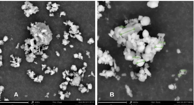
[Engenharia Informática]

Advisor: Dr. Sérgio Silva, Scientist

– Particle Engineering, Hovione

Farmaciencia, SA

Co-advisor: Dr. Mário Eusébio, Assistant Professor, Faculdade de

Ciências e Tecnologias – Universidade Nova de Lisboa

Jury:

President: Dr. Susana Filipe Barreiros

Arguer: Dr. Ana Isabel Nobre Martins Aguiar de Oliveira Ricardo Member: Dr. Sérgio Manuel Campos da Silva

(2)

(3)

I

Ana Sofia Mendonça Cortes

[Nome completo do autor]

Bachelor in Chemical and Biochemical Engineering

[Habilitações Académicas] [Habilitações Académicas] [Habilitações Académicas] [Habilitações Académicas] [Habilitações Académicas] [Habilitações Académicas] [Habilitações Académicas]

Comparative study of particle size distribution

analysis by laser diffraction between dry and liquid

dispersion methods

[Título da Tese]

Dissertation submitted in fulfilment of requirements for degree of Master in

Chemical and Biochemical Engineering

Dissertação para obtenção do Grau de Mestre em

[Engenharia Informática]

Advisor: Dr. Sérgio Silva, Scientist

– Particle Engineering, Hovione

Farmaciencia, SA

Co-advisor: Dr. Mário Eusébio, Assistant Professor, Faculdade de

Ciências e Tecnologias – Universidade Nova de Lisboa

Jury:

President: Dr. Susana Filipe Barreiros

Arguer: Dr. Ana Isabel Nobre Martins Aguiar de Oliveira Ricardo Member: Dr. Sérgio Manuel Campos da Silva

(4)

(5)

III

Comparative study of particle size distribution analysis by laser diffraction between dry and liquid dispersion methods

A Faculdade de Ciências e Tecnologia e a Universidade Nova de Lisboa têm o direito, perpétuo e sem limites geográficos, de arquivar e publicar esta dissertação através de exemplares impressos reproduzidos em papel ou de forma digital, ou por qualquer outro meio conhecido ou que venha a ser inventado, e de a divulgar através de repositórios científicos e de admitir a sua cópia e distribuição com objetivos educacionais ou de investigação, não comerciais, desde que seja dado crédito ao autor e editor.

Faculdade de Ciências e Tecnologia and Universidade Nova de Lisboa have the perpetual right with no geographical boundaries, to archive and publish this dissertation through printed copies reproduced in paper or digital form, or by any means known or to be invented, and to divulge through scientific repositories and admit its copy and distribution for educational purposes or research, non-commercial, as long as the credit is given to the author and Publisher.

(6)

(7)

V

(8)

(9)

VII

Acknowledgements

I would first like to thank Dr. Rafael Antunes and his team for receiving me and teach me along the way, especially my thesis advisor Dr. Sérgio Silva, that supported and guided me throughout this study. Thank you for listening to my opinions and have them in consideration.

I would also like to thank all my laboratory colleagues that made it possible to have fun and learn at the same time, especially, Claúdia Fernandes and Pedro Dinis, who were always ready to answer my questions and teach me something new. For trying to help me with my analytical problems, thank you, Joana Fernandes and Célia Fonseca.

Thank you to all the people from different departments whom I got to know during my internship, that were always ready to help.

Lastly, but not least, thank you to all my family and close friends whom always supported and encouraged me to stay strong and not give up.

(10)

(11)

IX

Abstract

Particle size is an important variable, especially in the pharmaceutical industry, since this is one of the parameters that can influence medicines performance.

Drugs can be administered by different routes of administration and in different dosage forms. The active products analyzed in this study are characterized as inhalation products to be administered as dry powder inhalers.

This type of active product is characterized by particles between 1 μm and 5 μm. Particles in this diameter range can travel through the lungs to the bronchi and alveoli area, where they settle by sedimentation. The performance of these dosage forms is compromised if the API does not meet the specifications regarding particle size.

Two techniques based on laser diffraction were used to determine the particle size distribution of several active pharmaceutical ingredients. Both work under the same principles, however, over the last 20 - 30 years, they have evolved differently. They present two major differences: the mathematical algorithm and the means of dispersion of the particles.

Two types of equipment were used for this type of analysis: Malvern Mastersizer Hydro 2000 S and Sympatec (consisting of Helos, Rodos / M and Aspiros units) for the liquid and dry dispersion, respectively. To verify the accuracy of the results an electronic microscope, the Phenom ProX Generation 5, was used.

After all the analyses and the comparison of the results it was observed that it is possible to obtain similar results of particle size distribution with different techniques. However, this is only verified if the analysis method of both equipments allow a complete particle deagglomeration.

In this study, due to the inherent characteristics of the products and the limits of the equipment, difficulties appeared and made the particle deagglomeration process difficult.

(12)

(13)

XI

Resumo

O tamanho das partículas é uma variável importante, especialmente na indústria farmacêutica, sendo que este é um dos parâmetros que pode influenciar a eficácia dos medicamentos.

Os medicamentos podem ser administrados através de diferentes vias e em diferentes formas farmacêuticas. Os produtos ativos analisados neste estudo são caraterizados como produtos de inalação para serem administrados através de inaladores de pós secos.

Este tipo de produto ativo é caracterizado por partículas entre os 1 µm e 5 µm. Partículas nesta gama de diâmetro conseguem percorrer os pulmões até à zona dos brônquios e alvéolos, nos quais se depositam por sedimentação. Se o produto ativo não estiver de acordo com as especificações, um dos parâmetros afetados será a sua eficácia que diminuirá.

Para averiguar a distribuição do tamanho das partículas foram usadas duas técnicas que têm por base a difração a laser. Ambas têm o mesmo fundamento, no entanto, ao longo dos últimos 20 - 30 anos, evoluíram de forma distinta. Elas apresentam duas grandes diferenças: o algoritmo matemático e o meio de dispersão das partículas.

Foram usados dois equipamentos para este tipo de análises: Malvern Mastersizer Hydro 2000 S e o Sympatec (constituído pelas unidades Helos, Rodos/M e Aspiros) para a dispersão líquida e seca, respetivamente. Para verificar a veracidade dos resultados foi usado um microscópio eletrónico, o Phenom ProX Generation 5.

Após as análises e a comparação dos resultados foi possível verificar que através de diferentes equipamentos é possível obter resultados semelhantes no que diz respeito à distribuição de tamanhos das partículas. No entanto, isto só é verificado se os métodos de análise de ambos equipamentos possibilitarem uma desagregação total das partículas.

Neste estudo, devido às caraterísticas inerentes dos produtos e limites dos equipamentos, dificuldades surgiram que dificultaram o processo de desagregação das partículas.

Palavras-chave: tamanho de partículas, difração a laser, dispersão líquida, dispersão seca

(14)

(15)

XIII

List of figures

Figure 1-1 Particle size range general requirements for different dosage forms and routes of administration [6] ... 1

Figure 1-2 Example of particle shape: spherical particle (left) and irregular particle (right) [5] ... 2

Figure 1-3 Percentiles reported: d(0.1), d(0.5) and d(0.9) [5] ... 3 Figure 1-4 Equation for span parameter ... 4 Figure 1-5 Scattering angle of large particles (above) and small particles (below) [12] 5 Figure 1-6 Diffraction pattern of a small particle (left) and a large particle (right) [13] .. 5 Figure 1-7 Diffraction patterns of non-spherical particles [13] ... 6 Figure 1-8 Schematic of a scanning electron microscope [18] ... 7 Figure 2-1 Desktop scanning electron microscope (SEM) Phenom ProX Generation 5 [15] ... 10

Figure 2-2 Phenom sample holder (left); stub pins (right) ... 10 Figure 2-3 Malvern Mastersizer (back) Hydro 2000 S (front) ... 11 Figure 2-4 Sympatec equipment :Helos (right), Rodos/M (middle) and Aspiros (left) . 12 Figure 2-5 Sample vials for MALVERN (left) and SYMPATEC (right) ... 13 Figure 3-1 APIs nomenclature (example) ... 14 Figure 3-2 Spray dried product after micronization with magnification 4000x and 8000x with 10 kV - Point [06IH13c.SCS038.P6SS] ... 15

Figure 3-3 Table results (3 analyses plus average) on liquid dispersion [06IH13c.SCS038.P6SS] ... 16

Figure 3-4 Normal distribution obtained through liquid dispersion [06IH13c.SCS038.P6SS] ... 16

Figure 3-5 Analysis results on dry dispersion [06IH13c.SCS048.P6SS] ... 17 Figure 3-6 A. Powder sample of unmicronized material at magnification of 4000x - 15kV - Point [06ST71.CFC4340.SS] B. Image of ST71c at magnification 4000x - 10 kV - Point [06ST71c.SCS042.P5SS] ... 18

Figure 3-7 A. Image of ST71c at magnification 6000x - 15 kV - Point [06ST71c.SCS043.P1SS] B. Image of ST71c at magnification 8000x - 15 kV - Point [06ST71c.SCS044.P2SS] ... 19

Figure 3-8 Table results of the average value of liquid dispersion for unmicronized material [06ST71.CFC4340/SS] and three batches [06ST71c.SCS042.P5SS] [06ST71c.SCS043.P1SS] [06ST71c.SCS044.P2SS] ... 20

(18)

XVI

Figure 3-9 Comparison of normal distribution obtained through liquid dispersion between the unmicronized material [06ST71.CFC4340.SS] and the three distinct batches [06ST71c.SCS042.P5SS] [06ST71c.SCS043.P1SS] [06ST71c.SCS044.P2SS]. ... 21

Figure 3-10 Table results on dry dispersion for unmicronized material [06ST71.CFC4340/SS] and three micronized batches [06St71c.SCS042.P5SS] [06ST71c.SCS043.P1SS] [06ST71c.SCS044.P2SS] ... 21

Figure 3-11 Comparison of normal distribution obtained through dry dispersion between the unmicronized material [06ST71.CFC4340.SS] and the three different batches [06ST71c.SCS042.P5SS] [06ST71c.SCS043.P1SS] [06ST71c.SCS044.P2SS]. ... 22

Figure 3-12 A. Powder sample of unmicronized material at magnification of 410x - 15kV - Point [06ST75046.GML9612] B. Image of ST75c at magnification of 6000x - 15 kV - Point [06ST75c.SCS048.P4SS] ... 24

Figure 3-13 A. Image of ST75c at magnification of 6000x - 15 kV - Point [06ST75c.SCS048.P14SS] B. Image of ST75c at magnification of 6000x - 15 kV - Point [06ST75c.SCS048.P15SS] ... 25

Figure 3-14 Table results of the average value on liquid dispersion for unmicronized material [06ST75.GML9612] and three different micronized fractions of SCS048 batch [06ST75c.SCS048.P4SS] [06ST75c.SCS048.P14SS] [06ST75c.SCS048.P15SS] ... 26

Figure 3-15 Comparison of normal distribution obtained through liquid dispersion between the unmicronized material [06ST75046.GML9612] and the fractions of batch SCS048 [06ST75c.SCS048.P4SS] [06ST75c.SCS048.P14SS] [06ST75c.SCS048.P15SS]. ... 27

Figure 3-16 Table results of the average value on dry dispersion for unmicronized material [06ST75.GML9612] and three different micronized fractions of SCS048 batch [06ST75c.SCS048.P4SS] [06ST75c.SCS048.P14SS] [06ST75c.SCS048.P15SS] ... 28

Figure 3-17 Comparison of normal distribution obtained through dry dispersion between the unmicronized material [06ST775046.GML9612] and the three different fractions from batch SCS048 [06ST75c.SCS048.P4SS] [06ST75c.SCS048.P14SS] [06ST75c.SCS048P15SS]. .... 28

Figure 3-18 A. Powder sample of unmicronized material at magnification of 500x - 15kV - Point [05ST75.HQ00072] B. Image of ST75c at magnification of 12500x - 15 kV - Point [06ST75c.SCS050.P6SS] ... 30

Figure 3-19 Table results of the average value on liquid dispersion for unmicronized material [05ST75.HQ00072] and micronized fraction of SCS050 batch [06ST75c.SCS050.P6SS] ... 31 Figure 3-20 Comparison of normal distribution obtained through liquid dispersion between the unmicronized material [05ST75.HQ00072] and the fraction from batch SCS050 [06ST75c.SCS050.P6SS] ... 31

Figure 3-21 Table results of the average value on dry dispersion for unmicronized material [05ST75.HQ00072] and micronized fraction of SCS050 batch [06ST75c.SCS050.P6SS] ... 32 Figure 3-22 Comparison of normal distribution obtained through dry dispersion between the unmicronized material [05ST75.HQ00072] and the fraction attained [P6SS]. ... 32

Figure 3-23 A. Image of ST75c at magnification of 8000x - 15 kV - Point [06ST75c.SCS051.P2SS] B. Image of ST75c at magnification of 8000x - 15 kV - Point [06ST75c.SCS051.P4SS] ... 34

(19)

XVII

Figure 3-24 Images of ST75c at magnification of 8000x - 15 kV - Point – Different sections [06ST75c.SCS051.P5SS] ... 35

Figure 3-25 Table results of the average value on liquid dispersion for unmicronized material [05ST75.HQ00072] and three different micronized fractions of batch SCS051 [06ST75c.SCS051.P2SS] [06ST75c.SCS051.P4SS] [06ST75c.SCS051.P5SS] ... 35

Figure 3-26 Comparison of normal distribution obtained through liquid dispersion between the unmicronized material [05ST75.HQ00072] and three fractions from batch SCS051 [06ST75c.SCS051.P2SS] [06ST75c.SCS051.P4SS] [06ST7c.SCS051.P5SS]. ... 36

Figure 3-27 Table results of the average value on dry dispersion for unmicronized material [05ST75.HQ00072] and two different micronized fractions of batch SCS051 [06ST75c.SCS051.P2SS] [06ST75c.SCS051.P4SS] ... 36

Figure 3-28 Comparison of normal distribution obtained through dry dispersion between the unmicronized material [05ST75.HQ00072] and two fractions from batch SCS051 [06ST75c.SCS051.P2SS] [06ST75c.SCS051.P4SS]. ... 37

Figure 3-29 A. Images of ST75c at magnification of 8000x - 15 kV - Point [06ST75c.SCS052.P5SS] B. Images of ST75c at magnification of 8000x - 15 kV - Point [06ST75c.SCS052.P6SS] ... 39

Figure 3-30 Table results of the average value on liquid dispersion for unmicronized material [05ST75.HQ00072] and four fractions from batch SCS052 [06ST75c.SCS052.P2SS] [06ST75c.SCS052.P3SS] [06ST75c.SCS052.P5SS] [06ST75c.SCS052.P6SS] ... 40

Figure 3-31 Comparison of normal distribution obtained through liquid dispersion between the unmicronized material [05ST75.HQ00072] and four fractions from batch SCS052 [06ST75c.SCS052.P2SS] [06ST75c.SCS052.P3SS] [06ST75c.SCS052.P5SS] [06ST75c.SCS052.P6SS] ... 40

Figure 3-32 Table results of the average value on dry dispersion for unmicronized material [05ST75.HQ00072] and the last fraction from batch SCS052 [06ST75c.SCS052.P6SS] ... 41 Figure 3-33 Comparison of normal distribution obtained through dry dispersion between the unmicronized material [05ST75.HQ00072] and the fraction from batch SCS052 [06ST75c.SCS052.P6SS]. ... 41

Figure A-1 Trend graphs for d(0.5) at different US percentage: A 30% ultrasounds; B 50% ultrasounds; C 80% ultrasounds [IH13c method development] ... 55

Figure A-2 Adjustment of parameters: refractive index and absorption. Before (above) and after (below) [IH13c method development] ... 56

Figure A-3 Titration curve: pressure [IH13c method development] ... 58 Figure A-4 Powder sample of unmicronized material [06ST71.CFC4340.SS] at 15kV – Point and magnification of: 500x (A), 1000x (B and C – Different sections) and 2500x (D) ... 60

Figure A-5 Titration curves for unmicronized material [06ST71.CFC4340.SS] : pressure (above) and feed rate velocity (below) [ST71c method development] ... 62

Figure A-6 Titration curves for micronized material : pressure [ST71c method development] ... 63

(20)

XVIII

Figure A-7 Titration curves for micronized material: feed rate velocity (below) [ST71c method development] ... 64

Figure A-8 Titration curves for unmicronized material [06ST75046.GML9612] : pressure (above) and feed rate velocity (below) [ST75c method development] ... 66

Figure A-9 Titration curve for micronized material [06ST75c.SCS048.P4SS]: pressure [ST75c method development] ... 67

Figure A-10 Titration curve for micronized material [06ST75c.SCS048.P15SS]: pressure (above) and feed rate velocity (below) [ST75c method development] ... 68

Figure A-11 Titration curves for micronized fraction 06ST75.SCS050.P6SS : pressure (above) and feed rate velocity (below) [ST75c method development] ... 70

Figure A-12 Titration curves for micronized fractions from 06ST75.SCS051 batch : pressure (above) and feed rate velocity (below) [ST75c method development] ... 72

Figure A-13 Titration curves for micronized fraction 06ST75.SCS52.P6SS: pressure (above) and feed rate velocity (below) [ST75c method development] ... 74

(21)

XIX

List of tables

Table 1-1 Definition of the reported percentiles ... 3

Table 1-2 Parameters to be evaluated [MALVERN] [22] ... 8

Table 1-3 Reccomended obscuration ranges dependent on particle size [22] ... 8

Table 2-1 Dispersant and surfactant list [MALVERN] ... 11

Table 2-2 Lens range [SYMPATEC] ... 13

Table 3-1 Analytical conditions on liquid dispersion for solid powders for product [IH13c] ... 16

Table 3-2 PSD results obtained from liquid dispersion vs dry dispersion analyses for [06IH3c] ... 17

Table 3-3 Analytical conditions on liquid dispersion for solid powders for product [ST71c] ... 20

Table 3-4 PSD results obtained from liquid dispersion vs dry dispersion analyses for [06ST71c] ... 23

Table 3-5 Analytical conditions on liquid dispersion for solid powders for product [ST75c] ... 26

Table 3-6 PSD results obtained from liquid dispersion vs dry dispersion analyses for [06ST75c.SCS048] ... 29

Table 3-7 PSD results obtained from liquid dispersion vs dry dispersion analyses for [ST75c.SCS050] ... 33

Table A-1 Equipment specification: Phenom ProX ... 50

Table A-2 Equipment specification: Malvern Hydro 2000 S ... 50

Table A-3 Equipment specification: Sympatec Helos ... 51

Table A-4 Equipment specification: Sympatec Rodos/M ... 52

Table A-5 Equipment specification: Sympatec Aspiros ... 52

Table A-6 Dispersant/surfactant test [IH13c method development] ... 54

(22)

(23)

XXI

Glossary

Excipients = also known as inactive ingredients, they are agents that combine with active ingredients to facilitate drug transport in the body [1].

Potency = is a measure of drug activity expressed in terms of the amount required to produce an effect of given intensity [2].

Potent APIs = a pharmacologically active ingredient or intermediate with biological activity at approximately 15 µm/kg of body weight or below in humans. Characterized with high selectivity and/or potential to cause cancer, mutations development effects or reproductive toxicity at low doses [3].

(24)

(25)

XXIII

Acronyms

API = Active Pharmaceutical Ingredient EDS = Energy Dispersive Spectroscopy

MALVERN = MALVERN Mastersizer HYDRO 2000S nm = nanometers

PS = Particle Size

PSD = Particle Size Distribution RN = Record Number

SEM = Scanning Electron Microscope (Phenom ProX) SYMPATEC = HELOS + RODOS/M + ASPIROS US = ultrasounds

(26)

(27)

1

Chapter 1 __________________Introduction

1.1 Analysis of Particle Size

Particle size influences many properties of particulate materials and is a valuable indicator of quality and performance. Particle size can also influence a large variety of important physical properties, manufacturing processability and quality attributes. Some examples are dose uniformity, aerosolization behavior and performance [6].

Considering particulate materials, the particle size distribution (PSD) is an important parameter to analyze. PSD requirements of materials depend on the industry and on the materials’ final use. For instance, in paint and pigment industries, it is important that the PSD is within specified limits or else it may influence the gloss appearance. The shape and size of glass beads may affect the reflectivity of the highway paints, if PSD is not within the specifications. Another example can be found in the food industry where the PSD of chocolate powders impacts its flavor and color [5].

The PSD is undoubtedly important in diverse industries [5].

In the pharmaceutical field, drug substances and dosage forms can be highly affected by the particle size, therefore PSD is a critical process parameter in pharmaceutical production [6]. For example, the particle size and shape may affect the dissolution rate and bioavailability of active pharmaceutical ingredients, as well as the drug release rate for sustained and controlled release formulations [6].

Figure 1-1 Particle size range general requirements for different dosage forms and routes of administration [6]

In Figure 1-1, it is presented the variety of ideal particle size (PS) ranges for different dosage forms, depending on the routes of administration [6]. Different routes of administration will have different particle size limitations to obtain an ideal performance.

(28)

2

The particle size distribution and shape of the delivered dose is more critical for inhalation than most of the other conventional drug products because these factors greatly influence the deposition profile in the lungs of the patient [7].

This study is focused on APIs (active pharmaceutical ingredients), designed for dry powder inhalers, which means that they must be designed to have an aerodynamic diameter less than 5 µm, to be suitable for respiratory delivery [8]. The optimum aerodynamic particle size distribution for most inhalation aerosols has generally been recognized as being in the range of 1 – 5 µm [5-6]. If the particles are within this range, they can deposit themselves in the bronchial and alveolar regions predominantly by sedimentation, and have the best pulmonary penetration [6].

The particle size will not only greatly vary with the dosage form or route of administration, but also with the place where it must deposit to achieve an optimum response.

APIs are formulated with excipients, so that they can be dispersed into their primary respiratory size upon inhalation through dry powders inhalers [8]. Normally, this type of inhalers contain an active ingredient and one or more excipient to aid powder dispersion and flow [7].

In pulmonary delivery of pharmaceuticals, the particle size distribution is the most important parameter affecting the formulation performance [6].

In the scope of this study and the measurement range of the particles (nanometers), a particle can be described as a 3-dimensional object, which unless a perfect sphere, it cannot be fully described by a single dimension such as diameter [4]. To describe the size of a particle it is used the spherical form as a reference. In other words, it is determined the spherical equivalent diameter and that way it is possible to evaluate every particle equally [3-4].

Since the spherical shape is the only shape that can be described as one measurement, using the spherical equivalent diameter makes comparing results easier between analyses.

As mentioned, if the particle is spherical, the diameter is used to describe the particle. However, when the particle has an irregular shape, depending on the direction it is measured, vertically or horizontally, for instance, the diameter is going to have different dimensions (Figure 1-2) [5].

Figure 1-2 Example of particle shape: spherical particle (left) and irregular particle (right) [5]

To describe an irregular particle, it is necessary to have multiple lengths and widths to provide a measurement with a good accuracy. To simplify, many PSD techniques make the assumption that every particle is spherical, being the reported value the equivalent diameter [4]. It is conveyed that this assumption has no impact in most products, however, that may change with particles with large aspect ratio such as needle shaped particles.

(29)

3

The results can be presented in diverse ways or types of distributions, for example: weighted, number weighted, volume weighted or intensity weighted [4]. Usually, they are represented by a frequency or a cumulative distribution curve [9].

Although there are different types of distributions that can be used to display PS results, equipments that use techniques such as laser diffraction, will present the results as a volume weighted distribution [3-4]. This is often useful from a commercial perspective as the distribution represents the composition of the sample as volume per mass, and therefore its potential monetary value [4].

The volume weighted distribution is more used than the others mentioned. However, it is important to know that if samples are being compared or re-analyzed, they must be done with the same technique, because if not, they cannot be compared, since the results will be too different due to the different calculation mechanism [4].

However, if needed, it is possible to convert the results for the number weighted distribution, for instance, but that will increase greatly the number of errors induced [5].

When using the volume weighted distribution, it is common to have the results displayed based on the maximum particle size for a given percentage of the sample, in which the most common percentiles reported are Dv10, Dv50 and Dv90 [4].

Table 1-1 Definition of the reported percentiles

D Diameter

v Volume weighted distribution

10, 50, 90 Percentage of sample below this particle size (it can be written in decimal fraction)

In this study Dv10, Dv50 and Dv90 will be the percentiles reported, however, they will be written as d(0.1), d(0.5) and d(0.9).The v can be dropped because if omitted, the assumed distribution shall be the volume weighted since it is the most commonly used.

In Figure 1-3 it is possible to observe the percentiles d(0.1) and d(0.9) on a distribution, as well as the median which is represented by d(0.5) [5].

(30)

4

Using the percentiles d(0.1), d(0.5) and d(0.9) it is possible to calculate another PSD parameter: span. The span is calculated as shown in the equation from Figure 1-4.

Figure 1-4 Equation for span parameter

Span parameter is important to understand if the particle size range is wide or narrow [5]. If the span value is high (for example, higher than 2) it is probable that the distribution has two distinct populations regarding the PS. Typically a PSD with span higher than 2 displays two distinct populations, one of fine particles and other of larger particles. Usually, a normal (gaussian) distribution has a span between 1 and 2.

1.2 Methods to Measure Particle Size

When analyzing a new product, it is necessary to assess all possible parameters such as particle size and shape, surface and mechanical properties, so that we get all the information needed for later analyses and/or for interpreting the results obtained [4]. The particle size can be measured by different methods in different conditions, usually, dry or wet.

For the techniques per se, in this study, they are focused solely on two: image analysis for SEM and laser diffraction using both MALVERN (Malvern Mastersizer HYDRO 2000S) and SYMPATEC (Symptec HELOS, RODOS/M and ASPIROS). The main difference between the two last mentioned, is the particle size calculation algorithm and the mechanism of the equipment. However, the original concept behind is similar.

The SEM works almost like an optical microscope but with a greater range. However, by itself, it is not enough to determine the PSD of a sample. Errors can be induced, especially if the sampling is not well executed [4], because it will mean that what is being observed is not the reality of the bulk and this will lead to incorrect results. However, this is a common problem to all techniques.

It is imperative not to use the SEM alone, but with other techniques as executed in this study, not only to get a closer and an actual PSD, but to ensure that the PS method used by other techniques is correct and accurate since errors can be induced through different sources.

Each of the equipments used in this study have an analytical method to follow. MALVERNs method is stricter than SYMPATECs in the way that is always the same for the same product, since it is valid for a limited range of PS. However, with SYMPATEC, even with the same product, if the PS of the batch is different, probably, new conditions must be studied to achieve a good dispersion for the analyses.

For MALVERN and SYMPATEC, PS is determined by laser diffraction. This technology has been used in the last 20 – 30 years and it has been optimized throughout the years resulting in a well-established technique that it is the standard technology and widely used in the pharmaceutical industry [6, 10].

With laser diffraction methods, it is possible to have fast analyses (usually less than a minute), wide measurement range, high precision, reproducibility, instant feedback and low maintenance [6, 10]. Another strong point is that the sample can be analyzed in both states, liquid or solid [10].

𝑆𝑝𝑎𝑛 = 𝑑 0.9 − 𝑑(0.1) 𝑑(0.5)

(31)

5

The determination of PS using laser diffraction technique is based on the angular variation in the intensity of the light scattered as a laser beam passes through a dispersed particulate sample, as can be observed in Figure 1-5 [4, 11].

Figure 1-5 Scattering angle of large particles (above) and small particles (below) [12]

Figure 1-6 Diffraction pattern of a small particle (left) and a large particle (right) [13]

The effect of the laser beam is different depending on the size of the particles in the sample. Smaller particles scatter the light at larger angles while large particles scatter the light at smaller angles [12]. This can be demonstrated through both Figure 1-5 and Figure 1-6.

After analyzing the angular intensity data, it is possible to calculate the PS of the particles responsible for the scattering patterns applying the Mie or the Fraunhofer diffraction theories [4].

Both consist of mathematical expressions that use the input information to originate the link between both variables, angular intensity and particle size. These theories are used to calculate what kind of light intensity distribution patterns are produced by particles of various sizes, and this data is stored beforehand on a computer as a parameter table (numerical table) containing a vast amount of information [14].

(32)

6

A considerable amount of time is required for calculating this parameter table. However, in actual measurement of PSD, the measurement time is not affected since there are parameters tables already calculated and stored in computer memory [14].

Both theories are based on the same principle. However, since the Fraunhofer is a simplified version of the Mie theory, it cannot be used without restrictions, that will lead to errors. Because of that, normally, two conditions must be satisfied [14]:

1. The particle size must be relatively large (at least 10 times bigger than the laser wavelength)

2. Small scattering angle (30º or less) must be observed.

Because of the above-mentioned requirements, this theory is not applicable for measurements in the sub-micron region. This theory was especially used when the computers could not be fast enough to decode the complex programming that the Mie theory requires. Nowadays, due to the technological evolution, the latter is mostly applied. The only exception occurs when the PS is extremely large. In those cases Fraunhofer diffraction theory is used to avoid calculation error building up that can occur with the Mie theory [14].

Figure 1-7 Diffraction patterns of non-spherical particles [13]

However, if the sample particles are not spherical, but they are instead more irregularly shaped, as seen in the Figure 1-7, the pattern acquired is different. The further away the particles are from the spherical shape, more differences the pattern will have.

The presence of irregular shapes is one of the major difficulties this technique faces that may induce to major errors, but it is not the only one. Aggregation is another problem that can happen and may difficult the analyses.

Companies research different methods and try diverse algorithms to have exact analyses’ results, resulting in a wide-range of analytical instruments.

1.2.1 Scanning Electron Microscopy

Desktop scanning electron microscopes (SEM) are considered a high-performance SEM for imaging and analysis [15].

(33)

7

The SEMs provide excellent imaging due to the high brightness and long-life electron source, as well as fast SEM imaging with high resolution. There are several models to fit the diverse application needs. They are user friendly equipments with low maintenance required [16].

One of the most significant differences between a modern light microscope and a SEM is the magnification range. In a light microscope, the maximum magnification a microscope can reach is limited not only by the number and quality of the lenses, but especially by the wavelength of the light used as illumination source. These microscopes usually have a maximum magnification of approximately 1000x due to the limitations that the white light wavelength has (400 nm to 700 nm) [17].

To have higher resolution on higher magnifications, electrons started to be used, since they have shorter wavelengths.

To be able to scan the sample, first, the electrons are produced at the top of the column, which then will travel down through diverse lenses and openings to produce a beam of electrons. The beam will hit the sample mounted on the chamber area which should be under vacuum. Due to the presence of scan coils above the lens, it is possible to scan different areas of the sample. In Figure 1-8, it is shown a diagram of a SEM mechanism [18].

Figure 1-8 Schematic of a scanning electron microscope [18]

Due to the interaction between the electrons and the sample, secondary electrons and backscattered electrons are emitted along with characteristic X-rays. These secondary electrons after being collected by detectors, form images that are then displayed on the computer screen with help of the software [18-19]

Generally, SEM is considered a nondestructive technique, even though in the case of some more sensitive products, sample degradation may occur.

The SEM technique has a wide range of applications and is used by different industries in the pharmaceutical and medical fields providing imaging analysis and EDS (Energy-dispersive X-ray spectroscopy) [21].

(34)

8 1.2.2 Laser Diffraction with Wet Dispersion

The analysis of particles size using laser diffraction method is often performed using MALVERN equipments. With this equipment it is possible to analyze the particle size dry or wet, but the process to do it is not as straightforward as on the SEM since different factors and parameters must be considered. On a first-time analysis, the analysis conditions are unknown and several tests must be carried out to determine optimal analysis conditions.

In this equipment, the parameters on Table 1-2 should be evaluated.

Table 1-2 Parameters to be evaluated [MALVERN] [22]

Dispersant Must wet the sample, add energy to improve the dispersion, as well as provide stabilization

Sampling The sample quantity must be representative of the bulk Obscuration range Sample concentration read by the laser

Measurement duration Must be long enough to allow a representative sample of the particles to circulate through the measurement cell

Stir speed Must ensure homogeneity and that the sample passing through the measurement cell is representative

All the variables mentioned above may lead to PS determination with errors if not evaluated properly. One of the problems that may affect sample measurement that can originate from the obscuration parameter is the multiple scattering effect. This can happen if the obscuration range being used is not the recommended (although even the same types of particles may react differently) [22].

On Table 1-3 it is possible to see the recommended obscuration ranges for different particle sizes.

Table 1-3 Reccomended obscuration ranges dependent on particle size [22]

Particle Size Obscuration range Fine particles ~5% to 10% (less than 5%

may be required for <1µm)

Coarse particles 5% to 15%

Polydisperse samples 15% to 20%

It is important to mention that fine particles are more easily affected by multiple scattering effects, while coarser particles are more likely to be affected by sampling [22].

As for the laser diffraction technique used to calculate the PSD, the MALVERN uses the Mie theory, which means it requires knowledge of optical properties (refractive index and imaginary component) of the sample and of the dispersant. Typically, when the optical properties are unknown, an estimated value is used, since it is possible to fit the modeled data with the actual collected data with help of the software [23].

The other option available when the optical properties are not known is using the Fraunhofer theory, however, MALVERN does not recommend this approximation if the sample has particles below 50µm or if they are relatively transparent.

1.2.3 Laser Diffraction with Dry Dispersion

The analysis of particles size using laser diffraction method can also be performed using SYMPATEC equipments. This equipment is often composed of independent modules according

(35)

9

to the customer needs. The HELOS (Helium-Neon Laser Optical System) is the main part of the equipment, since it contains the laser. Its measuring range is dependent on which one of the 4 lenses is being used. The measuring range varies from 0.18µm to 875µm [24]. The RODOS/M is then attached to the main part as the dry dispersion unit. It can be used for almost all kinds of dry powders with a PS range of <0.1µm to 3500µm. This component is completely automatic, which means all the parameters are selected from the database in the software. To disperse the particles, the unit uses compressed air that will generate a dry aerosol that will then pass in front of the laser beam. After the analyses, the powders are collected by suction into a vacuum [25]. To have an easy and homogeneous dosing, especially for small quantities or potent products it is recommended to use the ASPIROS accessory. Potent products must be prepared inside a glove box. Vials are filled with a few milligrams of the product and capped. Since the vial is placed inside the ASPIROS accessory, the risk is minimized [26].

The laser diffraction technique used in SYMPATEC equipment is considered a parameter free and a model independent mathematical algorithm, since it does not need the parameters refractive index and imaginary component, like on MALVERN. This was possible with the Philips-Twomey algorithm [27].

The HELOS unit laser can evaluate the PSD with [24]:

▪ FREE (Fraunhofer Enhanced Evaluation) applying the Fraunhofer theory down to 0.1µm. This theory is possible to be applied without knowledge of optical parameters.

▪ MIEE (Mie Extended Evaluation) through the Mie theory which is appropriated for spherical, isotropic, homogeneous particles with known complex refractive index and more.

It is important to mention that the FREE is different from the Fraunhofer theory, since it is the “upgraded” version with the Philips-Twomey algorithm, which is meant to counter the problems associated with the theory.

To summarize, in both equipments (MALVERN and SYMPATEC) a good dispersion must be achieved to obtain correct values of the particle size. Bad dispersions originate misleading PSD values as a result of the formation of the particle aggregates that will shift PSD to higher values.

In this work, whenever it was possible, the samples were analyzed with both the wet method (MALVERN) and the dry method (SYMPATEC). Additionally, product samples were also analyzed by SEM.

All the products analyzed were considered potent by Hovione’s internal procedures. They were categorized with a category 3a, which means that all products were handled by following the requirements and strict procedures [28].

(36)

10

Chapter 2 ___________Materials & Methods

All the equipment used were property of Hovione’s analytical R&D Products laboratory. 2.1 Desktop Scanning Electron Microscope Phenom ProX Generation 5

Figure 2-1 Desktop scanning electron microscope (SEM) Phenom ProX Generation 5 [15]

The Phenom ProX Generation 5 (Figure 2-1) was the SEM used.

The SEM has a simple preparation method and it can only be used to analyze solids. The preparation of samples must be done in a contained environment such as a glove box if it is a potent product, to ensure the protection of the operator.

For the sample preparation, the powder sample is placed on a carbon double sided adhesive tape previously mounted on a clean stub pin. Subsequently the pin is gently sprayed using compressed air to remove the excess powder that did not adhered to the carbon tape.

Afterwards, the stub pin is placed on the phenom sample holder (Figure 2-2). The stub pin must be rotated to lower the sample until 2 mm below the top surface (4 vertical marks) and then placed on the equipment.

Figure 2-2 Phenom sample holder (left); stub pins (right)

Next, captures of the sample at different magnifications are done and measurements of particle size taken manually.

(37)

11 2.2 Malvern Mastersizer Hydro 2000 S

Figure 2-3 Malvern Mastersizer (back) Hydro 2000 S (front)

One of the equipment used for the PSD analyses was a MALVERN Mastersizer Hydro 2000 S (Figure 2-3) which is composed of two separated units: the laser unit (Mastersizer) and the dispersion unit (Hydro 2000 S), which can be replaced by other units depending on the type of analyses to be done.

By connecting the two units together, the laser beam will pass through the dispersed particulate sample on the measurement cell of the dispersion unit, enabling the analyses to happen.

The MALVERN equipment can be used with product in form of suspensions or powders. Before analyzing a new product, a new method must be created following the directions described in Hovione’s Corporate Operating Procedure (COP037) which can be summarized in the steps below. It is advisable to perform a SEM analysis before initiating the method development to determine the measuring range of the PSD.

The first step consists of testing dispersion solutions and surfactants and select the combination that produces a good suspension. The surfactants are chosen based on the polarity of the solvent used during the production of the product and the dispersants available (Table 2-1)

Table 2-1 Dispersant and surfactant list [MALVERN]

Dispersant Surfactant Water Tween 80/20, SDS, IGEPAL Methanol Isopropanol N-hexane Span 85, Lecithin Heptane Isoparaffin

Subsequently, it is necessary to select the sample amount. It is advisable to use 30 to 50 mg, being the minimum limit 20 mg. To be considered representative, at least half of the suspension must be used.

Afterwards, an ultrasounds (US) titration curve for different values of US is done (must be done with independent samples). On this step, the default conditions on the software are

(38)

12

employed. It is considered satisfactory only if the obscuration does not decrease during the analysis.

If the obscuration decreases during the analysis, changes in the default conditions of parameters like stirrer speed, obscuration and/or optical model (refractive index and absorption) must be made or eventually, a new dispersant/surfactant must be tested.

To proceed to the last step a plateau must be reached and the obscuration must remain unchanged. To finalize the method, tests of stability, repeatability and robustness are done.

In the case of an existing validated method the sample preparation and analysis should be performed according to that method. For the analyses to be considered valid, the residual values must be inferior to 2.

The equipment specifications are presented in Appendix I. 2.3 Sympatec Helos, Rodos/M plus Aspiros

Figure 2-4 Sympatec equipment :Helos (right), Rodos/M (middle) and Aspiros (left)

The equipment used was made of three different components: HELOS, RODOS/M plus ASPIROS (Figure 2-4) previously described. The equipment specifications are presented in Appendix I.

With dry samples on SYMPATEC, the method is more linear and simple since only two variables are considered critical.

The variables are pressure, feed rate velocity and density, in which the pressure is usually the most critical parameter. In this work, the only variables studied are the two first mentioned, since the density of the products is unknown, it was used a standard value of 1 g/cm3

for all the products analyzed.

The preparation of the sample is done by filling a glass vial with some milligrams of the powder sample. The quantity required may vary with the product, however, it must be enough to obtain a minimum of 5% of optical concentration.

(39)

13

When analyzing a new product and having previously obtained a SEM image, the next step is to choose the appropriate lens so the analysis is carried out within the range of the lens (Table 2-2).

Table 2-2 Lens range [SYMPATEC]

Lens Range

R1 0.18 µm – 35 µm R2 0.45 µm – 87.5 µm R4 1.80 µm – 350 µm R5 4.50 µm – 875 µm

In case of the analysis of a new product, after selecting the appropriate lens, it should be carried out several tests to determine the optimal velocity values regarding the feeding rate and pressure that provides dispersion without damaging the sample particles.

If the product was previously analyzed and studied, after the vial preparation, it is only needed to place the sample vial inside the sample holder inside the equipment, set the conditions on the software and run the program to obtain the results.

In the Figure 2-5 it is possible to see the differences between the vials of the last two equipments mentioned, MALVERN and SYMPATEC.

(40)

14

Chapter 3 ______________Results and Discussion

The particle size of the different APIs was studied using the thecniques mentioned in chapter 1: SEM, liquid and dry dispersion techniques, Malvern and Sympatec, respectively.

The APIs used in these studies were produced using Hovione’s particle engineering technology wet polishing (WP). Using this technology it is possible to produce stable crystalline APIs with a desired PS in a wet environment, that is isolated by spray drying [29].

Hovione’s internal code for the APIs can be explained with the example on Figure 3-1.

Figure 3-1 APIs nomenclature (example)

In this chapter are presented and discussed the results obtained. Throughout this chapter only results of dry fractions are presented. Meaning that the omitted fractions were analyzed while in suspension (before being feed to the spray dryer) to provide a better understanding of the PSD and in an attempt to maximize the quantity of API to be retrieved.

3.1 IH13c

IH13 is the Hovione’s internal code of specific API intended to be used in a dry powder inhaler. IH13, an inhalation API, was micronized to produce samples with two different and distinct particle size distributions:

i. d(0.5) approximately 3 µm and d(0.9) below 7 µm ii. d(0.5) approximately 4 µm and d(0.9) below 9 µm

(41)

15 3.1.1 SEM

Figure 3-2 obtained by SEM shows oval to circularly shaped particles with variable particle size. Smaller particles are approximately 1 µm in size and the larger ones 5 µm, approximately.

3.1.2 MALVERN vs SYMPATEC

Since IH13 was a new product there was not an existing method for PS determination on MALVERN. The development of the PS method was performed according to the procedure described previously on sub chapter 2.2. It is shown in detailed in Appendix II.

After determining the optimum analysis parameters for dry powders on liquid dispersion as described in Table 3-1, it was possible to proceed with the analysis. The dispersant selected was 0.1 % (w/v) Lecithin in n-heptane.

A

B

Figure 3-2 Spray dried product after micronization with magnification 4000x and 8000x with 10 kV - Point [06IH13c.SCS038.P6SS]

(42)

16

Table 3-1 Analytical conditions on liquid dispersion for solid powders for product [IH13c]

SOLID POWDERS Accessory

Sample handling unit Hydro 2000S

Stirrer speed (rpm) 2100 rpm

Ultrasonic (%) 50 %

Time of ultrasounds 150 seconds

Measurement options Material

Refractive index 1.65

Absorption 0.1

Dispersant name N-heptane

Refractive index of the dispersant agent 1.39 Result calculation

Model General Purpose

Calculation sensitivity Normal sensitivity

Particle shape Irregular

Measurement

Sample measurement time 10 seconds (10000 snaps)

Background measurement time 10 seconds (10000 snaps)

Number of measurements 3

Delay 10 seconds

Average Create average result

Obscuration limits 5 % - 10 %

After the development of the analytical method with the last part of the batch and analyzed, it was achieved the results described in Figure 3-3 and Figure 3-4.

Figure 3-3 Table results (3 analyses plus average) on liquid dispersion [06IH13c.SCS038.P6SS]

The analyses were considered valid because the obscuration values were within the limit proposed and the residual values were inferior to 2.

When comparing the d(0.1), d(0.5) and d(0.9) average values obtained on MALVERN (1.234 / 2.697 / 4.977) with the SEM images, it can be observed that the results are in agreement.

Figure 3-4 Normal distribution obtained through liquid dispersion [06IH13c.SCS038.P6SS]

The Figure 3-4 shows the presence of a fraction of fine powder (particles with PS lower than 1 µm). No turbulence effects were observed during the analysis.

(43)

17

In the case of SYMPATEC analyses (dry dispersion), a method was also developed by studying the pressure and feed rate velocity titration curves of the micronized product (shown in Appendix III). After analyzing and comparing the curves and with the help of SEM images it is possible to establish the ideal conditions for the analysis (1 bar at 36 mm/s), using the lens, R1.

Figure 3-5 Analysis results on dry dispersion [06IH13c.SCS048.P6SS]

The histogram shown in Figure 3-5 is in good agreement with the histogram obtained through liquid dispersion (Figure 3-4). The most obvious difference found was a bigger ratio of fine powders/big particles than in MALVERN analysis, resulting in a higher span and a broader curve.

Table 3-2 PSD results obtained from liquid dispersion vs dry dispersion analyses for [06IH3c]

D (0.1) D (0.5) D (0.9)

MALVERN 1.234 2.697 4.977

SYMPATEC 0.68 2.56 5.84

DIFFERENCE 0.554 0.137 0.863

When comparing the PSD, it can be observed that the SYMPATEC’s sample shows a lower value of d(0.1) and a higher d(0.9), however d(0.5) values were similar in both methods. For this product specifications the d(0.1) is not a critical parameter so the difference between both results is not significant. On the other hand, d(0.9) is critical but the difference is less than 1 µm and both values are still within the limits required by the client (specification i).

On SEM images it is possible to observe particles with a size bigger than 5 µm so we can assume that the probability of d(0.9) from SYMPATEC being closer to the real seem higher than the MALVERN’s d(0.9) values.

3.2 ST71c

ST71 it is the Hovione’s internal code for a steroid API. This product that was micronized to originate batches with two different PS targets, specifically for d(0.5) and d(0.9):

i. d(0.5) approximately 3.5 µm and d(0.9) below 8 µm ii. d(0.5) approximately 4.5 µm and d(0.9) below 10 µm

(44)

18

With the wet polishing method there were 3 different and independent batches obtained (06ST71c.SCS042.P5SS, 06ST71c.SCS043.P1SS and 06ST71c.SCS044.P2SS). The samples from the 3 batches were analyzed by SEM, MALVERN and SYMPATEC.

3.2.1 SEM

Throughout the analysis of the Figure 3-6 A it is possible to see that the unmicronized material does not have a spherical shape but instead an irregular/rectangular shape. Since the unmicronized material does not have a spherical shape we can only say roughly that the measurements have an extended range from 2 µm to 55 µm although the majority appears to be within 15 µm to 20 µm range (more SEM images on Appendix IV).

For the batch 06ST71c.SCS042 (Figure 3-6 B) it is possible to see a clear change in the particle size and shape. After the WP micronization, the particles are smaller but still with irregular outlines. There is a lot of small particles but the majority seems to be between 3 µm to 6 µm.

Figure 3-6 A. Powder sample of unmicronized material at magnification of 4000x - 15kV - Point [06ST71.CFC4340.SS]

B. Image of ST71c at magnification 4000x - 10 kV - Point [06ST71c.SCS042.P5SS]

A

B

(45)

19

The figure above represents the two batches obtained (06ST71c.SCS043.P1SS and 06ST71c.SCS044.P2SS) that complied with the client’s desired specifications regarding the particle size.

The pictures shown in Figure 3-7 seem to be similar between them in appearance with subtle differences since the batches variations are small and the particles irregular.

3.2.2 MALVERN vs SYMPATEC

There was an analytical method validated by Hovione available for PS analyses using MALVERN which was the one used in this study. The optimal analytical conditions used are described in Table 3-3.

The dispersant used was water plus 0.1 mL of surfactant 10% (w/v) of SLS aq. solution.

A

B

Figure 3-7 A. Image of ST71c at magnification 6000x - 15 kV - Point [06ST71c.SCS043.P1SS]

B. Image of ST71c at magnification 8000x - 15 kV - Point [06ST71c.SCS044.P2SS]

(46)

20

Table 3-3 Analytical conditions on liquid dispersion for solid powders for product [ST71c]

SOLID POWDERS Accessory

Ultrasonic (%) 50 %

Absorption 0.1

Dispersant name Water

Measurement

Delay 10 seconds

After preparing the slurry with the samples and with all the information provided, the unmicronized material and three batches were analyzed. The results acquired included several parameters which are shown in Figure 3-8 below.

Figure 3-8 Table results of the average value of liquid dispersion for unmicronized material [06ST71.CFC4340/SS] and three batches [06ST71c.SCS042.P5SS] [06ST71c.SCS043.P1SS]

[06ST71c.SCS044.P2SS]

The analyses were valid since the obscuration is within the range specified and the residual value is lower than 2.

For the unmicronized material, when comparing the results from the liquid dispersion (Figure 3-8 RN4) with the SEM images (Figure 3-6 A) it is possible to observe that the results seem to be in agreement. For the three micronized batches (Figure 3-8 RN32, RN56 and RN60), the PSD shows to be close to each other which is supported by the similar SEM images obtained. On the Figure 3-9 it is possible to compare the PSD evolution from the unmicronized material [06ST71.CFC4340.SS] to the three micronized batches (06ST71c.SCS042.P5SS, 06ST71c.SCS043.P1SS and 06ST71c.SCS044.P2SS).

(47)

21

Figure 3-9 Comparison of normal distribution obtained through liquid dispersion between the unmicronized material [06ST71.CFC4340.SS] and the three distinct batches [06ST71c.SCS042.P5SS]

[06ST71c.SCS043.P1SS] [06ST71c.SCS044.P2SS].

In Figure 3-9, it is possible to see that the unmicronized material distribution shifted more to the left side after micronization. The three micronized batches have identical PS distributions as expected, however, since the two batches with smaller PSD (06ST71c.SCS042.P5SS and 06ST71c.SCS043.P1SS) have a bigger population of fine particles, their histograms seem leaner and more uniform than the last batch (06ST71c.SCS044.P2SS).

ST71c had not been analyzed on dry dispersion before, therefore a new method was developed. A pressure and a feed rate velocity titration curve was done for both the unmicronized material and the micronized products (Appendix V).

By comparing the titration curves with SEM images it was determined the optimum analysis conditions (lent R2, 50 mm/s and 2 bar and lens R1, 50 mm/s and 3 bar for unmicronized material and for micronized product, respectively).

Figure 3-10 Table results on dry dispersion for unmicronized material [06ST71.CFC4340/SS] and three micronized batches [06St71c.SCS042.P5SS] [06ST71c.SCS043.P1SS] [06ST71c.SCS044.P2SS]

From the Figure 3-10 it is possible to distinguish the unmicronized material from the micronized product. By looking at the values of d(0.1), d(0.5) and d(0.9), the discrepancies on the results of the three micronized batches are not as pronounced as in the results on MALVERN with liquid dispersion. In this equipment, the batch 06ST71c.SCS042.P5SS is more similar to the 06St71c.SCS.P2SS than to the 06ST71c.SCS043.P1SS as seen before.

(48)

22

Figure 3-11 Comparison of normal distribution obtained through dry dispersion between the unmicronized material [06ST71.CFC4340.SS] and the three different batches [06ST71c.SCS042.P5SS]

[06ST71c.SCS043.P1SS] [06ST71c.SCS044.P2SS].

As seen in Figure 3-11 and as mentioned before, the unmicronized material PSD histogram is shifted to the left side as the micronization process proceeds. It is possible to see that three micronized batches histograms are quite similar unlike on liquid dispersion.

On SYMPATEC’s histogram it is possible to see small variations between the batches, however, the changes seem more obvious on the histogram obtained by MALVERN’s liquid dispersion.

(49)

23

Table 3-4 PSD results obtained from liquid dispersion vs dry dispersion analyses for [06ST71c]

D (0.1)

D (0.5)

D (0.9)

06ST71.CFC4340.SS

MALVERN

3.543

14.632

35.849 SYMPATEC

4.82

16.58

33.15 DIFFERENCE

1.28

1.95

2.70

06ST71C.SCS042.P5SS

MALVERN

0.91

2.71

6.164 SYMPATEC

0.82

3.98

8.9 DIFFERENCE

0.09

1.27

2.74

06ST71C.SCS043.P1SS

MALVERN

0.978

2.896

6.03 SYMPATEC

0.74

3.43

7.62 DIFFERENCE

0.24

0.53

1.59

06ST71C.SCS044.P2SS

MALVERN

1.048

3.723

8.533 SYMPATEC

0.89

4.3

9.23 DIFFERENCE

0.16

0.58

0.70

When comparing both methods (Table 3-4) it is possible to see that the biggest discrepancies occur with the unmicronized material and the first batch (06ST71c.SCS042.P5SS). Since the unmicronized material has bigger particles and the MALVERN’s method is optimized for the micronized product, it is normal to see a discrepancy between the values.

On the other hand, it is not expected to observe a big difference on the micronized product results. Although the differences observed are not exorbitant, on smaller PSD it makes a difference. The last batch (06ST71c.SCS044.P2SS) is the only one that does not display big fluctuations.

Analyzing the results from both types of equipment and comparing them with the SEM images makes it is easier to understand which one is closer to what appears to be the reality.

For the 06ST71c.SCS042.P5SS batch, it is possible to see that there is a significant quantity of particles with a size bigger than the d(0.9) from MALVERN, so it is safe to assume that the result from SYMPATEC it is closer to the real.

Like the previous batch, 06ST71c.SCS043.P1SS has a small difference between both results, more than 1 µm. SEM images show the same problem as the previous batch, presence of larger particles that can influence the results of d(0.9) in particular.

The last batch, 06ST71c.SCS044.P2SS shows to be the one with more concordant results between the three types of equipment since the variations are not as high as on the other three samples.

It is safe to affirm that there is a higher fluctuation with this product since the particles have an irregular shape and it does not present a uniform normal distribution. Due to the higher difficulty of the analyses, more errors can be reflected in the final results.

(50)

24 3.3 ST75c

ST75 it is a steroid product as well, that was micronized to have specific targets, regarding d(0.9) and the span. It was required three different batches, as specified below.

i. d(0.9) between 2 µm and 2.5 µm ii. d(0.9) between 2.5 µm and 3 µm

iii. d(0.5) approximately 2 and span between 2 – 2.2

Since during the micronization process by WP, the product produces foam and since the particles are hard to break, it took several trials to have the PSD within the specifications imposed. Four different trials were done, the first with a different unmicronized material than the following ones.

3.3.1 Batch 06ST75c.SCS048

The first trial was an attempt for the iii specification. 3.3.1.1 SEM

The unmicronized material shown to be a mixture of small and large particles with an irregular shape (Figure 3-12 A). The biggest particle found was more than 100 µm in diameter but the majority appears to have a diameter between 50 and 90 µm.

After being processed by WP, the particles appear to be smaller and rounder than before. The smaller particles show to be approximately less than 2 µm and the larger particles have around the 8 µm of diameter (Figure 3-12 B).

A

B

Figure 3-12 A. Powder sample of unmicronized material at magnification of 410x - 15kV - Point [06ST75046.GML9612]

B. Image of ST75c at magnification of 6000x - 15 kV - Point [06ST75c.SCS048.P4SS]

(51)

25

The last two fractions micronized were obtained in a low quantity which means it may not be representative.

In Figure 3-13 A it is possible to see large particles (6 µm – 8 µm in diameter) that certainly will increase the PSD. On the other hand, in Figure 3-13 B, it is possible to see a more homogeneous population. Not many differences are seen between the two.

3.3.1.2 MALVERN vs SYMPATEC

The PS analyses by MALVERN were done following a validated existing method which used a water-based dispersant with Tween 80 as surfactant (Table 3-5).

A

B

Figure 3-13 A. Image of ST75c at magnification of 6000x - 15 kV - Point [06ST75c.SCS048.P14SS]

B. Image of ST75c at magnification of 6000x - 15 kV - Point [06ST75c.SCS048.P15SS]

(52)

26

Table 3-5 Analytical conditions on liquid dispersion for solid powders for product [ST75c] SOLID POWDERS

Accessory

Ultrasonic (%) 100 %

Absorption 0.01

Dispersant name Water

Measurement

Delay 10 seconds

On this first batch, it was analyzed the unmicronized material as well as three different fractions of the same batch by following the method described in Figure 3-14.

Since the method is validated for the micronizing PSD range, to analyze the unmicronized material with the same method while having the obscuration within the limits and residual values below 2, four times more than the quantity of product stated was used (approximately, 100 mg).

The equipment reads the number of particles and since the unmicronized material has a PSD larger than the micronized product, it is necessary more quantity to have the same number of particles.

In Figure 3-14 it is possible to see that all analyses were considered valid since the residual value is below 2. However, when comparing the result of the unmicronized material (Figure 3-14 RN8) analysis to the SEM image (Figure 3-12 A) it is possible to see a great discrepancy since the d(0.9) value obtained is 59.690 µm and it was seen particles with diameters above 100 µm.

Figure 3-14 Table results of the average value on liquid dispersion for unmicronized material [06ST75.GML9612] and three different micronized fractions of SCS048 batch [06ST75c.SCS048.P4SS]

Comparative study of particle size distribution analysis by laser diffraction between dry and liquid dispersion methods

September, 2017

Ana Sofia Mendonça Cortes

Bachelor in Chemical and Biochemical Engineering

Comparative study of particle size distribution

analysis by laser diffraction between dry and liquid

dispersion methods

Dissertation submitted in fulfilment of requirements for degree of Master in

Chemical and Biochemical Engineering

Advisor: Dr. Sérgio Silva, Scientist

– Particle Engineering, Hovione

Farmaciencia, SA

Co-advisor: Dr. Mário Eusébio, Assistant Professor, Faculdade de

Ciências e Tecnologias – Universidade Nova de Lisboa

Ana Sofia Mendonça Cortes

Bachelor in Chemical and Biochemical Engineering

Comparative study of particle size distribution

analysis by laser diffraction between dry and liquid

dispersion methods

Dissertation submitted in fulfilment of requirements for degree of Master in

Chemical and Biochemical Engineering

Advisor: Dr. Sérgio Silva, Scientist

– Particle Engineering, Hovione

Farmaciencia, SA

Co-advisor: Dr. Mário Eusébio, Assistant Professor, Faculdade de

Ciências e Tecnologias – Universidade Nova de Lisboa

Acknowledgements

Abstract

Resumo

Contents

List of figures

List of tables

Glossary

Acronyms

Chapter 1

__________________Introduction

Chapter 2

___________Materials & Methods

Chapter 3

______________Results and Discussion

A

B

A

B

A

B

D (0.1)

D (0.5)

D (0.9)

MALVERN

3.543

14.632

35.849

SYMPATEC

4.82

16.58

33.15

DIFFERENCE

1.28

1.95

2.70

MALVERN

0.91

2.71

6.164

SYMPATEC

0.82

3.98

8.9

DIFFERENCE

0.09

1.27

2.74

MALVERN

0.978

2.896

6.03

SYMPATEC

0.74

3.43