UNIVERSIDADE DE LISBOA
FACULDADE DE CIÊNCIAS
DEPARTAMENTO DE BIOLOGIA VEGETAL
A Supervised Learning Approach for Prognostic
Prediction in ALS using Disease Progression
Groups and Patient Profiles
Sofia Isabel Ferro Pires
Mestrado em Bioinformática e Biologia Computacional
Especialização em Bioinformática
Dissertação orientada por:
A Esclerose Lateral Amiotrófica (ELA) é uma Doença Neurodegenerativa caracterizada pela perda progressiva de neurónios motores, que causam inervação e comprometimento muscular. Pacientes que sofrem de ELA não têm geralmente um prognóstico promissor, morrendo entre de 3 a 5 anos após o início da doença. A causa mais comum de morte é a insuficiência respiratória. Não havendo uma cura para a ELA, muitos esforços estão concentrados na elaboração de mel-hores tratamentos para prevenir a progressão da doença. Tem sido comprovado que a Ventilação Não Invásiva (VNI) melhora o prognóstico quando administrado atempadamente. Esta disser-tação propõe abordagens de aprendizagem automática para criar modelos capazes de prever a necessidade de VNI em pacientes com ELA dentro de um intervalo de tempo de k dias, possibili-tando assim aos médicos antecipar a prescrição de VNI. No entanto, a heterogeneidade da doença apresenta um desafio para encontrar tratamentos e soluções que possam ser utilizadas para todos os pacientes. Com isso em mente, propomos duas abordagens de estratificação de pacientes, com o objetivo de criar modelos especializados que possam prever melhor a necessidade de VNI para cada um dos grupos criados. A primeira abordagem consiste em criar grupos com base na taxa de progressão do paciente, e a segunda consiste em criar perfis de pacientes agrupando avaliações de pacientes mais semelhantes usando métodos de agrupamento e perfis clínicos baseados em subconjuntos de características (Geral, Prognóstico, Respiratório e Funcional). Também testa-mos um conjunto de seleção de atributos, para avaliar o valor preditivo dos mestesta-mos, bem como uma abordagem de imputação de valores ausentes para lidar com a alta proporção dos mes-mos, característica comum para dados clínicos. Os modelos prognósticos propostos mostraram ser uma boa solução para a previsão da necessidade do uso de NIV, apresentando resultados geralmente promissores. Além disso, mostramos que o uso de estratificação de pacientes para criar modelos especializados, melhorando assim o desempenho dos modelos prognósticos, pode contribuir para um acompanhamento mais personalizado de acordo com as necessidades de cada paciente, melhorando assim o seu prognóstico e qualidade de vida.
Palavras Chave: Esclerose Lateral Amiotrófica, Aprendizagem Supervisionada, Estratificação de Pacientes, Grupos de Progressão da Doença, Perfis de Pacientes, Ventilação Não-Invásiva
Amyotrophic Lateral Sclerosis (ALS) is a Neurodegenerative Disease characterized by the pro-gressive loss of motor neurons, which cause muscular innervation and impairment. Patients who suffer from ALS usually do not have a promising prognosis, dying within 3-5 years from the disease onset. The most common cause of death is respiratory failure. With the lack of a cure for ALS, many efforts are focused in designing better treatments to prevent disease progression. Non-Invasive Ventilation (NIV) has been proven to improve prognosis when administered earlier on. This dissertation proposes machine learning approaches to create learning models capable to predict the need for NIV in ALS patients within a time window of k days, enabling clinicians to anticipate NIV prescription beforehand. However, the heterogeneity of the disease presents as a challenge to find treatments and solutions that can be used for all patients. With that in mind, we proposed two patient stratification approaches, with the aim of creating specialized models that can better predict the need for NIV for each of the created groups. The first approach consists in creating groups based on the patient’s progression rate, and the second approach consists in creating patient profiles by grouping patient evaluations that are more similar using clustering and clinical profiles based on subset of features (General, Prognostic, Respiratory, and Functional). We also tested a feature selection ensemble, to evaluate the predictive value of the features, as well as a Missing value imputation approach to deal with the high proportion of missing values, common characteristic for clinical data. The proposed prognostic models showed to be a good solution for prognostic prediction of NIV outcome, presenting overall promising results. Furthermore, we show that the use of patient stratification to create specialized models, thus improving performance in prognostic models that can contribute to a better-personalized care according to each patient needs, thus improving their prognostic and quality of life.
Keywords: Amyotrophic Lateral Sclerosis, Supervised Learning, Patient Stratification, Disease Progression Groups, Patient Profiles, Non-Invasive Ventilation
A Esclerose Lateral Amiotrófica (ELA) é uma doença neurodegenerativa caracterizada pela morte dos neurónios motores que controlam os movimentos voluntários. Isto leva à perda progressiva de movimento nos pacientes, sendo que os primeiros sintomas são geralmente a falta de força nos membros inferiores ou superiores. Em relação a outras doenças neurodegenerativas, a progressão da ELA é geralmente mais rápida, resultando na morte dos pacientes num período entre 3 a 5 anos. É uma doença que se manifesta essencialmente em idades mais avançadas (58 a 65 anos), no entanto pacientes com histórico familiar de ELA têm um aparecimento da doença mais precoce (43-63 anos).
Dado não existir uma cura conhecida para ELA, o Riluzole é o único fármaco disponível para controlar a progressão da doença. Assim, o acompanhamento médico desta doença é geralmente baseado em tratamentos que aliviam os sintomas e tentam retardar a progressão da doença, de forma a melhorar a qualidade de vida dos pacientes e o seu prognóstico.
A causa mais comum de morte em ELA é a paragem respiratória, e por isso um dos tratamen-tos mais comuns em ELA é a Ventilação Não Invásiva (VNI), de forma a controlar os sintomas associados com a perda de função respiratória e evitar complicações. O uso desta terapêutica é no entanto mais eficaz quando colocado em estágios iniciais da doença. Quando aplicado atem-padamente, o uso de VNI pode prolongar a sobrevivência dos pacientes de ELA em alguns casos por mais de um ano.
Tendo isto em conta, definimos então o principal objetivo desta dissertação: Criar modelos preditivos de prognóstico que nos permitam prever a necessidade de uso de VNI em pacientes com ELA. Para ir de encontro a esse objetivos, usámos dados de 1220 pacientes de ELA, seguidos no Hospital de Santa Maria, em Lisboa, que depois de processados são utilizados como input num conjunto de classificadores de forma a criar modelos preditivos capazes de prever se um paciente que chega à consulta vai ou não necessitar de VNI. Uma vez que a aplicação antecipada de VNI é benéfica para o prognóstico dos pacientes, e uma vez que os pacientes são geralmente observados a cada três meses, decidimos então usar janelas temporais que nos permitam também antecipar a necessidade desta terapêutica. As janelas temporais escolhidas foram então 90, 180, e 365 dias (3, 6, e 12 meses). Assim, no conjunto de dados usado ao longo desta dissertação, cada instância pode ser vista como um tuplo constituído por um vetor de atributos que descrevem a condição de um paciente num determinado ponto no tempo, e uma classe Evolução que expressa
Nesta primeira abordagem foram obtidos modelos preditivos com resultados promissores, especialmente quando usadas as janelas temporais mais longas, uma vez que estas são geralmente mais balanceadas e o que contribui para uma melhor performance.
A ELA é uma doença complexa e altamente heterogénea e apesar da sobrevivência média ser de três a cinco anos, existem pacientes que cuja sobrevivência pode ser menos de um ano, e outros que podem viver mais de 10 anos com a doença. Um dos problemas comummente associados a estudos de ELA é a incapacidade de criar tratamentos e desenvolver medicamentos que sejam benéficos para todos estes doentes. Assim, a estratificação de pacientes tem sido uma ferramenta útil para tentar contornar este problema, promovendo o desenvolvimento de terapêuticas mais personalizadas e mais eficazes de acordo com as necessidades de cada paciente.
Nesta dissertação, propomos o uso de duas abordagens de estratificação em pacientes de ELA, de forma a criar modelos com maior nivel de especialização. Na primeira estratificamos os pacientes em grupos de acordo com a sua progressão da doença e na segunda estratificamos os pacientes de acordo com a sua condição em cada consulta, de acordo com um dado perfil clinico, criando assim perfis de pacientes.
Para a primeira abordagem foi calculado o declínio na Escala de Classificação Funcional de ELA (ALS Functional Rating Scale) de cada doente, e a partir da distribuição conjunta de todos os pacientes foram criados 3 grupos de progressão: Lentos, Neutros e Rápidos. A informação sobre cada grupo foi depois usada para criar conjuntos de dados contendo apenas os doentes de cada grupo e novos modelos mais especializados foram treinados. À primeira vista os resultados obtidos nesta abordagem não são benéficos para os modelos e no caso dos progressores rápidos parecem mesmo ser prejudiciais. No entanto, para verificar a sua veracidade, voltámos a correr os classificadores com todos os pacientes, e analisando cada predição feita conseguimos obter uma noção de como se comporta o modelo geral a prever cada grupo. Com essa análise pudemos verificar que na verdade os modelos gerais apenas classificam com sucesso os progressores neutros (grupo mais representativo da população geral), e para os dois grupos mais extremos limita-se a prever pela classe maioritária desse grupo. Com isto conseguimos então provar que a utilização destes modelos especializados em cada grupo de progressão, são mais eficazes a prever do que os modelos que usam toda a população disponível.
Na segunda abordagem agrupamos as observações de pacientes mais similares, de acordo com um conjunto predefinido de features (perfil clinico), de forma a obter grupos de observações parecidas a que chamamos perfis de pacientes. Usámos 4 conjuntos diferentes de perfis clinicos: Geral, Prognóstico, Respiratório e Funcional, que diferem de acordo com o conjunto de atributos
foram o Geral e o de Prognóstico, alcançando resultados melhores que os modelos base. Provamos novamente os potenciais da estratificação para criar modelos especializados mais capazes de prever a necessidade de uso de VNI, que por sua vez permitem um melhor acompanhamento do paciente.
Numa tentativa de melhorar os modelos, testámos o uso de um método de seleção de variáveis nos nossos modelos, que apesar de não mostrar melhorias em relação aos modelos anteriores, se tornou bastante útil por dele conseguirmos extrair a informação de que testes são mais impor-tantes para a esta previsão. Ter esse conhecimento é uma mais valia para os clínicos, uma vez que permite fazer um melhor planeamento dos testes e exames a efectuar para grupos especificos de pacientes, o que resulta numa melhor gestão de tempo (vital quando falamos de pacientes com ELA).
Em cada abordagem presente neste documento testámos ainda um método de preenchimento de valores em falta, denominado de Última Observação Levada Adiante, onde os valores em falta são preenchidos de com o valor da observação anterior, caso esta esteja presente. Esta técnica permite-nos obter um conjunto de dados mais preenchidos, o que é benéfico para os modelos. De facto, o uso deste método, provou ser benéfico para todas as abordagens desta dissertação.
Para os modelos base e grupos de progressão experimentámos também criar modelos que usassem informação histórica do paciente (múltiplas observações) como input, no entanto, apesar de alguns modelos mostrarem resultados semelhantes aos modelos usando apenas a condição atual do paciente, na sua maioria estes modelos demonstraram ter pior performance em relação aos anteriores.
Por fim, o trabalho apresentado nesta dissertação resulta na proposta de duas abordagens de estratificação de pacientes para a criação de modelos personalizados a grupos de pacientes o que possibilita um melhor acompanhamento dos pacientes por parte dos clínicos, e por sua vez, melhora o prognóstico e a qualidade de vida.
First, I thank my parents, Edite and João, and brother João André, for the uncondi-tional support they have given me, not only during this dissertation but in all my life. If not for them I would never be able to pursue this goal. To my boyfriend Leonel, a big thank you, for always being present and for listening to my everyday conquers and challenges. I am also grateful for my fellow masters’ students and dear friend, for all the moments shared in the last two years, which contributed to me becoming a better person. I also thank the great people at Lasige, where I developed this dissertation, for always being available to share their knowledge and making Lasige a great environment to work. I also want to express my gratitude to Dr. Mamede de Carvalho and his team at Instituto de Medicina Molecular, for the precious clinical insight given during this dissertation and for all the advice given. Then, to Prof. Sara Madeira, my advisor, first for the opportunity to work in this project and then for the availability to answer my every question and for all the guidance provided in this last year. Last but not least, a formal acknowledgment to LASIGE Research Unit, (ref. UID/CEC/00408/2013) and Fundação para a Ciência e Tecnologia for the fund-ing mainly through the Neuroclinomics2 project (PTDC/EEI-SII/1937/2014) and a bachelor grant.
1 Introduction 1
1.1 Motivation . . . 1
1.2 Problem Formulation and Original Contributions . . . 2
1.3 Thesis Outline . . . 3
2 Background 5 2.1 Amyotrophic Lateral Sclerosis . . . 5
2.2 Data Mining Techniques . . . 7
2.2.1 Data Preprocessing . . . 7
2.2.1.1 Feature Selection . . . 7
2.2.1.2 Missing Value Imputation . . . 8
2.2.1.3 Dealing with Imbalanced Data . . . 9
2.2.2 Machine Learning . . . 9
2.2.2.1 Supervised Learning . . . 9
2.2.2.2 Unsupervised Learning . . . 14
2.2.2.3 Model Evaluation and Selection . . . 15
2.3 Prognostic Prediction in ALS . . . 19
2.3.1 Patient Snapshots and Evolution Class . . . 19
2.4 Patient Stratification in ALS . . . 21
2.4.1 Disease Progression Groups . . . 22
2.4.2 Patient Profiles . . . 23
2.5 Portuguese ALS Dataset . . . 24
3 Time Independent Prognostic Models 27 3.1 Single Snapshot Prediction . . . 28
3.1.1 Creating Learning Instances . . . 28
3.1.3 Results and Conclusions . . . 32
3.2 Using a set of Snapshots . . . 35
3.2.1 Creating Learning Instances . . . 35
3.2.2 Learning the Predictive Models . . . 37
3.2.3 Results and Conclusions . . . 38
4 Progression Groups 45 4.1 Single Snapshot Prediction . . . 46
4.1.1 Creating Learning Instances . . . 46
4.1.2 Learning the predictive Models . . . 49
4.1.3 Results and Conclusions . . . 51
4.2 Using a Set of Snapshots . . . 56
4.2.1 Creating Learning Instances . . . 56
4.2.2 Learning the Predictive Models . . . 57
4.2.3 Results and Conclusions . . . 58
5 Patient Profiles 65 5.1 Creating Patient Profiles . . . 65
5.2 Single Snapshot Prediction . . . 66
5.2.1 Creating Learning Instances . . . 67
5.2.2 Learning the predictive Models . . . 68
5.2.3 Results and Conclusions . . . 71
6 Conclusions and Future Work 77 6.1 Conclusions . . . 77
6.2 Future Work . . . 78
References 79
2.1 Example of a Decision Tree for the following problem: "Will the customer buy or not buy a computer?". Rectangle boxes are the attributes, branches are the possible values and oval boxes the predictions. Adapted from Han et al.(2012) . 10
2.2 Example of a k-Nearest Neighbor classifier using 3 neighbors (k=3). The blue rectangles are instances for one class and green circles instances for the other.
The orange triangle is the new instance. . . 11
2.3 Example of a SVM. Figure adapted fromAha et al.(1991). . . 12
2.4 Example of a Agglomerative Hierarchical Clustering. . . 15
2.5 Example of a ROC curve. . . 18
2.6 Example of creating Snapshots. . . 20
2.7 Definition of the Evolution Class (E) according to the patient’s requirement of NIV in the interval of k days. i is the median date of the snapshot. E=1 means the patient requires NIV and E=0 means the patient does not require NIV. Adapted from Carreiro(2016). . . 21
2.8 Example of creating learning instances using a time window of 90 days. . . 22
3.1 Problem Formulation: Knowing the Patient current condition, can we predict the need for Non-Invasise Ventilation (NIV) within a time window of k days? . . . . 27
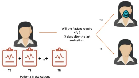
3.2 Workflow of the methodology for ALS prognostic prediction using patient snapshots 28 3.3 Problem Formulation: Given a set of N consecutive patient evaluations, can we predict the need for Non-Invasive Ventilation (NIV) k days after the last evaluation? 36 3.4 Example of learning examples using multiple snapshots. . . 36
3.5 Example of transformation using temporal aggregation. . . 38
4.2 Problem Reformulation using Progression Groups: Knowing the Patient current state, as well as their progression group can we predict the need for Non-Invasive Ventilation k days after, using group specific models? . . . 47
4.3 Workflow of the proposed methodology for ALS prognostic prediction using patient snapshots and progression groups. . . 48
4.4 Problem Reformulation using Progression Groups: Knowing the Patient clinical history (follow-up), as well as their progression group can we predict the need for Non-Invasive Ventilation within k days from the last evaluation, using specialized models for each group? . . . 57
5.1 Problem reformulation using Patient Profiles: Knowing the Patient current state, as well as the attributed patient profile (for a given clinical profile) can we predict the need for NIV within a given time window? . . . 66
5.2 Workflow of the proposed methodology for ALS prognostic prediction using patient snapshots and patient profiles. . . 67
2.1 Confusion Matrix. . . 16
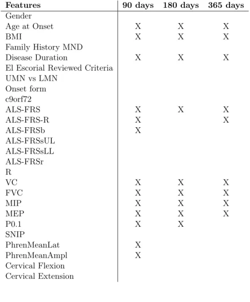
2.2 Available Features in the ALS dataset. . . 25
3.1 Statistics and Class distribution for time windows of k=90,180,365 days. . . 29
3.2 Parameters and correspondent ranges tested for each classifier. . . 30
3.3 Selected Features by the Feature Selection Ensemble for each time window. . . . 30
3.4 Proportion of Missing Data before and after Last Observation Carried Forward (LOCF) imputation. . . 32
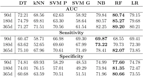
3.5 AUC, Sensitivity and Specificity results for the prognostic models for 90, 180 and 365 days. . . 32
3.6 AUC, Sensitivity and Specificity results for the prognostic models for the 90, 180 and 365 days Time Windows using Feature Selection. . . 34
3.7 AUC, Sensitivity, and Specificity results for the prognostic models for the 90, 180 and 365 days Time Windows using Missing Value Imputation. . . 34
3.8 Best results achieved for baseline models using the patients current condition. . . 35
3.9 Statistics and Class distribution for time windows of k=90,180, and 365 days. . . 37
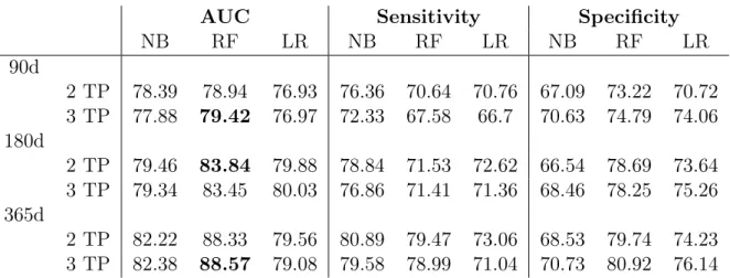
3.10 AUC, Sensitivity and Specificity results for the prognostic models using 2 and 3 time points (TP) for each time windows of k=90,180,365 days. . . 39
3.11 AUC, Sensitivity and Specificity results for the prognostic models using 2 or 3 patient time points (TP) using Feature Selection . . . 40
3.12 AUC, Sensitivity and Specificity results for the prognostic models using 2 or 3 time points (TP) for the 90, 180 and 365 days Time Windows using Missing Value Imputation. . . 41
3.13 AUC, Sensitivity and Specificity results for the prognostic models using temporal aggregation. . . 42
3.14 Best results obtained for the baseline models using 1 TP (current condition) as well as using 2 and 3 TP (clinical history). . . 43
4.1 Statistics and Class distribution for time windows of k=90,180, and 365, for each progression group. . . 47
4.2 Selected Features for each progression groups and each time window. . . 50
4.3 AUC, Sensitivity and Specificity results for the prognostic models for the 90, 180 and 365 days Time Windows, as well as for each Progression Group. . . 51
4.4 AUC, Sensitivity and Specificity results for the prognostic models for the 90, 180 and 365 days Time Windows, as well as for each Progression Group using Feature Selection. . . 53
4.5 AUC, Sensitivity and Specificity results for the prognostic models for the 90, 180 and 365 days Time Windows, as well as for each Progression Group using Missing Value Imputation. . . 54
4.6 AUC, Sensitivity and Specificity results for the prognostic models built without progression groups (baseline models) for the 90, 180 and 365 days Time Windows, relative to each Progression Group . . . 55
4.7 Best results obtained for the specialized models for each progression group, using the patients current condition. . . 56
4.8 Statistics and Class distribution for time windows of k=90,180, and 365, for each progression group using 2 and 3 time points TP. . . 58
4.9 AUC, Sensitivity and Specificity results for the prognostic models for the 90, 180 and 365 days Time Windows, as well as for each Progression Group using 2 and 3 Time Points. . . 59
4.10 AUC, Sensitivity and Specificity results for the prognostic models for the 90, 180 and 365 days Time Windows, as well as for each Progression Group, using 2 Time Points (TP). . . 60
4.11 AUC, Sensitivity and Specificity results for the prognostic models for the 90, 180 and 365 days Time Windows, as well as for each Progression Group, using 3 Time Points (TP). . . 61
4.12 Best results obtained for the specialized models for each disease progression group using 1 TP (current condition) as well as using 2 and 3 TP (clinical history). . . 63
5.1 Statistics and class distribution for each profile, across all time windows. . . 69
5.2 Selected features by the Feature Selection Ensemble (FSE) for each clinical profile and respective set of Patient Profiles. . . 70
5.3 AUC, Sensitivity and Specificity results for the prognostic models for the 90, 180 and 365 days Time Windows, as well as for each Clinical Profile and respective set of Patient Profiles. . . 71
5.4 AUC, Sensitivity and Specificity results for the prognostic models using Feature Selection for the 90, 180 and 365 days Time Windows, as well as for each Clinical Profile and respective set Patient Profiles. . . 72
5.5 AUC, Sensitivity and Specificity results for the prognostic models using Misssing Value Imputation for the 90, 180 and 365 days Time Windows, as well as for each Clinical Profile and respective set Patient Profiles. . . 73
Introduction
1.1 Motivation
Amyotrophic Lateral Sclerosis (ALS) is a neurodegenerative disease characterized by the pro-gressive loss of motor neurons in the brain and spinal cord, which leads to muscular weakness and ultimately ends in death (van Es et al.(2017)). The life expectancy of an ALS patient is 3 to 5 years after disease onset (Brown & Al-Chalabi (2017)). There is no cure or known causes for ALS, and the heterogeneity of the disease makes it difficult to understand its underlying mechanisms. Thus finding solutions to cure or slow disease progression is a challenge. Therefore, efforts must be taken to find solutions that can improve patient’s prognosis and help to maintain the patients quality of life.
ALS studies focus mainly on patient survival (Georgoulopoulou et al., 2013; Pastula et al.,
2009;Traynor et al.,2003), exploring the impact of diagnostic delay (Gupta et al.(2012)), un-derstanding and defining ALS sub-types (Chiò et al.(2011)), or finding relevant clinical features that can be used both as diagnostic or as prognostic predictors (Creemers et al.(2015)).
With the rapid advance in the fields of computer science, genetics, imaging, and other tech-nologies came the promise of a new form of medicine, so-called precision medicine. It can be defined as targeted treatments for individual patients based on their genetic, phenotypic or psy-chological characteristics (Larry Jameson & Longo(2015)). Although this approach has already shown promising results in areas such as cancer, it is only now beginning to be used in ALS studies (Zou et al.(2016)).
In recent years there has been increasing attention to patient stratification in ALS. By group-ing patients either by their progression level (Westeneng et al. (2018)) or by a set of prognostic features (Ganesalingam et al.(2009)), it has been shown to be possible to design new treatments
or disease management strategies which are specialized for a specific group of patients that has something in common.
Since respiratory failure is responsible for the majority of deaths in ALS patients, there is a need to prevent the decline in respiratory capacity as earlier as possible. Non-invasive ventilation (NIV) is the standard treatment for respiratory impairment in ALS patients and has proven to prolong survival and improve quality of life, especially when administered in earlier stages (Georges et al.(2014)).
1.2 Problem Formulation and Original Contributions
This dissertation is the follow-up to the work developed in André Carreiro’s PhD Thesis (Carreiro
(2016)) in which he proposes an integrative approach combining supervised learning, clinical data of ALS patients and the insights from ALS experts, to develop prognostic models to predict changes in the clinical state of patients according to a given time window.
In this dissertation we will revisit and explore further some of the addressed questions, using an updated dataset containing more data and some approach alterations. Those questions being revisited are:
• Given a patient evaluation, can we predict if a given patient will require NIV within a certain time window?
• Given a set of consecutive patient evaluations (T1, T2,..., Tk) can we predict if the patient will require NIV within a certain time window after evaluation Tk?
The dataset used to answer the questions above is the Portuguese ALS dataset presented in Section 2.5. Furthermore, to the questions above (also tackeld by Carreiro et al), and whose results obtained with the updated data we use as baseline, we propose two different approaches to stratify patients: according to disease progression and patient profiles (Sections 2.4.1 and 2.4.2). We also investigate whether using these groups in specialized models for each group yields better results when answering the questions above.
Part of the contribution in this thesis we presented at The Sixth Workshop on Data Mining in Biomedical Informatics and Healthcare, held in conjunction with the IEEE International Conference on Data Mining (ICDM’18). The publication is presented in Appendix A.
1.3 Thesis Outline
Other than the current, this thesis is outlined over 5 additional chapters:
• Chapter 2 presents the background regarding ALS, Patient Stratification, Prognostic Pre-diction as well as concepts of Machine Learning and Data Mining techniques used in this dissertation. It also provides an overview of the dataset used in this work;
• Chapter 3 tackles the two questions proposed above, and presents the baseline results for this dissertation;
• Chapter 4 explores the first approach to patient stratification, presenting the results of the prognostic models using disease progression groups;
• Chapter 5 explores the second approach to patient stratification, presenting the results of the prognostic models using patient profiles;
Background
2.1 Amyotrophic Lateral Sclerosis
Amyotrophic lateral sclerosis (ALS), also known as Motor Neuron Disease (MND) is a complex neurodegenerative disease characterized by the progressive loss of motor neurons in the brain and spinal cord (van Es et al.(2017)).
The prevalence of the disease is approximately 3-5 cases per 100.000 individuals. Although this is a seemingly low number for the general population, the risk of developing ALS increases in the latter years of life, reaching a risk of 1:300 at the age of 85 (Martin et al.(2017)).
Around 10% of ALS cases are familial (patients which have/had relatives with ALS) and the remaining 90% are considered sporadic. Although there are no major differences in the presentation and progression, familial ALS patients present an earlier disease onset than the ones with sporadic ALS (Brown & Al-Chalabi (2017)). The disease onset is within 58-63 years for sporadic ALS, and within 43-63 years for familial ALS (Andersen et al.(2012)).
With recent advances in genetics, more information about the disease is being discovered, providing new insights into what causes ALS and what are the risk factors. More than 20 genes related to ALS have been discovered in recent years, three of them seem to be more relevant than the others (Martin et al. (2017)). The SOD1 gene was the first gene identified as being associated with ALS and for a long time the only gene known to be related with this disease (van Es et al. (2017)). SOD1 mutations are present in approximately 20% of familial ALS patients and 5% of sporadic ALS patients. The second gene, TARDBP, represents approximately 5-10% of familial ALS mutations (Zarei et al. (2015)). The last gene, C9orf72, is responsible for 30% of familial ALS and up to 10% of sporadic ALS, being the gene with the biggest association to ALS (Martin et al.(2017)). Around 50-60% of the familial ALS patients have mutations in the described genes. However, there are still 40-50% (Zarei et al.(2015)) of the familial ALS cases
that are not linked to any gene, and an even greater percentage regarding sporadic ALS cases. The Mine project (Mine & Sequencing(2018)) launched a large-scale whole-genome sequencing study using 15 000 ALS patients and 7500 controls. The aim of this project is to discover new genetic risk factors and further elucidating the genetic basis of ALS. The ONWebDUALS project (ONtology-based Web Database for Understanding Amyotrophic Lateral Sclerosis) aims to create a standardized European database, with genetic and phenotypic information of ALS patients, in order to identify relevant risk and prognostic factors in ALS.
Non-genetic factors have also been linked to ALS, such as exposure to toxins, smoking, exces-sive physical activity, occupation, dietary factors and changes in immunity, especially regarding sporadic ALS patients (Zou et al.(2016)).
The initial symptoms of the disease are muscle weakness, twitching, and cramping, which can later lead to muscle impairment. These usually start in the limbs. However, a third of the ALS patients have a bulbar onset, characterized by difficulty in swallowing, chewing, and speaking (Brown & Al-Chalabi(2017)). Dyspnea and dysphagia are usually developed in more advanced stages of the disease (Zarei et al. (2015)). The eye and bladder muscles are usually the less affected, showing signs of impairment only in the latest stages of the disease (Brown & Al-Chalabi (2017)).
Regarding diagnosis, there is usually a delay of 13–18 months from the onset of a patient’s symptoms to confirmation of the diagnosis (Zarei et al. (2015)). This can be a consequence of the low prevalence of the disease, meaning it is not common for a primary care physician to have many patients with ALS. Moreover, the overlap with other neurodegenerative diseases may difficult and delay the diagnosis (Hardiman et al.(2011)). These delays can worsen the prognosis of the patients since therapies have usually better outcomes when applied in the early stages of the disease. There is not yet a single test to directly diagnose ALS. Therefore, the initial steps towards diagnosis are the exclusion of other neurodegenerative diseases as well as other limb dysfunction causers. Then, Electrodiagnostic tests, neuroimaging, or laboratory tests can be used to find a final diagnosis(Zarei et al.(2015)).
There is no definitive cure for ALS. Thus, available treatments are focused on slowing the disease rather than stopping it. Riluzole is the only approved drug treatment, showing an increase in survival up to 14.8 months (van Es et al.(2017)). Other available treatments consist in symptom relief and progression. Symptomatic intervention and supporting care for ALS patients include the provision of ventilatory support, nasogastric feeding, and prevention of aspiration (Brown & Al-Chalabi (2017)). The latter consists in control of salivary secretions and use of cough-assist devices. Moreover, Nasogastric feeding helps preventing malnutrition, common in ALS patients, which improves survival and quality of life (van Es et al. (2017).
The majority of ALS patients usually die of respiratory failure within 3-5 years from disease onset (Brown & Al-Chalabi(2017)). Thus, preventive treatments to maintain respiratory muscle function are vital for these patients. Non-Invasive Ventilation (NIV) is the only treatment to prevent respiratory failure in ALS patients (Georges et al. (2014)). The use of NIV, when administrated in earlier stages of the disease, has shown to improve survival in ALS patients and their quality of life.
With no definitive cure available, the focus in ALS patients’ care is to slow disease progression, improve prognosis, and maintain the quality of life. To achieve these objectives, a multidisci-plinary team of clinicians, together with the caregivers, is imperative to ensure the patient has the best care, resulting in increasing survival (Brown & Al-Chalabi(2017)). In this context, dur-ing clinical follow-up, the patient’s condition is evaluated usdur-ing ALS related functional scores, Respiratory and Neurophysiological tests, as well as other physical values. These Longitudinal data together with the static data collected at disease diagnosis is used for prognostic prediction.
2.2 Data Mining Techniques
Data Mining is a multidisciplinary subject that combines domains such as statistics, machine learning, pattern recognition, database and data warehouse systems, information retrieval, visu-alization, algorithms and high-performance computing (Han et al.(2012)). Its main purpose is to extract new and useful information from collections of data (Laxman & Sastry(2006)). Data Mining techniques allow us to find patterns and relationships in data which could go unnoticed to the human eye (Sharma et al. (2018)). It has applications in many fields such as science, marketing, finance, healthcare or retail (Fayyad et al.(1996)).
2.2.1 Data Preprocessing 2.2.1.1 Feature Selection
It is common in Machine Learning (ML) problems, to have a dataset that has a very high number of features (dimensions). With high dimensionality, the amount of data needed to build reliable models is also very high. Without enough learning instances the performance of the classifiers can be hindered (Bolón-Canedo et al.(2014)).
Having too many features can be detrimental for the model’s performance, and this is a known problem, commonly called by "The curse of dimensionality" (Somorjai et al. (2003)). Dimensionality Reduction is one of the most popular techniques to deal with this issue. It can be divided into Feature Extraction and Feature selection. Feature extraction combines the original features into a new set of feature with reduced dimensionality (Tang et al. (2014)). As
for Feature Selection (FS), it selects a subset of features which better describe the data and reduce the effects of noisy and irrelevant features (Chandrashekar & Sahin(2014)).
Using FS to downsize the number of features in a dataset, can bring several benefits: data visualization becomes easier due to the lower dimensionality, reduces storage requirements as well as reduced training and utilization times (Guyon & Elisseeff(2003)).
For a recent survey on FS see (Li et al.(2017)). In this survey the authors divide the methods in filter, wrapper, and embedded methods.
2.2.1.2 Missing Value Imputation
Missing data is common in almost all real datasets. However, missing data means lack of infor-mation, which can be problematic as some data mining methods rely on complete datasets to work.
There are 3 types of missing data: missing completely at random (MCAR), missing at random (MAR) and missing not at random (MNAR) (Newgard & Lewis (2015)). MCAR is the least common and also the least problematic since it yields less biased results. MAR is a more realistic version on MCAR, but can lead to biased results. Lastly, MNAR is the most problematic of the three, making almost impossible to find a statistically approach to deal with this type.
There are mainly two ways to deal with missing data: deletion and imputation (Cheema
(2014)). Deletion methods consist in removing either instances or columns with missing values. However, in datasets with low quantities of data or with many missing data this can lead to a considerable loss of information. On the other hand, imputation methods do not remove any instances or columns, but rather replace the missing values with predicted values obtained from the study of the whole dataset.
Missing Value Imputation (MVI) methods can be divided into two groups: Single Imputa-tion (SI) or Multiple ImputaImputa-tion (MI). Single imputaImputa-tion methods replace the missing value with plausible values by observing the characteristics of the population. The most common method is Mean Imputation which imputes missing values using the population mean for the variable. However, when performed in datasets with large quantities of missing data, it leads to a loss of feature variance and correlation distortion that can lead to a biased dataset (Josse & Husson
(2012)). Last Observation Carried Forward (LOCF) presents as an alternative to Mean Impu-tation, by assuming that the value does not change from the last observation (Newgard & Lewis
(2015)). This methodology is especially common in clinical datasets, where longitudinal data is available.
MI methods consist in imputing multiple versions of the same dataset, each with a different imputation methodology (Donders et al. (2006)).
2.2.1.3 Dealing with Imbalanced Data
Having an imbalanced data, means having a dataset where there are more instances for one of the class values than the other. In imbalanced data the number of available instances for each of the classes to be learned is not the same.
Dealing with imbalanced datasets presents a challenge for some machine learning problems, as most machine learning algorithms assume that classes are balanced. However, in real-life problems, this is seldom the case (Krawczyk(2016)).
Undersampling and Oversampling are two opposite alternatives to deal with class imbalance. The first consists in removing instances from the majority class and the latter on adding instances for the minority class, both of them ensuring a balanced dataset (Rahman & Davis (2013)). In undersampling techniques, instances of the majority class are randomly removed until the number of instances for each class is equalized. Problems with this method lie in the possible loss of information from the removed instances and the resulting low number of overall instances when the minority class has only a few instances (He & Garcia(2009)). Oversampling techniques overcome these problems by keeping all instances and resampling minority class instances until class balance is achieved. This can be done by simply resampling the minority instances, however, this easily can lead to a biased dataset (He & Garcia(2009)).
Synthetic Minority Over-sampling Technique (SMOTE) proposes an oversampling alterna-tive, as it creates synthetic learning instances for the minority class by using k-Nearest Neighbors method to find similar k instances to one of the minority class examples, ans use them to create a new instance (Chawla et al. (2002)).
2.2.2 Machine Learning 2.2.2.1 Supervised Learning
Supervised Learning algorithms consist in learning a function from a set of training data able to predict the desired output. Each training instance consists of a vector with information on each variable in the data, and a truth value for the outcome we are trying to predict (lable/class). After training, the model should be able to receive the feature vector as input, and according to the function learned by the model, output a prediction for the outcome.
These algorithms can be divided into two groups: classification and regression. The first outputs the prediction in a discrete value, usually binary, and the latter outputs a continuous value for the prediction.
Decision Trees
Decision Tree (DT) is a simple and powerful statistical tool that can be used in classification, prediction or even data manipulation (Song & Lu (2015)). The features are represented as internal nodes of the tree, and each one of its resulting branches are possible values (discrete) or ranges (continuous) of each feature. The final nodes, or leaves, are the predictions (Han et al.
(2012)). In Figure2.1 we show a DT example used to predict if a customer will or will not buy a computer.
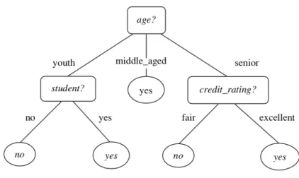
Figure 2.1: Example of a Decision Tree for the following problem: "Will the customer buy or not buy a computer?". Rectangle boxes are the attributes, branches are the possible values and oval boxes the predictions. Adapted from Han et al.(2012)
The top of the DT is the feature which better separates data, according to the class values of each instance. The next internal node for each branch will be the best describing feature for the data subset that follows each branch. This last step is repeated until either all features have been used, or all the final branches lead to a prediction. When we reach at a feature in which each value leads to a single prediction, then there is no need to look further in the remaining features and the branches of that feature will lead to the leaves (final predictions) of the tree. In situations where even with all available features, there is no combination that allows reaching single predictions, we have to resort to majority voting. This consists in choosing the prediction value for each branch according to the most popular value (Hu et al.(2012)).
The simplicity allied with easy understanding, interpretation, and visualization are some of the advantages of using this algorithm (Song & Lu (2015)). However, for datasets with high dimensionality, visualization and interpretation may be challenging when using DT.
Random Forests
Random Forests (RF) is an ensemble learning method that combines several Decision Trees to make a prediction. Each DT is trained with a random subset of features available.
This method has shown improvement in classification problems as the final prediction is de-cided by the majority vote of each singular tree prediction (Breiman(2001)).
K-Nearest Neighbors
The k-Nearest Neighbor (kNN) algorithm is a commonly used classifier among many classifi-cation problems, in which the output is computed by accessing the outcomes for a given number of learning instances (k) closer to the input instance. It is considered a lazy learner since the classifier is not really trained before its use, but rather trained at the moment of use (Han et al.
(2012)).
When a new instance is fed to the classifier, the algorithm finds its k-nearest instances. The most common metric to compute the distances between instances is the Euclidean distance, however, other distances can be used (Liu et al. (2004)). In order to classify the new instance, the classifier looks at to the outcome of each neighbor and choses according to the majority class of the neighbors. When using kNN, it is advised to use an odd number of neighbors to prevent ties in classification. However, one solution to solve the tie would be using the majority class of the entire dataset or the class of the nearest neighbor. Moreover, to avoid overfitting its advised against using a larger k.
An example of the described algorithm can be seen in Figure2.2
Figure 2.2: Example of a k-Nearest Neighbor classifier using 3 neighbors (k=3). The blue rectangles are instances for one class and green circles instances for the other. The orange triangle is the new instance.
Support Vector Machines (SVM) are powerful models commonly used in nonlinear classifica-tion, regression and outliers detection (Aha et al.(1991)).
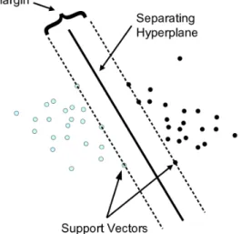
In this algorithm, data is mapped in a multidimensional space (one dimension per feature). Then, the SVM tries to find linear hyperplanes that separate the classes with maximal margins, called support vectors (Hsu et al.(2008)). Figure2.3shows an example of how support vectors are created. When linear separation is not possible, SVM uses the kernel technique to automatically release non-linear mappings in the feature space (Furey et al.(2000)). The most common kernels used are linear, polynomial, radial basis function (RBF), and sigmoid. All support vectors computed are then combined into a function that receives a feature vector as input and outputs a prediction for the outcome in the study.
Figure 2.3: Example of a SVM. Figure adapted fromAha et al. (1991).
Although SVMs are very robust, they usually work best for problems with fewer features, since a higher number of features translates to a higher number of dimensions and a higher number of support vectors to be computed, which can be detrimental to the performance of the classifier. To use SVM in high dimensional problems it is advised to build the classifiers with only a subset of the features (Hsu et al. (2008)).
Naive Bayes
The Naive Bayes (NB) classifier is a simple, probabilistic and easy to use algorithm that has been showing promising results in several applications. It is called Naive because it is based on the assumption that the features are independent of the class (Rish (2001)).
Let C = (c1, ..., ck) be the class variable we are trying to predict and let X be a vector
the classifier predicts its class according to the highest posterior probabilities that are conditioned on X (Han et al. (2012)). The posterior probability for each value i = 1, ..., k is obtained by:
p(C = ci|X = x) =
p(C = ci)p(X = x|C = ci)
p(X = x) . (2.1)
As NB follows the assumption that all variables are independent, then,2.1can also be defined by the sum the conditional probabilities of each variable, according to a class value:
p(X|C = ci) =
Y
n
p(X = xj|C = ci). (2.2)
Another assumption followed by the NB classifier is that all numeric attributes follow a Gaussian/Normal distribution. Thus there is a need to estimate a set of parameters from the training data (mean and standard deviation). Density estimation methods have explored ways to overcome the problems with this last assumption. These methods work by averaging over a set of Gaussian kernels:
p(X|C = ci) = 1 n X i G(X, µ, ), (2.3)
where i ranges each training point in class ci, µ = xi and = p1ni , where ni is the number of
instances with class value c1.
Logistic Regression
Regression methods are popular in data analysis due to their capability to describe relation-ships between the target variable and one or more explanatory variables. When using a discrete target, Logistic Regression (LR) is the standard method used (Hosmer & Lemeshow(2000)) and is based on the following logistic function:
f (z) = e
z
ez+ 1 = (1 + e
z) 1. (2.4)
One of the advantages of using LR is that the classifier outputs a real predicted value for each class value, between 0 and 1, that allows to look not only to the prediction but also to its probability (Naive Bayes also does that). The input of the classifier z, usually called logit, is a representation of the explanatory variables of the problem and can be defined as:
where i is the regression coefficient for the variable xi and 0 is the probability of the outcome
if all variables do not contribute to the problem.
The threshold to determine the predicted class is usually 0.5 in binary classes, meaning that if the probability for a given class value is superior to 0.5 the makes the prediction for that value, and if the probability is lower than 0.5, the classifier prediction is made for the other value. 2.2.2.2 Unsupervised Learning
As opposed to Supervised Learning, Unsupervised Learning methods learn from unlabeled data to find functions that describe it. These methods are usually used to find groups and stratify data and to find hidden patterns. Clustering, Anomaly Detection, Neural Networks and latent variable models are some of the different fields.
Clustering is one of the most popular fields, in which the algorithms partition the data in subsets (clusters) according to the similarities and dissimilarities between instances. The clusters created can be helpful to retrieve new information from the similarity in each cluster but also from the differences between the clusters.
k-Means
K-Means is the simplest and most popular among all clustering algorithms. In this method the number of clusters (k) is defined apriori (Krishna & Murty (1999)).
In order to create the clusters, k random instances of data are chosen to be the initial centroids (points in the middle of each cluster). Then, the remaining instances are individually compared to each of the centroids and assigned to the cluster of the closest one.
After the first iteration, new centroids are computed using the mean of all instances inside one cluster. Then, all instances are once more compared to each centroid and assigned to the closest centroid. This process repeats until the point of conversion (when there is no change in the composition of the centroids between iterations) or until they reach the maximum number of iterations.
Although being simple and presenting overall acceptable results, there are some disadvantages to this method. One, is the need to have prior knowledge of the number of groups to be created. Another disadvantage lies in the number of iterations that change with the number of instances, the number of clusters, and the complexity of the problem, which can make computationally expensive (Alsabti et al.(1997)).
Hierarchical Clustering
Hierarchical Clustering (HC) methods create clusters according to a hierarchy and can be divided in two groups: divisive and agglomerative, the latter being the most popular.
Agglomerative Hierarchical Clustering (AHC) methods, work by interactively combining the two closest objects or clusters until all data falls in the same cluster. An opposite approach is used when using the divisive methods.
In the first step of the AHC process, the number of clusters is equal to the number of instances. Then, a proximity matrix is computed to register the distances between each two points of data. The two closest points are then combined in the same cluster and the proximity matrix is recalculated swapping the two instances for the cluster centroid and computing its distance to each of the left over instances. This process repeats itself until achieving one cluster with all instances in it.
When dealing with a relative low number of instances, the results of the AHC can be shown by a dendogram, which provides an easy visualization (see Figure 2.4). A different number of clusters can be derived by choosing different cut-off in the similarity value.
Figure 2.4: Example of a Agglomerative Hierarchical Clustering.
2.2.2.3 Model Evaluation and Selection Cross-Validation
Cross-Validation (CV) is a popular method for model selection and parameter estimation in supervised learning. It works by splitting data a number of times, in order estimate the performance of each classifier. A subset of data, called training set, is used to train the classifiers, while the rest, testing set, is then used to assess its performance (Arlot & Celisse(2009)).
There are many ways of splitting the data, but the most popular are: Leave-one-out (LOO), Leave-p-out (LPO) and K-Fold (VF). The first two approaches are considered exhaustive splitters and the latter a partial splitter. In LOO, each instance is successively remove from the sample
and used for model validation, as for LPO, each possible subset of p instances is left out for validation.
In k-Fold CV data is partitioned in k subsets. In each iteration one subset (fold) is held out for test, while the other subsets are used for training purposes (Arlot & Celisse (2009)). This method is much less time consuming in comparison with the other methods as the number of iterations is much lower (one iteration for each fold). However, when splitting data in folds, the folds created can be very similar to each other. To overcome this problem, v-Fold CV is usually performed multiple times, each time generating different folds.
Performance Metrics for Supervised Learning
Confusion Matrix
A confusion matrix is a matrix of c x c dimensions, where c is the number of classes, usually used to compute performance metrics for model evaluation. The rows usually represent the predicted values and the columns the real values of the class. In binary classification we have a 2 x2 table, as shown in the example in Table2.1.
Table 2.1: Confusion Matrix. Predicted Class True Class TC1 PC1TP PC2FN
TC2 FP TN
These tables allow us to evaluate where the classifiers are performing correct or wrong predic-tions. We can see this by the four indicators provided: Number of True Positives, True Negatives, False Positives and False Negatives, where:
• True Positive (TP): an instance from the positive class that is classified as positive; • False Negative (FN): an instance from the positive class that is classified as negative; • True Negative (TN): an instance from the negative class that is classified as negative; • False Positive (FP): an instance from the negative class that is classified as positive.
Accuracy
Accuracy gives us the information about how many instances were correctly classified:
Accuracy = T P + T N
T P + F P + T N + F N. (2.6)
However, when dealing with imbalanced classes, this metric can be biased by how the classi-fier performs in classifying the majority class.
Sensitivity
Sensitivity, also known as recall or true positive rate, shows the proportion of positive in-stances that were classified as such:
Sensitivity = T P
T P + F N. (2.7)
Specificity
Specificity, selectivity or true negative rate shows the same information as the sensitivity metric, but for the negative class. Thus, it gives information about the proportion of negative instances that were correctly classified:
Specif icity = T N
T N + F P (2.8)
ROC and AUC
When evaluating a classifier using the metrics described above, we have to be careful and take into account the proportions of each class value as to not be biased by the results.
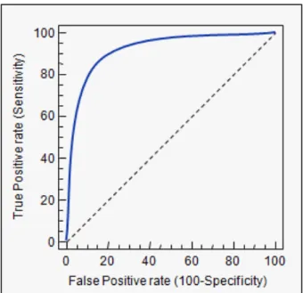
The receiver operating characteristic (ROC) curve combines the Sensitivity and Specificity metrics in a graph for each classification threshold. This results in a graph that shows the performance of a classification model. Figure 2.5shows an example of a ROC curve.
The closer the curve is to the upper left corner the better the performance of the classifier, since the sensitivity and specificity measures are maximized.
The ROC is also used to compute one of the most popular metrics in performance evaluation, the Area Under the ROC Curve, also known as AUC. As it says in the name, this metric measures the area under the ROC curve. The AUC metric can be defined as either the a representation
Figure 2.5: Example of a ROC curve.
of the classifier ability to separate the classes or the probability of an instance with a given class value being classified as such.
Cluster Validation
Determining the best number of clusters in a dataset is a common problem in when using clustering, especially when using k-means, where we need to tell the model how many cluster we want to create. There are some measures and scores that can be used to determine the optimal number of clusters to create for our data.
Silhouette Score
The Silhouette score for a given instance in our dataset gives us information on how close our instance is to the other instances in the same cluster. This score can vary between -1 and 1. Scores close to 1 mean the instance is in the right cluster, while scores close to -1 mean the instance is in the wrong cluster.
To determine the optimal number of clusters in a dataset, we can run the clustering algorithms with different number of clusters, and use the average Silhouette score to evaluate how good are the clusters. The clustering with higher Silhouette score, is the one with optimal number of clusters.
2.3 Prognostic Prediction in ALS
As stated previously, with no definitive cure for ALS, efforts are then focused on designing treatments that improve the prognosis of patients and their quality of life. However, many treatments are more effective when administered earlier on. Prognostic prediction can be a key tool in this context. By predicting a given prognosis beforehand, clinicians are then able to administer appropriate treatment before being to late. Nevertheless, the number of studies regarding prognostic prediction in ALS are scarce. Current studies usually focus in finding prognostic biomarkers associated with patient survival (Polkey et al.,2017;Sato et al.,2015).
In the work prior to this dissertation, André Carreiro (Carreiro(2016))proposed an approach to predict the need of NIV in patients with ALS. He advanced the state of the arr by, rather than predicting the immediate need, proposing the use of time windows. This allows to answer the following question: "Given a patient’s current condition, will the patient need NIV within k days?". Longitudinal Data from a cohort of 758 patients from the ALS clinic of the Translational Clinical Physiology Unit, Hospital de Santa Maria, Lisbon was used to build the prognostic models.
To obtain learning instances comprising all information about a patient’s condition and the need for NIV some prepossessing steps had to be taken. The first was to transform the demo-graphic data and information of each clinical test into Patient Snapshots. Then, as the snapshot only accounts for the current condition, an Evolution Class (E) was created, to label each in-stance with the information about the patient’s needed for NIV within a given time window. These prepossessing steps are detailed in Section 2.3.1. After, several classifiers were trained to predict this outcome. The results obtained were promising and helped to prove that prognostic prediction models can be useful tool in helping clinicians in their decision making process.
The DREAM-Phil Bowen ALS Prediction Prize4Life Challenge (Küffner et al. (2015)) en-couraged researchers to use clinical trial data to predict disease progression in 3 to 12 months. In fact knowing how patients progress can be useful when designing clinical trials and help clini-cians in better determining their patients prognosis. This led to several proposals being presented that helped validating various prognostic features described in the literature (Westeneng et al.
(2018)).
2.3.1 Patient Snapshots and Evolution Class
In order for a classifier to be trained, it needs labeled learning instances. These instances are composed by a feature vector, which has the information about a patients current condition and
a class value, which has the information about the outcome on which the classifier will be trained to predict.
The original data used in André Carreiro’s work (Carreiro (2016)) was composed of de-mographic data about the patient, as well as a set of prescribed tests that are usually done periodically at each appointment. However, since many times the patient cannot perform all tests in the same day, but rather do it in a span of a few days or weeks, it becomes difficult to align all tests together to generate a snapshot that resembles that period. An approach to solve this problem is grouping the tests by their date. A good methodology to achieve this is using an Agglomerative Hierarchical Clustering scheme. This approach was also proposed by André Carreiro as an alternative to the standard approach based on pivot tables, which results in a greater number of instances, but with a higher proportion of missing values.
To build patient snapshots from the original data, the Hierarchical Clustering algorithm will group all the patient’s tests by date so that the tests performed at closer dates will end at the same group, thus creating a snapshot. However, there are some restrictions to the algorithm in order to have cohesive snapshots. First, two observations of the same test cannot be in the same group, and second, all observations in a group must have the same NIV status, meaning that there cannot be groups that have tests performed when the NIV status is 0 (the patient does not require NIV at current time) and tests where NIV status is 1 (the patient requires NIV at current time). The result from this approach is a dataset where each row is a patient observation, also called a patient snapshot, where each feature is the result from each test performed, and a NIV status class, with the information about the need or not for NIV at the time of said evaluation. A fictional example of the described process is illustrated in Figure 2.6.
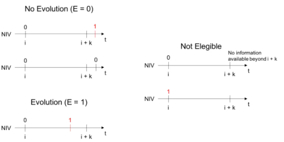
After this step, what we have is the information on the patient’s current condition and the current need or not need for NIV. However, since the goal is to predict the need for NIV beforehand, there is one more preprocessing step needed. Therefore, an Evolution class (E) is added in order to accommodate the temporal information regarding the NIV status. Essentially, if a patient needs NIV within a time window of k days from the current evaluation, then E=1 (the patient evolves to need NIV). If within the same k days, the patient does not need NIV, then E=0 (The patient does not evolve to need NIV).
The creation of this class has also some restrictions. They are as follows:
• Snapshots from patients who already require NIV at the first evaluation cannot be used as learning instances;
• Snapshots where there is no information about the NIV status of the patient after the time window used cannot be used as learning instances.
Figure2.7illustrates the possible cases for the creation of the Evolution class (E). Moreover, an illustration of this last preprocessing step is presented in Figure 2.8.
Figure 2.7: Definition of the Evolution Class (E) according to the patient’s requirement of NIV in the interval of k days. i is the median date of the snapshot. E=1 means the patient requires NIV and E=0 means the patient does not require NIV. Adapted fromCarreiro(2016).
2.4 Patient Stratification in ALS
Due to ALS heterogeneous nature, special attention has been given in recent years to patient stratification. The idea is that designing specialized models using groups of patients stratified according to their progression (Westeneng et al.(2018)), or specific sets of prognostic biomarkers
Figure 2.8: Example of creating learning instances using a time window of 90 days.
(Ganesalingam et al.(2009)) may help understand the underlying mechanisms of the disease and provide a new perspective on how to plan clinical trials and better manage disease progression.
In this dissertation, we propose two approaches to perform patient stratification in ALS patients: 1) disease progression groups and 2) patient profiles. The two methodologies are further explained in Sections 2.4.1 and 2.4.2.
2.4.1 Disease Progression Groups
Although the average survival of an ALS patient is about 3-5 years, survival can vary between less than a year to over 10 years (Martin et al. (2017)). This shows that disease progression is not equal in all patients, thus making hindering to have treatments that perform well for all patients.
One way to analyze disease progression is by considering at the ALS Functional Rating Scale (ALSFRS) (Proudfoot et al. (2016)) decay in a period of time. The ALSFRS is a standard test used by physicians in practice that can be used to estimate the outcome of a treatment or the progression of the disease. Although very popular, this scale has only a small respiratory com-ponent. Given that respiratory failure is the most common cause of death in ALS patients, the ALS functional rating scale-revised (ALSFRS-R) was later proposed (Cedarbaum et al. (1999)). This new scale adds additional respiratory assessments and quickly became the preferred test to
quantify disease progression (Simon et al.(2014)). The test is composed of 13 questions, where each should be answered using a 5-point scale, ranging from 0 to 4, where 0 corresponds the worse condition and 4 is the best. The questions addressed by this scale are: 1) Speech, 2) salivation, 3) swallowing, 4) handwriting, 5) cutting and handling utensils, 6) dressing and hygiene, 7)turning in bed and adjusting bed clothes, 8) walking, 9) climbing stairs, 10) breathing, 11) dyspnea, 12) orthopnea, and 13) the need of respiratory support (Castrillo-Viguera et al. (2010)).
By measuring the change in ALSFRS-R over time, we can estimate how is the disease pro-gressing and infer about the survival of the patient (Kimura et al. (2006)). By using the infor-mation about the time of first symptoms and the time of the first appointment we can compute its progression rate using the following equation:
P rogressionRate = 48 ALSF RSR1stV isit t1stSymptoms;1stV isit
, (2.9)
where 48 is the maximum score of the ALSFRS-R scale (and the assumed score of a patient at the time of its first symptoms), ALSF RSR1stV isitis the ALSFRS-R score of a given patient
at the beginning of the first appointment (diagnosis) and t1stSymptoms;1stV isit is the time in
months between the time of first symptoms and the first visit.
By knowing each patient’s progression rate we can then group them to build specialized models for each disease progression group.
2.4.2 Patient Profiles
A patient’s condition at disease onset is usually more similar to other patients’ condition in the same situation than to his/her own condition in the latter stages of the disease.
In this context, this second approach proposed consists in stratifying patients using patient profiles. Instead of grouping patients, we now group patients snapshots. This means that is not obligatory for all snapshots of a given patient to end up in the same group. The aim is to group snapshots that are more similar to each other, thus reducing the variability in the data and potentially enhance the classifiers’ performance.
With the help and insight of the clinicians in our group, we propose to stratify the patient snapshots using four sets of patients profiles: General, Prognostic, Respiratory, and Functional. Each set of profiles uses a different subset of features from the original dataset. The subsets of features used for each profile are the following:
• General Profile - All features in the dataset;
• Respiratory Profile - Features associated with respiratory function; • Functional Profile - Features associated with functional scores.
By creating several sets of patient profiles, using different sets of features, rather than just the one set with features specific to our problem, we are then able to use the different profiles to predict different outcomes.
2.5 Portuguese ALS Dataset
For this dissertation the dataset used is the Portuguese ALS dataset. It contains clinical data from respiratory tests and neurophysiological data, as well as some demographic factors, from ALS patients. All patients were followed in the ALS clinic of the Translational Clinic Physiology Unit, Hospital de Santa Maria, IMM, Lisbon. Evaluations of patients present in this dataset were made between 1995 and March 2018. It contains observations from a cohort of 1220 patients, resulting in 5553 records with 27 features. Since every patient can have multiple records over time (average 5.18 evaluations per patient), and appointments usually occur every 3 months, we have an average of 15,6 months of follow-up data for each patient.
The dataset has two subsets of features: the static subset (features that do not change over time), containing demographic information like gender and age at onset, medical and family history, onset evaluation and genetic biomarkers, and a temporal subset, with functional scores, respiratory tests and status, some neurophysiological values and the information of when and if the patient has Non-Invasive Ventilation. All temporal features can change in between observa-tions.
Table 2.2: Available Features in the ALS dataset.
Name Temporal/Static Type SubGroup
Gender Static Categorical Demographics
Body Mass Index (BMI) Static Numerical Demographics
Family History of Motor Neuron Disease (MND) Static Categorical Medical and Family History
UMN vs LMN Static Categorical Onset Evaluation
Age at Onset Static Numerical Onset Evaluation
Onset Form Static Categorical Onset Evaluation
Diagnostic Delay Static Numerical Onset Evaluation
El Escorial Reviewed Criteria Static Categorical Onset Evaluation
Expression of C9orf72 Mutations Static Categorical Genetic
ALSFRS* Temporal Numerical Functional Scores
ALSFRS-R* Temporal Numerical Functional Scores
ALSFRSb* Temporal Numerical Functional Scores
ALSFRSsUL* Temporal Numerical Functional Scores
ALSFRSsLL* Temporal Numerical Functional Scores
ALSFRSr* Temporal Numerical Functional Scores
R* Temporal Numerical Functional Scores
Vital Capacity (VC) Temporal Numerical Respiratory Tests
Forced VC (FVC) Temporal Numerical Respiratory Tests
Airway Occlusion Pressure (P0.1) Temporal Numerical Respiratory Tests
Maximal Sniff nasal Inspiratory Pressure (SNIP) Temporal Numerical Respiratory Tests
Maximal Inspiratory Pressure (MIP) Temporal Numerical Respiratory Tests
Maximal Expiratory Pressure(MEP) Temporal Numerical Respiratory Tests
Date of Non-Invasive Ventilation Temporal Date/Categorical Respiratory Status Phrenic Nerve Response amplitude (PhrenMeanAmpl) Temporal Numerical Neurophysiological Tests Phrenic Nerve Response latency (PhrenMeanLat) Temporal Numerical Neurophysiological Tests
Cervical Extension Temporal Numerical Other Physical Values
Cervical Flexion Temporal Numerical Other Physical Values
Time Independent Prognostic Models
In this section, the goal is to predict if a patient will require Non-Invasive Ventilation (NIV) within a time window of k days. To do this we use data describing the patient’s past evaluation (current condition), as depicted in Figure 3.1.
Figure 3.1: Problem Formulation: Knowing the Patient current condition, can we predict the need for Non-Invasise Ventilation (NIV) within a time window of k days?
Figure3.2presents the workflow used in this section. First, original data is prepossessed into patient snapshots and then into learning instances using time windows. These steps are followed by building the predictive models capable of predicting the need for NIV within a certain time window, given a patient’s current condition. These first models will be used as baseline results for this dissertation. This scheme was proposed inCarreiro et al.(2015) with promising results. We use it as well (with a few alterations to the pipeline as well as an updated version of the