Knee Joint Goniometer Prototype using Hall Effect Sensors

(1)

JOURNAL OF APPLIED INSTRUMENTATION AND CONTROL 1

Abstract—This work presents the development of a goniometer prototype to measure the knee joint angle. Three Hall effect sensors positioned at 120º to each other were used, together with a rectangular edge magnet positioned externally to these sensors. It was described the entire process of characterizing the sensors within the system, besides the structure of the goniometer. As a result, angles were measured from 0º to 140º, with a maximum measurement error of 1.015º. Finally, it was concluded that the prototype made it possible to measure the angles at the proposed values, in addition to bringing several proposals for system improvements for future work, such as the positioning of the sensors, improving the angle validation structure, among others.

Keywords—knee goniometer, Hall effect sensor, characterization.

I. INTRODUCTION

oniometry deals with the measurement of angles present in the joints of humans. These measures assist in the physiotherapy processes, concerning quantifying the limitation of joint angles, to develop a treatment and document its effectiveness. Thus, goniometry is used to detect the presence of dysfunctions, to evaluate the functional recovery procedure, to conduct research involving the recovery of joint limitations and to direct the manufacture of orthoses [1], [2].

To perform goniometric measurements, the most used instrument is the universal goniometer, due to its versatility [3]. This instrument has a body and two arms, where one is fixed and the other movable, and the body scales are present in its structure. The universal goniometer can measure half a circle (0º-180º) or a complete circle (0º-360º), depending on its application. Depending on the region to be measured, goniometers with longer or shorter arms must be used, ensuring the measurement accuracy [1].

Although the universal goniometer is the most used, several studies deal with the development and application of other different types, for example inductive [4], [5], phase radio [6],

using laser [7], optical fibers [8], smartphone apps [9], optical sensors [10], piezoresistive sensors for wearable systems [11], among others.

The present work aims to present another type of goniometer, through the development of a prototype for measuring knee angles using Hall effect sensors. Basic principles regarding knee goniometry (Section II), the hall effect (Section III) will be presented, and then the development of the goniometer (Section IV), the results obtained (Section V) and the final considerations about the present work (Section VI).

II. KNEE JOINT GONIOMETRY

The goniometric measurements of the human body are performed considering that the articular movements succeed in three planes: sagittal, frontal, and transverse. The sagittal plane extends from the anterior face to the posterior face of the body, dividing it into two halves (right and left), where flexion and extension movements occur in this plane. The frontal plane varies from one side of the body to the other, dividing it into two halves (front and back), and in this plane, the movements of adduction and abduction occur. The transverse plane is a horizontal plane, where the body is divided into the upper and lower parts. In the case of the transverse plane, the movements performed are rotational.

The knee joint goniometry, or simply knee goniometry, involves measurements during the flexion and extension movements of the leg, where these movements have a joint amplitude of 0º-140º. The measurements of knee goniometry involve the sagittal plane, as shown in Figure 1 [1].

To perform knee goniometric measurements, either the individual must be lying in the supine position with the knee and hip flexed, or must be seated at a table with the thigh supported and the knee flexed. The fixed goniometer arm should be parallel to the lateral surface of the femur (located on the thigh) directed towards the knee. The movable arm should be parallel to the lateral face of the fibula (located in the leg) directed towards the foot. The goniometer axis must be positioned over the line of the knee joint. During measurements, hip rotation should be avoided, as should any additional flexion

Melissa La Banca Freitas, Wesley Freitas La Banca, Sergio Luiz Stevan Jr.

____________________________________________________________________________

Knee Joint Goniometer Prototype using Hall

Effect Sensors

G

______________________________________________________________ M. L. B. Freitas, Universidade Tecnológica Federal do Paraná (UTFPR), Ponta Grossa, Paraná, Brasil, melissa.1995@alunos.utfpr.edu.br.

W. F. La Banca, Universidade Tecnológica Federal do Paraná (UTFPR), Ponta Grossa, Paraná, Brasil, wesleyf@alunos.utfpr.edu.br.

S. L. Stevan Jr., Universidade Tecnológica Federal do Paraná (UTFPR), Ponta Grossa, Paraná, Brasil, sstevanjr@utfpr.edu.br.

(2)

JOURNAL OF APPLIED INSTRUMENTATION AND CONTROL 2 or extension [1], [12]. Figure 2 presents the position of the

goniometer to perform measurements on the knee joint during leg flexion and extension movements.

Figure 1: Sagittal plane representation [1].

Figure 2: Goniometer position to measure leg flexion and extension movements [1].

III. HALL EFFECT

The Hall Effect is the production of potential difference (i.e., voltage variation) through an electrical conductor, where this voltage is perpendicular to the magnetic field. When this voltage variation is applied, the magnetic field deflects positive charges to one side and negative charges to the other, causing the potential difference. Figure 3 illustrates the Hall effect principle.

Figure 3. Hall effect principle[13].

The potential difference measured in the Hall Effect is called the Hall Voltage. This voltage is obtained in transducers that capture an external magnitude (magnetic field) and transform this quantity into an electrical signal. To perform the calculation of this voltage, equation (1) is used [13]–[15]:

. . . Hall B I V n d q  (1)

where VHall is the Hall voltage, B represents the magnetic field on the conductive plate, I is the current applied to the conductive plate, n is the density of the charge carriers, d represents the thickness of the conductive plate and q represents the elementary charge of the electron.

The use of Hall Effect transducers and sensors are applied in several areas: in the industry for angle measurements, positioning systems, and speed measurement; in the automotive sector, during the acquisition of pedal position and control of the car ignition; and in other applications, involving the determination of fluid viscosity, or even the use in touchscreen technologies [13].

IV. MATERIALS AND METHODS

To develop the prototype, a structure was assembled using three linear Hall Effect sensors (model 49E), aluminum rods representing the arms of the goniometer, a magnet attached to one of these rods, an ATmega 168 microcontroller on the Arduino Nano platform that makes the interface between the sensors, a pushbutton together with a resistor, and an LCD to present the measured angles results.

The development of the prototype involved the following steps: mechanical construction of the device, characterization of the Hall effect sensors attached to the prototype structure, experimental analysis to survey the response curves of the sensors, interpolation and obtaining the equation to estimate the angles, and calibration of the system for operation. Mechanical construction refers to the prototype montage, involving the positioning of the sensors and other devices that make up it. Sensors characterization was made to evaluate what is its best positioning when obtaining the response of the same when a magnet was approached and moved away at a determined angle. Based on this positioning, the response curves of the sensors were obtained. These curves were used to obtain, through interpolation, the equation to estimate the measured angles. Based on this equation, the calibration of the system was programmed and, consequently, its operation was tested. A. 49E Hall Effect Linear Sensor

The 49E sensor uses the Hall effect to directly quantify the magnetic field intensity applied to it, generating a proportional voltage variation. Its physical structure is very simple, with the power (VCC), reference (GND), and output (OUT) pins [16]. This sensor can be used both for measurements with permanent magnets and electromagnets. Due to its small size, it can be installed in places with little space [13].

It can be used in several applications, such as current sensing, motor control, position sensing, magnetic code reading, rotary encoder, ferrous materials detecting, vibration sensing, liquid level sensing, weight sensing, among others [16].

(3)

JOURNAL OF APPLIED INSTRUMENTATION AND CONTROL 3 The 49E sensor has maximum and minimum voltage values

of 0.86 V and 4.21 V, respectively, in addition to good linearity and sensitivity (1.4-3.0 mV/GS) [16]. The sensors have measurement values in Gauss (GS), where the minimum value is -1200 GS and the maximum value is 1200 GS. Figure 4 presents this proportion between the values measured in the sensor, where the X-axis has the values in Gauss and the Y-axis has the values in Volts. Outside the measuring range (-1200 GS-1200 GS), the sensor has a non-linear response.

Figure 4: 49E sensor magnetic characteristics [16]. B. Prototype Goniometer Construction

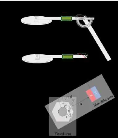
The prototype construction was made to assess the movement of the human knee joint in the sagittal plane, fixing its structure laterally to the leg. It consists of two aluminum rods, representing the goniometer arms, with a set of sensors monitored by a microcontrolled system. One of the rods must be fixed in the thigh region and the other in the calf, positioning the joint of the rods parallel to the knee.

For characterization and experimental validation, one of the prototype arms had its extremity fixed to a cylindrical basis and the other remained mobile. Both arms were connected through an axis, being that on one side, the axis has a limiter with a hexagonal section and on the other, hexagonal nuts for its fixation.

Three Hall effect sensors, model 49E, were used, fixed on the sides of the hexagonal limiter. Each sensor was fixed in the center of one of these sides, at a distance d between the end of one sensor and the other, forming angles α of 120º between the sensors. These were connected to an Atmega 168 Nano microcontroller, attached to the side of the fixed arm. A 16x2 LCD, a pushbutton, and a resistor were connected to the microcontroller. A protractor was also fixed on the external face of the movable arm to assist in the process of characterizing and evaluating the measurements of the sensors.

To insert a magnetic field close to the sensors, a rectangular edge magnet was fixed on the movable arm close to the articulation axis, with its north pole facing the sensors' face. By keeping the two arms connected on the same axis, a distance x between the sensors and the magnet was determined. The distance x was empirically chosen according to the sensitivity of the sensors and the magnetic field of the magnet (unknown), to avoid saturation of the sensor due to excessive proximity or lack of sensitivity for a very long distance. After a previous analysis, this distance x was varied between 0.1 mm and 4 mm

and it was found that the distance of x = 2 mm was the one that presented the best variation of values, avoiding the saturation of the sensors.

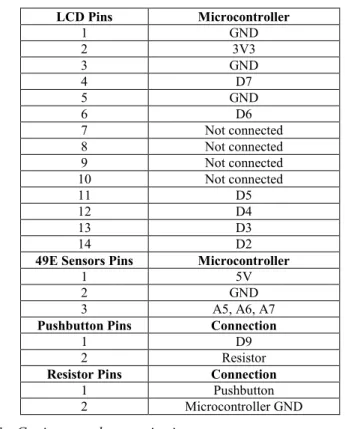
Figure 5 shows the physical structure of the prototype. In Figure 5a) there is the representation of the complete prototype; in Figure 5b), the representation of the fixed arm of the prototype; and in Figure 5c), the positioning of the sensors in relation to the articulation and the magnet fixed on the movable arm. Figure 6 shows the electronic diagram with the connections made between the microcontroller, the LCD, the sensors, the resistor, and the pushbutton. Table 1 presents, in detail, the connections shown in Figure 6 for the prototype's operation.

Figure 5: Goniometer prototype, where a) contain the complete prototype presentation, b) contain the fixed arm representation, and c) fixing position of the magnet and sensors.

Figure 6: Connections diagram between the microcontroller, the LCD, the sensors, the resistor, and the pushbutton.

(4)

JOURNAL OF APPLIED INSTRUMENTATION AND CONTROL 4 Table 1: Component connections for prototype operation

LCD Pins Microcontroller 1 GND 2 3V3 3 GND 4 D7 5 GND 6 D6 7 Not connected 8 Not connected 9 Not connected 10 Not connected 11 D5 12 D4 13 D3 14 D2

49E Sensors Pins Microcontroller

1 5V

2 GND

3 A5, A6, A7

Pushbutton Pins Connection

1 D9

2 Resistor

Resistor Pins Connection

1 Pushbutton

2 Microcontroller GND C. Goniometer characterization

As the proposal is to make a goniometer of the knee joint, the variation of the angles in the system could be from 0º to 140º [1]. However, in order to have a more complete analysis of the sensor’s response, it was decided to make a variation from 0º to 180º. The acquisition was made twenty times, varying the angles every 5º. The average of the twenty acquisitions for the three sensors was calculated. Table 2 shows these average values, in Gauss.

Table 2: Average values read by the sensors Angle Average - Sensors Angle Average - Sensors

1 2 3 1 2 3 0º 630 528 527 95º 548 794 555 5º 660 529 527 100º 539 795 566 10º 691 530 527 105º 532 787 581 15º 723 532 527 110º 527 771 598 20º 752 535 527 115º 524 748 621 25º 775 539 527 120º 522 721 647 30º 791 544 527 125º 520 692 676 35º 797 550 528 130º 519 662 708 40º 795 559 528 135º 518 635 738 45º 783 571 528 140º 517 611 765 50º 764 586 528 145º 517 592 786 55º 736 607 529 150º 516 576 800 60º 708 629 530 155º 516 564 805 65º 676 656 531 160º 516 554 801 70º 645 685 532 165º 516 547 788 75º 617 716 535 170º 516 541 768 80º 593 745 538 175º 516 537 741 85º 574 768 542 180º 516 534 710 90º 559 785 548

To evaluate the measurement curves of the sensors, the average values for each sensor were normalized. The results obtained are presented in Figure 7 graphically, where the normalized mean values and their standard deviations are present.

Figure 7: Normalized measures for the three sensors. Based on Figure 7, it can be stated that the waveforms of the sensor measurements have a shape equivalent to the normal (Gaussian) distribution and, therefore, are symmetrical in relation to its center, where its greatest amplitude value is found.

By determining the maximum points of the measurements, it was possible to check if the sensors were positioned symmetrically. The more symmetrical the positioning of the sensors, the smaller the error in estimating the angle. To evaluate this symmetry, if the curve for the first sensor had a certain lag in relation to the second, and if the curve for the second sensor had the same lag in relation to the third, it can be said that the sensors are symmetrical. An offset value θ of 61.7º between sensors 1 and 2 was reached and a θ value of 57.3º between sensors 2 and 3.

The offset values found also serve as a basis for finding the equations for the curves of sensors 1 and 3, after obtaining the equation for the curve of sensor 2. The curve of sensor 2 was used as a basis because there is a wider range of significant points compared to the curves of the other sensors.

To simplify the equation, it was decided to obtain the equation only for the case of 0º to 140º, because the prototype is aimed at the application of the knee joint goniometer. A region of the sensor 2 curve was selected to obtain, through a polynomial approximation of order 3, a relationship between the values measured by the sensors and an equivalent angle. Besides, as previously mentioned, an offset was applied to the equation for the curve to have the values for sensors 1 and 3. Figure 8 shows each region used for the sensor curves. Equation (2) that better interpolates the points of the selected curve section related to sensor 2 is:

3 2

( ) 115,6073 200,7526 155,4548 24,1188

f x  x  x  x  (2)

To determine which values will be used in the equation (for sensor 1, 2, or 3) and the offset angle θ, these conditional situations were analyzed:

 If the value of sensor 1 is greater than or equal to the value of sensor 2 and the value of sensor 2 is less than

(5)

JOURNAL OF APPLIED INSTRUMENTATION AND CONTROL 5 or equal to the threshold, use the values read by sensor

1 and θ = - 61.7º;

 If the value of sensor 2 is greater than the threshold and the value of sensor 3 is less than or equal to the threshold, use the values read by sensor 2 and θ = 0º;  If the value of sensor 3 is greater than the threshold,

use the values read by sensor 3 and θ = + 57.3º. The values of θ, in this case, are not the same due to any slight difference in positioning when fixing the sensors.

Figure 8: Normalized measures for the three sensors, with emphasis on the regions used in the equation.

The threshold value was obtained through the normalized amplitude value read by sensor 2 (0.0823) for the 35º angle. This signals amplitude value was chosen because that is when the sensors start to show greater variation in their responses, as can be seen in Figure 9.

Figure 9: Normalized measures for the three sensors, with emphasis on the threshold point.

D. Operation and Calibration

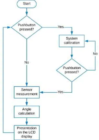
With all the steps described in the characterization process carried out, a program was implemented in the microcontroller to calibrate the system, perform the measurement of the sensors, estimate a corresponding angle value and present this value on the LCD. The flow chart of this program is shown in Figure 10. This program has an infinite loop and will only stop working if the prototype is turned off.

To start using the system, the user must carry out the calibration of the system, placing the mobile arm at 0º and pressing a pushbutton. Then, the user must move the movable arm 140º and at the end of the movement press the pushbutton

again. After this calibration step, the system is available to measure the angles, showing the estimated values on the LCD.

Figure 10: Flow chart of the goniometer program implemented in the microcontroller.

V. RESULTS AND DISCUSSION

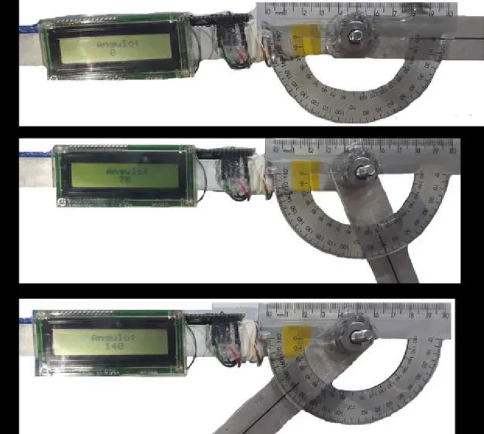
Beyond previous results already presented in the sensor characterization stage, Figure 11 shows examples of measurements made with the goniometer for 0º, 70º and 140º. Through this figure, it can be seen that for these angles, the prototype presented the expected results.

To make a more complete analysis of the error obtained by the digitization and equation process, the relationship between the angle observed in the protractor and the angle presented by the device was evaluated. Twenty acquisitions were made, varying the angle every 5º and after these acquisitions, it was evaluated for the measured angles, what was the maximum error obtained, according to equation (3), in which the maximum absolute value is calculated between the difference between θmeasured (vector containing the twenty measured values for each angle) and θreal (expected value for this angle).





_{1 20}

max measured _x real

Error max   (3)

Table 3 presents the results obtained for the maximum error values. Evaluating the table, it is observed that the maximum error obtained by the digitization and equation process for the developed prototype was ± 1.015º, when the 35º angle was measured.

(6)

Figure 11: Examples of measurements made with the goniometer: a) 0º, b) 70º e c) 140º.

Table 3: Maximum prototype error for the evaluated angles Angle Maximum Error Angle Maximum Error

0º 0,268 75º 0,992 5º 0,153 80º 0,640 10º 0,510 85º 0,117 15º 0,746 90º 0,213 20º 0,325 95º 0,538 25º 0,701 100º 0,458 30º 0,649 105º 0,175 35º 1,015 110º 0,117 40º 0,035 115º 0,213 45º 0,689 120º 0,173 50º 0,223 125º 0,352 55º 0,636 130º 0,803 60º 0,105 135º 1,008 65º 0,069 140º 0,526 70º 0,697

A boxplot-type graph was used to evaluate the dispersion of the maximum error values found, as shown in Figure 11. In it, we can see that most of the error values are below 0.7, in addition to the fact that that the average of the errors obtained was close to 0.5.

Figure 7: Boxplot of the dispersion of the maximum errors obtained with the goniometer prototype.

(7)

JOURNAL OF APPLIED INSTRUMENTATION AND CONTROL 7 VI. FINAL CONSIDERATIONS

The present work aimed to develop a prototype of a goniometer to measure the knee joint angles. In this way, it was possible to measure angles from 0º to 140º. A very important step dealt with the characterization of Hall effect sensors within the assembled system.

This characterization made it possible to estimate the angles to be measured based on the values presented by the sensors. The adopted characterization process can be improved in many aspects, in view of the difficulties encountered during its development.

Regarding the measurement of the angles with the use of the protractor, there was not a very precise system, since the measurements were made visually every 5º. As a suggestion for improvement, the use of a universal goniometer fixed to the structure to be able to measure the angles every 1º, instead of 5º.

In addition, during measurements to characterize the sensors, there was no mechanical stability in relation to the movable arm, where it should be adjusted so that it would not move on another axis than desired. It is proposed for future work to insert a bearing to couple the fixed bar and the moving bar, reducing the variations that were observed in this prototype. For the purpose of a more complete characterization system of the sensors, it is proposed to use six sensors to measure 360º.

With regard to the positioning of the magnet, it is noteworthy that by adopting a distance of 2 mm from the magnet in relation to the sensors, the signals obtained could be used in the goniometer system, unlike the case of other distances that either showed saturation or almost no variation was observed.

When handling these sensors, it is worth mentioning that because characterization is made using data of analog value, magnetic field source not completely determined and geometric/physical variations, it is considered that the prototype can present measurement errors of up to ± 1.015º. Another factor that proves this issue is in relation to the positioning of the sensors, in which has made numerous adjustments, the maximum measured offset angles was not the same between sensors 1 and 2 and sensors 2 and 3.

Finally, there is also a suggestion for future work to deepen the analysis proposed in this work in relation to the equation and determination of the threshold, aiming to minimize the measurement error, since the biggest error obtained was precisely for the angle at which the threshold was determined. For example, instead of using only one sensor's information at a time, make a pair of sensors to compensate for positioning errors. It is also suggested to compare Hall Effect sensors and inertial sensors within this application, to assess which one has the least error, mainly due to the positioning of the sensors.

REFERENCES

[1] A. P. Marques, Manual de goniometria. Barueri, SP: Editora Manole, 2003.

[2] C. C. Norkin e D. J. White, Measurement of Joint Motion, A Guide to Goniometry, 3 ed. F. A. Davis, 2003.

[3] M. L. Moore, “The Measurement of Joint Motion*: Part II: The Technic of Goniometry”, Phys. Ther., vol. 29, no 6, p. 256–264, jun. 1949, doi: 10.1093/ptj/29.6.256.

[4] G. T. Laskoski, “Desenvolvimento de um Goniômetro Telemétrico Indutivo para Aplicações Biomédicas”, Dissertação de Mestrado, Universidade Tecnológica Federal do Paraná, Curitiba, Paraná, 2010. [5] C. A. D. Turqueti, “Desenvolvimento de um Goniômetro Indutivo com

Bobinas Ortogonais para Aplicações Biomédicas”, Dissertação de Mestrado, Universidade Tecnológica Federal do Paraná, Curitiba, Paraná, 2017.

[6] E. S. Bespalov, V. V. Kurgin, e M. I. Musyankov, “The ways of forming the single-valued scale for the space station phase radio goniometer”, in 3rd International Conference on Satellite Communications (IEEE Cat. No.98TH8392), Moscow, Russia, 1998, p. 128–130, doi: 10.1109/ICSC.1998.741382.

[7] W. Hong, “Design of a more powerful mini-type tripod head for laser goniometer based on CPLD”, in 2017 Chinese Automation Congress (CAC), Jinan, out. 2017, p. 3987–3990, doi: 10.1109/CAC.2017.8243477. [8] M. Donno, E. Palange, F. Di Nicola, G. Bucci, e F. Ciancetta, “A Flexible Optical Fiber Goniometer For Dynamic Angular Measurements”, in 2007 IEEE Instrumentation & Measurement Technology Conference IMTC 2007, Warsaw, Poland, maio 2007, p. 1–5, doi: 10.1109/IMTC.2007.379176.

[9] T. Resende et al., “Universal Goniometer and smartphone app for evaluation of elbow joint motion: Reproducibility analysis”, in 2017 International Conference on Virtual Rehabilitation (ICVR), Montreal, QC, Canada, jun. 2017, p. 1–2, doi: 10.1109/ICVR.2017.8007528.

[10] M. S. Barreiro, A. F. Frere, N. E. M. Theodorio, e F. C. Amate, “Goniometer based to computer”, in Proceedings of the 25th Annual International Conference of the IEEE Engineering in Medicine and Biology Society (IEEE Cat. No.03CH37439), Cancun, Mexico, 2003, p. 3290–3293, doi: 10.1109/IEMBS.2003.1280847.

[11] N. Carbonaro, G. D. Mura, F. Lorussi, R. Paradiso, D. De Rossi, e A. Tognetti, “Exploiting Wearable Goniometer Technology for Motion Sensing Gloves”, IEEE J. Biomed. Health Inform., vol. 18, no 6, p. 1788– 1795, nov. 2014, doi: 10.1109/JBHI.2014.2324293.

[12] G. em S. ACE, Manual de Goniometria - Medição dos Ângulos Articulares. .

[13] E. L. Camargo Jr., F. A. Farinelli, e S. L. Stevan Jr., “O Efeito Hall e suas Aplicações em Sensoriamento”, Ponta Grossa, Paraná, 2018, p. 5. [14] A. L. Rezende Neto, A. Magagnin Júnior, E. C. R. Neiva, e R. Farinhaki,

“Sistema de Medição de Campo Magnético Baseado no Efeito Hall e Arduino”, Monografia, Universidade Tecnológica Federal do Paraná, Curitiba, Paraná, 2010.

[15] D. Halliday, R. Resnick, e J. Walker, Fundamentos de física: volume 3 : eletromagnetismo. LTC, 2008.

[16] YANGZHOU POSITIONING TECH. CO., LTD, “49E Hall-Effect Linear

Position Sensor”, 06/10.

http://p.globalsources.com/IMAGES/PDT/SPEC/440/K1139513440.pdf.

Received: 04 June 2020; Accepted: 28 September 2020; Published: 29 September 2020

(8)

Protótipo de Goniômetro da Articulação do Joelho

utilizando Sensores de Efeito Hall

Resumo — O trabalho apresenta o desenvolvimento de um protótipo de goniômetro para realizar as medições de articulação do joelho. Foram utilizados três sensores de efeito Hall posicionados a 120º entre si, em conjunto com um imã de extremidade retangular posicionado externamente a estes sensores. Descreve-se no trabalho todo o processo de caracterização dos sensores dentro do sistema, além da estrutura do goniômetro. Como resultados obteve-se a medição de ângulos de 0º a 140º, com um erro máximo de medição de 1,015º. Por fim, concluiu-se que o protótipo tornou possível a medição dos ângulos nos valores propostos, além de trazer diversas propostas de melhorias no sistema para trabalhos futuros, como o posicionamento dos sensores, melhorar a estrutura de validação dos ângulos, entre outros.

Palavras-chave — goniômetro do joelho, sensores de Efeito Hall, caracterização.