Eric Vaz1 Jessica Miki2 Teresa de Noronha3 Michael Cusimano4 AbstrAct
In this paper an empirical assessment of injury patterns is supplied as an example of social endurance - resilient societies can be built by means of geographical analysis of injury data, providing better support for decision makers regarding urban safety. Preventing road traffic collisions with vulnerable road users, such as pedestrians, could help mitigate significant loses and improve infrastructure planning. In this sense, the geographical aspects of injury prevention are of clear spatial analog, and should be tested regarding the carrying capacity of urban areas as well as vulnerability for growing urban regions. The application of open source development tool for spatial analysis research in health studies is addressed. The study aims to create a framework of available open source tools through Python that enable better decision making through a systematic review of existing tools for spatial analysis. Methodologically, spatial autocorrelation indices are tested as well as influential variables are brought forward to establish a better understanding of the incremental concern of injuries in rural areas, in general, and in the Greater Toronto Area, in particular. By using Python Library for Spatial Analysis (PySAL), an integrative vision of assessing a growing epidemiological concern of injuries in Toronto, one of North America’s fastest growing economic metropolises is offered. In this sense, this study promotes the use of PySAL and open source toolsets for integrating spatial analysis and geographical analysis for health practitioners. The novelty and capabilities of open source tools through methods such as PySAL allow for a cost efficiency as well as give planning an easier methodological toolbox for advances spatial modelling techniques.
Keywords: Open Source, Spatial Analysis, Resilience, Geographic Analysis, Spatial Decision Support Systems, Python.
JEL Classification: I10, I18, C31
1. IntroductIon
Since the late 1960s GIS and spatial analysis statistics has been used to effectively model, study, and interpret results of geographic phenomena with spatial dimensions and associated attributes (Burrough, 2001). They are commonly used in the City of Toronto (2014) for informed and enhanced decision making through: (i) evaluating suitability and capability,
1 Department of Geography and Environmental Studies, Ryerson University, Toronto, ON, Canada. Research Centre for Spatial and Organizational Dynamics, University of the Algarve, Faro Portugal. [email protected]
2 Department of Geography and Environmental Studies, Ryerson University, Toronto, ON, Canada. [email protected]
3 Faculty of Economics, University of the Algarve, Faro, Portugal. Research Centre for Spatial and Organizational Dynamics, University of the Algarve, Faro Portugal. [email protected]
(ii) estimating and predicting, and, (iii) interpreting and reorganizing of information. In this sense, further implementation of geographical analysis can be brought by integration of spatial analysis standards, where implementation of better decisions geared towards protection of citizens and fostering better analytics may have a leading role in mitigation of injuries (Vaz et al., 2016). Cost efficiency of exploring novel techniques for adapting new tools must be considered, given the budgetary constraints of commercial software licenses, open source may become important analytical tools to mitigate the concerns of injuries in a growing region.
Every year close to 1 per cent of Canadians are injured in a road traffic incident (Andrey, 2000). Within Canada, Toronto has the highest motor vehicle collision injury rate, in the past decade alone, there were more than 20 deaths per year, and the pedestrian and cyclists’ collisions with cars generated direct costs of $62 million (IndEco Strategic Consulting Inc., 2012). Road traffic accidents strain social, infrastructure, and health care systems and represent thus an incremental cost to society. Per Transportation Canada (2014) in 2009 a total of 2009 fatalities and 1145 serious injuries were registered in road traffic accidents. The city of Toronto (Toronto Public Health, 2012) identified road traffic accidents as the leading cause of death in youth for 2010. Approximately 25% of all road traffic fatalities in Canada are described as vulnerable road users, with 13% of all fatalities being pedestrians (Transport Canada, 2014).
We present three distinct spatial analytical applications as to address the complexity of injuries within the study region. Our paper is structured as follows: (i) In a first section we test the capability to visualize and describe collision information and visualize the data. Due to the sensitivity of the health information, collision points were aggregated as injury counts within Toronto neighbourhoods. The second part focuses on efficient assessment of high and low descriptives of collision neighbourhoods, followed by applications of spatial autocorrelation through the implementation of Global and Local Moran’s I statistics. Finally, and most importantly, we establish a framework for Toronto on the socio-economic profile of neighbourhoods, adopting a Geographically Weighted Regression (GWR) model. For the definition of the socioeconomic study the factors were derived by the city of Toronto’s open data portal, much in line with the avenue this study procures, in addressing a open source framework for spatial analysis. The following sections lead to a discussion of findings as well as conclusions, were we incorporate the broader picture of applications within public health participation with more advanced spatial analysis tools to efficiently plan regions.
Ours is a Python based modelling approach. These have proven efficient to answer social, economic and environmental concerns. While many of these programming languages require an advanced knowledge of programming and scripting making the learning curve steep, novel geocomputational methods are steering towards simplified syntaxes that allow laymen work together with experts and bring efficient and simple solutions. The Python Spatial Analysis Library (PySAL) was used to develop the study and generate tools to widen scientific applications (Rey et al., 2008). This paper takes a systematic approach to understand the contribution of such tools for public health. PySAL is used as to integrate spatial analysis methods and assessing this instrument for the applied public health sector. Open source software and practices offer major advantages for applying spatial analysis to multifaceted research activities. The variety of open source tool sets can be used to further explore, educate, and empower researchers and general users. The openness cultivates a greater culture of knowledge sharing through transparent, adaptable, portable, and modularity coded processes (Ertz, Rey & Joost, 2014). PySAL and other open source software can be freely installed on personal and institutional devices, offering greater access than traditional predesigned software packages. Within a growing body of digital data, where spatiotemporal availability and locational accuracy is exponentially growing, such tools may
set new benchmarks for the general public as well as very specific silos of application. This study focused on car collisions and the resulting injuries on pedestrians. The complexity of this problem represents the ideal laboratory to forward a clear geographical analytical application of a concern that has not been explored in the Greater Toronto Area from a spatial analysis stance.
2. study AreA
The study will focus on the neighbourhoods of the municipality of Toronto. In the year 2011, the city of Toronto had an estimated population of 2,615,060 residents (Statistics Canada, 2014). The City of Toronto composes of 630.21 square kilometers, and has a population density of 4,150 persons per square kilometres (Statistics Canada, 2014). The population densities are significantly greater than the national value of 4 persons per square kilometers (Statistics Canada, 2014), and creates a strong activity center for Canada. The Greater Toronto Marketing Alliance (2011) describes the Greater Toronto Area as the fourth largest business and manufacturing region in North America. This economic region supports the second largest automotive centre in North America, and 21 out of Canada’s top 30 law firms. These are key industries that can benefit from collision mapping and prevention to improve automotive safety and insurance claims. Improving road safety has long established economical and holistic benefits as the 25-year capital program includes a $50 billion rapid transit plan with Metrolinx to spread the transit systems within 2 kilometers within 80% of the city’s residents (Greater Toronto Marketing Alliance, 2011). Improving transit infrastructure is a key priority as regional planning will have to accommodate for demographic changes. A prominent population trend observed by Statistics Canada (2015) is the increasing immigrant population that maintains Toronto’s population and urban growth (Vaz & Arsanjani, 2016). Their report suggests that immigrant population growth will have an impact on the regional infrastructure and planning demands (Vaz et al., 2016). The growth in population and development can be observed through the 10.5% growth of private dwellings, to 1,989,705 Toronto dwellings, from 2006 to 2011 (Statistics Canada, 2014). This is a larger growth than the national change of 7.1% in private dwellings usually occupied by residents (Statistics Canada, 2014), and show cases Toronto’s strong demand for strategic and sustainable infrastructure planning. In order to generate more information for better decision and policy making in the dynamic city of Toronto the neighbourhoods will be used as they study boundaries.
3. dAtA
Collision data from 2002 to 2013 were collected by the Canadian Institute for Health Information (CIHI). Inconsistent entries for the year 2013 are also included, and lack geographical referenced coordinates as well as other key values. The information helps to support effective healthcare systems management, distribute health information, and raise awareness for public health initiatives (Canadian Institute for Health Information, 2015). As health data contains sensitive information rounding values can be used to generalize the information. In this data set International Classification of Diseases (ICD) has been used to describe the injury incident. The ICD are World Heath Organization (2015) standard diagnostic tools used in epidemiology, health management, and clinical processes to classify health problems by type and severity. These ICD tags were used to identify and select the desired collision entries for this analysis. ICDs for motor vehicle collisions with pedestrian, and motor vehicle collisions with pedestrians for 2010 were selected using a SQL query
and exported into separate data sheets. The georeferencing information from the data sheets, described as ‘x’ and ‘y’ coordinate values, was input into ArcGIS for visualization and to spatially join the collision incidents to their respective Toronto neighbourhoods. Neighbourhood shapefiles were obtained from the City of Toronto’s Open Data catalogue (Toronto Open). The City of Toronto (2015) and Statistics Canada census tracts use these neighbourhood boundaries to statistically report and perform longitudinal studies as the boundaries do not change over time. Neighbourhoods offered a meaningful geographic area for effective community planning and aggregation level for the health data. Neighbourhoods built from the Statistics Canada census tracts cover several city blocks with 7,000 to 10,000 residents, and respect existing boundaries (The City of Toronto, 2015a). These boundaries are used for the Wellbeing Toronto web application, released to also help users visualize and evaluate community social development datasets (The City of Toronto, 2015b). The year 2010 was chosen as it complements the study completed by the City of Toronto and associated public health analysis. As a guiding framework for spatial analysis of public health data it was important to utilize open source data sets and tools. All the methodology and data steps were completed in open sours programs. The socio-economic data was collected from Toronto open data portal. As identified in the literature review, gender, education levels, employment status, annual income, and age can influence the number and frequency of pedestrian road collisions. Socio-demographic data was collected from the Toronto Open. The data was collected from the 2006 and 2011 census, and processed into Toronto neighbourhood boundaries (The City of Toronto, 2014). The neighbourhood identity numbers were used to join socio-demographic files to the geographic shapefiles of Toronto neighbourhoods, also provided by the Toronto Open data team. The data has been processed from the census values, and have been processed by Statistics Canada (2010 source) to normalize the data. To identify any correlated socio-economic factors that may add statistic bias to the study analysis the database file with the determinant factors and neighbourhood identities were standardized and correlated through R studio statistic software. R studio is another open source development platform that utilizes coding for statistical analysis.
4. Methods
The study outlines an effective and feasible framework for spatially analyzing health data. It utilizes PySAL and R packages, followed by QGIS for visualization purposes. Initially QGIS is used to map collision frequency of Toronto neighbourhoods. Global spatial autocorrelation was then generated in PySAL to identify patters of collision frequency and severity. PySAL was also used for the local Moran’s I spatial autocorrelation analysis to identify patterns of collisions correlation within the neighbourhoods. To identify any explanatory factors R studio was used to select socio-economic factors for the geographic weighted regression (GRW) analysis testing in PySAL. PySAL has multiple geographical weighted regression models available. To maintain simplicity for users, the Ordinal Lease Squares (OLS) with geographic weight matrix method was used to measure the similarity of the socio-economic factors to model the collision frequencies. The results can be used to identify potentially vulnerable road users and areas that can be targeted for improving road safety. The framework can then be used to help introduce spatial analysis tools into healthcare analysis, as well as other industries that would greatly benefit from affordable and accessible toolsets.
4.1 Visualizing neighbourhood collision incidents
Before using the code based statistical packages it is useful to visualize the collision data. Map visualization helps users evaluate geographic datasets and better comprehend community
health indicators (The City of Toronto, 2015b). This initial objective was completed through spatially joining collisions to their respective neighbourhoods and demographic profiles. From the database file as a spreadsheet or attribute table ArcMap application, the rate of traffic collisions per residential population count could be calculated (Table 1).
table 1. top 13 collision counts in neighbourhoods from 2010 neighbourhood
identity number neighbourhood name residential population Pedestrian collisions collision frequency rate
collisions per 1000 residents
1 West Humber-Clairville 32265 23 0.0007 1
136 West hill 25635 21 0.0008 1 70 south riverdale 24430 19 0.0008 1 73 Moss Park 15480 18 0.0012 1 116 Steeles 24705 18 0.0007 1 132 Malvern 44315 18 0.0004 0 75 Church-Yonge Corridor 24370 17 0.0007 1 126 Dorset Park 24365 17 0.0007 1 137 Woburn 40845 17 0.0004 0 2 Mount Olive- Silverstone-Jamestown 32130 16 0.0005 0 26 Downsview-Roding-CFB 32010 16 0.0005 0 93 Dovercourt-Wallace Emerson-Juncti 34725 16 0.0005 0 129 Agincourt North 30160 16 0.0005 1
Source: Own Elaboration
In order to make the rate more comparable the frequency of collisions per resident was then applied to identify how many collisions would occur for every 1,000 residents. The largest 10 values of collision count and collision frequencies was organized into table 2. The summary table demonstrates that neighbourhoods with high collision counts do not consistently have a high frequency of residential and motor vehicle collisions. Of the highest values observed in 13 and 11 neighbourhoods, only the West Hill (136), South Riverdale (70), and Moss Park (73) have high collision counts and frequencies. This may be because Toronto has a high transient population that is not counted within the residential population. Toronto has a high commuting population, and as previously identified many trips can be achieved through active transportation modes. Research also suggests that in areas with high active transportation concentration there are less motor vehicles to cause collisions. The map and regression analysis can help to further identify any contributing collision factors and areas that can be targeted for improving conditions.
table 2. top 11 collision frequencies in neighbourhoods from 2010 neighbourhood
identity number neighbourhood name residential population Pedestrian collisions collision frequency rate
collisions per 1000 residents
73 Moss Park 15480 18 0.0012 1
110 Keelesdale-Eglin-ton West 11225 11 0.0010 1
113 Weston 16470 14 0.0009 1
22 Humbermede 14780 13 0.0009 1
114 Lambton Baby Point 7780 7 0.0009 1
112 Beechbor-ough-Greenbrook 6530 6 0.0009 1 136 West hill 25635 21 0.0008 1 70 south riverdale 24430 19 0.0008 1 44 Flemingdon Park 21290 16 0.0008 1 30 Brookhaven-Ames-bury 17325 13 0.0008 1 86 Roncesvalles 14650 11 0.0008 1
Source: Own Elaboration
The collision counts and frequencies were mapped in ArcMap to produce figures one and two. Figure 1 maps the collision counts in each neighbourhood, while figure 2 maps the rate of collisions over the residential population. The maps effectively colour the regions with equal interval values that can be used to start to generate trend conceptual trends. Without more information, an accurate conclusion cannot be made about the pedestrian and vehicle collisions, a more thorough statistical analysis is needed to determine if the collision distribution is random or has any contributing factors.
Figure 1. ArcMap generated counts of the 2010 reported vehicle and pedestrian collisions in toronto neighbourhoods
Source: Own Elaboration
Figure 2. ArcMap generated residential frequencies of the 2010 reported vehicle and pedestrian collisions and neighbourhoods’ residential population
4.2 spatial weights in PysAL
In order to effectively run a spatial analysis, spatial weights will have to be used to give the location values of the data set a contextual meaning. As PySAL Developers (2015) data, spatial weights are central components for some spatial analysis techniques as the spatial weights matrix describes the potential for interaction between observations given their locations. Within the PySAL environment, spatial weight matrices can be generated through contiguity based weights, distance based weights, and kernel weights. In order to store the large datasets with a full matrix, and mitigate memory constraints, PySAL stores the matrices in two main dictionaries, respectively for neighbours and weights of each observation (PySAL Developers, 2014). This allows for PySAL to effectively generate weights for and accurate global spatial autocorrelation analysis. PySAL also allows for topology to accurately represent by generating spatial weights from shapefiles, as empirical research and non-topological vector data can be used to construct the weights before an analysis (PySAL Developers, 2014).
The queen contiguity spatial weight matrix was used to calculate the Moran’s I value. The Geoda workbook by Anselin (2005) outlines that the queen contiguity is effective for areal or polygon data. This matrix type was able to include more wards in the analysis than the alternative spatial weight matrixes. In order to maintain accuracy, the weight matrix was generated from the shapefile.
4.3 Global spatial Autocorrelation
Spatial autocorrelation can be used to identify spatial patterns and geographic relationships between features in space. Spatial autocorrelation techniques have been developed and used to measure non-random spatial patterns of attribute values (PySAL Developers, 2014). Two commonly used techniques focus on observing the global spatial autocorrelation and the local spatial autocorrelation. Global spatial autocorrelation reviews variable values to identify any patterns of clustering across the study area (Chun & Griffith, 2013). Local spatial autocorrelation reviews regions within global patterns of clusters (Bivand, 2015), described as hot or cold spots for high and low respective values (Ord & Getis, 1995). Relationships that cluster similar values have a positive autocorrelation; while negative autocorrelations have clusters of dissimilar values (PySAL Developers, 2014). If there is not a significantly positive or negative correlation, then the arrangement of values can be concluded as random.
Ord-Getis (1995) and Chun and Griffith (2013) identify that global Moran’s I can be used to effectively measure the correlation of spatial features. PySAL’s Moran’s I for global spatial autocorrelation has been described in equation 1. Where n is the total number of features, y the attribute, the attribute’s deviation from feature i, and i’s mean generates zi (equation 2),
wi,jis the spatial weight between features i and j, S0is the aggregate of all the spatial weights, calculated as a Moran’s I value from -1 to 1. A Moran’s I value of 1 indicates that features are positive autocorrelation; and a -1 value indicates that features are dispersed in a negative spatial autocorrelation (Bivand, 2015). While a value of 0 suggests that features have no significant relationship, and are randomly distributed with no spatial autocorrelation. The significance of the Moran’s I can be described through the z-score value. A z-score greater than 1.96 or less than -1.96 concludes that the spatial autocorrelation has a significance level of 5% (0.05) (ESRI, 2009). If the significance level is above 5% it is unlikely to be a result of a random distribution. The Moran’s I pseudo significance level (p-value) can also be used to determine if a sample has statistical significance (Anselin, Exploring Spatial Data with GeoDA: A Workbook, 2005); with a confidence level of less than 0.05. If the p-value
is greater than 0.05 then the sample is random and does not have a statistically significant spatial autocorrelation.
equation 1. Global Moran’s I (PysAL developers, 2014)
equation 2. Global Moran’s I attribute information (PysAL, 2014)
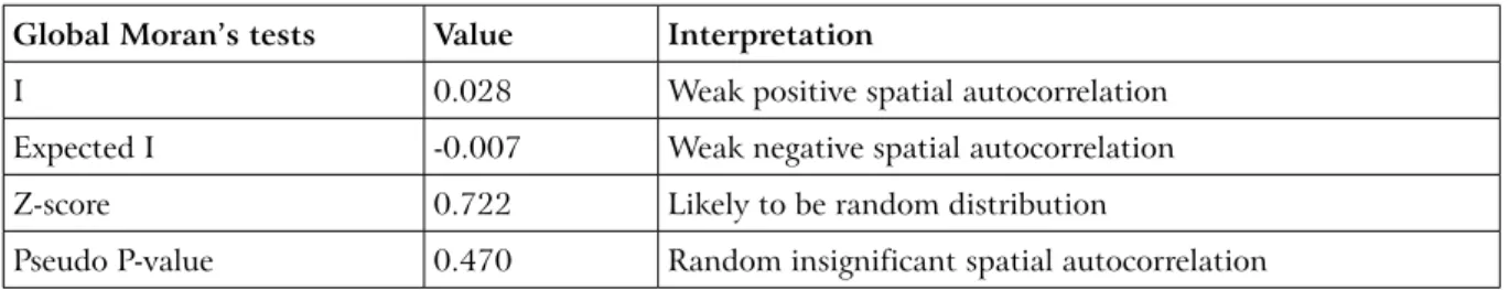
To further identify statistically significant collision clustered areas, objective two utilized global and local spatial autocorrelation Moran’s I analyses. The results (table 3) suggest that the collisions occur randomly with low spatial autocorrelation patterning. Global significance from the instance was measured through the z-score as 0.72, and the positive spatial autocorrelation has a 0.47 p-value confidence, suggesting that the pattern is randomly distributed. The numeric values are extremely direct in conveying the low statistical significance of the collision incidents. PySAL returned 14 significant digits, offering a very precise and statistical analysis for a variety of study applications.
table 3. Global Moran’s I summary statistics Global Moran’s tests Value Interpretation
I 0.028 Weak positive spatial autocorrelation
Expected I -0.007 Weak negative spatial autocorrelation
Z-score 0.722 Likely to be random distribution
Pseudo P-value 0.470 Random insignificant spatial autocorrelation
Source: Own Elaboration
4.4 Local spatial Autocorrelation
To utilize PySAL in localized clusters local Moran’s I statistical analysis was generated. Local Moran’s I can be used to evaluate local measures of spatial variation and association (Anselin, 1995). The local Moran’s I counts the collisions within a dissemination area and identifies if they are high or low cluster values. PySAL local Moran’s I (equation 3) uses the same variables as the global statistic, described above.
equation 3. Local Moran’s I (PysAL, 2014)
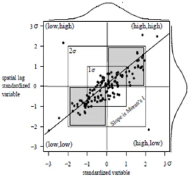
PySAL generates Local Indicators of Spatial Autocorrelation (LISA) statistics to quantitatively measure local spatial autocorrelation for Moran’s I tests. LISA was used to indicate how many points were statistically significant (less than 0.05), with inferences of the collision values calculated through pseudo-p values for each LISA. The “Numpy” module
extension was used to identify significant LISAs and then the indexing was used to find the quadrant of a Moran’s scatter plot where each of the significant values would be placed. Figure 3 displays a positive autocorrelation of standardized sample of the scatter-plot, where the variable of interest (collisions) average against the neighboring values. The Moran’s I value would be the slope of the line of best fit in the scatter plot (Ward & Gleditsch, 2007).
Figure 3. standardized Moran’s I scatter plot (Ward & Gleditsch, 2007)
Source: Own Elaboration
When running the local Moran’s, I analysed all 140 wards were considered, then 16 statistically significant wards were identified through their LISA p-values (less than 0.05). These significant wards were selected though PySAL, and their respective plot quadrants were returned. As the majority of the significant values are in the third quadrant there is a significant amount of low values surrounding low observations. It can be concluded that the collisions are not concentrated in one geographic region. The regression analysis can be used to identify if there are any contributing factors within the neighbourhood.
4.5 Geographic ordinal Lease squares regression
Spatial regression was used to identify any correlation between socio-demographic factors and collision rates. Factors that may influence collision rates include levels of; gender, age, education, income, occupation (get stats). In order to compare the collision frequency and socioeconomic factors the samples were transformed into percentages of the ward population. In PySAL spatial regression can be diagnosed through Anselin, Bera, Florax and Yoon (1996) Lagrange multiplier (LM) test. They used the Jarque-Bera method to develop a test for spatial dependency and heteroskedasticity that can be applied in socio-economic studies and urban environments.
In PySAL the Ordinal Least Square (OLS) spatial regression analysis is a Geographic Weighted Regression (GRW) analysis used to test for spatial autocorrelation of the collisions and socio-demographic variables. The OLS has been adapted with geographic weighted regression (GRW) considerations for local parameters, rather than global parameters to calculate the strength of fit a model has to a hypothesis (Gao & Li, 2011). The GWR
equation calculates R2 as the goodness of fit from 0 to 1, where 1 and high values represent
a better fit model than 0 and low values. The geographic OLS (GOLS) statistics were generated from the queen weight matrix was used in Moran’s I method to optimize the ward polygons. From the CSV file of the collisions (dependant) and independent variables were transformed into nx1 (dependant) and nx2 (independent or explanatory variables) arrays. Spatial weight from the Moran’s I statistics was used to weight the CVS objects; no row-standardization was applied as the samples are already estimated.
The GOLS analysis offers insight into factors that contribute to collision rates. The R2
and the adjusted R2 value of 0.52 and 0.49 respectively, suggest that the model is not a strong
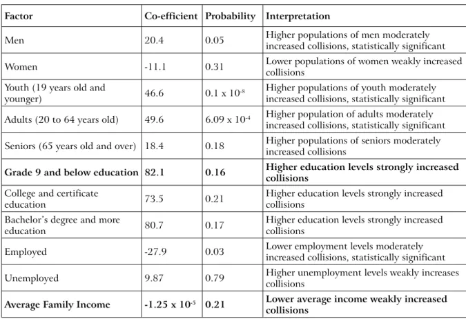
fit for the study. In this simple application GOLS was applied to several different socio-economic factors to demonstrate the PySAL process. The socio-socio-economic features included estimated populations of age groups, average family income, education levels, gender, and employment statuses. Each factor’s correlation with collision injuries were measured through the GOLS analysis (table 4). The co-efficient and probability values suggest the strength and type of relationship the variables have on collision frequency (ESRI, 2009). Complimentary to the review of literature, the model identifies that collisions will increase by 82counts for every one percent of growth in the population that has a grade 9 and below education. All education based factors had strong positive relationship with the collision counts, they had the largest respective coefficient value of all explanatory factors. Average family income had the smallest coefficient value, and negatively affected the collision frequency. Comparatively, all the other factors have a moderate influence on the collision counts; when all other variables remain constant (ESRI, 2009). Although only male, youth, adults, and employment rates had statistically significant probabilities that the explanatory factors were not random outcomes. All the other probabilities are greater than the designated 0.05 p-value, and may be random outcomes of this incident.
table 4. GoLs collision Factor summary statistics Factor co-efficient Probability Interpretation
Men 20.4 0.05 Higher populations of men moderately increased collisions, statistically significant
Women -11.1 0.31 Lower populations of women weakly increased collisions
Youth (19 years old and
younger) 46.6 0.1 x 10⁻⁸ Higher populations of youth moderately increased collisions, statistically significant
Adults (20 to 64 years old) 49.6 6.09 x 10⁻⁴ Higher population of adults moderately
increased collisions, statistically significant Seniors (65 years old and over) 18.4 0.18 Higher populations of seniors moderately increased collisions
Grade 9 and below education 82.1 0.16 higher education levels strongly increased collisions
College and certificate
education 73.5 0.21 Higher education levels strongly increased collisions
Bachelor’s degree and more
education 80.7 0.17 Higher education levels strongly increased collisions
Employed -27.9 0.03 Lower employment levels moderately increased collisions, statistically significant
Unemployed 9.87 0.79 Higher unemployment levels weakly increases collisions
Average Family Income -1.25 x 10⁻⁵ 0.21 Lower average income weakly increased
collisions
4.6 PysAL regression diagnostics
In the OLS regression report diagnostic statistics are also included. The diagnostic statistics can be used to quantify the confidence the GOLS method has in modeling the collision patterns and factors. As the multicollinearity condition number is 779.33 and the regression diagnostic statistics are irregular, it can be concluded that this model offers a weak fitted regression analysis (table 5). The Jarque-Bera normality of errors (JB) describes if residuals are normally distributed; a value under 0.05 (probability) identifies that the residuals are not normally distributed and the results have unreliable model misspecification (ESRI, 2009). In this incident the JB has a p-value of 0.29, meaning the GOLS model results are trustworthy and can be used to describe linear regression correlations. Supplementary to this diagnostic statistic, the Breusch-Pagan (BP) and Koenker-Bassett (KB) tests diagnostics for heteroskedasticity (Bivand, 2015). The random coefficients can be used to determine if the independent (explanatory) variables have a consistent relationship with the collision (dependant) counts (ESRI, 2009). As the BP p-value is significant (0.04) and the KB is not significant (0.11) the heteroskedasticity and non-stationary conditions cannot confidently be accepted.
table 5. GoLs regression diagnostics summary
test degrees of freedom statistical value P-value Interpretation
Jarque-Bera normality of
errors 2 2.41 0.29 Acceptable GOLS report
Breusch-Pagan test diagnostics for heteroskedasticity random
coefficients 11 20.3 0.04 Acceptable GOLS report
Koenker-Bassett test diagnostics for heteroskedasticity random coefficients
11 16.9 0.11 Flawed GOLS report
Source: Own Elaboration
PySAL generates multiple OLS regression statistics, as well as additional test linear regression a spatial diagnostic test can be generated. All of the PySAL LM tests run in the residuals to identify the presence of remaining spatial autocorrelation of an OLS model, and suggest an accurate spatial model (PySAL Developers, 2014). In PySAl there are 5 types of spatial models: simple and robust spatial lag; simple and robust spatial error; and joint presence of spatial lag with spatial error model (PySAL Developers, 2014). Each tests in the residuals return the statistic and p-value that can be used to identify an alternative model with a better fit for more accurate analysis (PySAL Developers, 2014).
5. dIscussIon And concLusIons
While this study explores research relevant to car collision prevention within a neighbourhood scale the methods can be adapted into areas such as physical sciences, social sciences, health, tourism, planning, tourism, and more. This study of neighbourhood collisions may contribute to the trends in net health studies for trends of public health studies are identified as: social or racial health inequalities; health policy development and disease control; sense of individual-based analysis for poor health; and exploration into GIS data (Diez Roux & Mair, 2010). These resources can be used to benefit policies and communities with targeted neighbourhood level features (Diez Roux & Mair, 2010).
Developing and active transportation network will improve infrastructure and connectivity of the participating GTA municipalities. Increased connectivity boosts the bike-ability and walkability of areas that have poor planning attributes, and associated negative effects. This planning strategy may also qualify municipalities for federal and provincial funding for long-term and larger scale building projects than previously possible. Larger scale funding and projects will have increased benefits for community and individual health (The City of Toronto, 2012). The city of Toronto (2012) describes large scale active transportation project as being able to decrease car collisions and noise pollution, while improving air quality.
The investments into improving road safety represent a small fraction of the estimated costs, and projects can be paired with other government structures for funding and strategies to control health care costs. For example, the Greater Toronto Area (GTA) municipalities can work with Metrolinx to construct and active transportation network (The City of Toronto, 2012). The City of Toronto (2012) also recommends projects for investing in active transportation infrastructure, lowering speed limits, and implementing advanced traffic signal systems. Better data collection and analysis should guide infrastructure improvements for promoting safer active transportation.
The sense of safety within a neighbourhood has been observed to positively influence the health and economic stability of an area. As forms of physical activity have positive effects on cases of mental illnesses and stress, the City of Toronto (2012) identifies stress reduction as a value-added asset of active transportation. Within Toronto, 27% of the population 15 years old and under in 2001 surveyed most days in their life were quite stressful or extremely stressful (The City of Toronto, 2012). Promoting active transportation lifestyles can introduce daily stress relieving forms of physical activity, and reduce the risk of chronic diseases (The City of Toronto, 2012). Real estate values are also dependent on the neighbourhood quality of life.
Finally, this study was designed to demonstrate the benefits of using PySAL and open source applications for spatial analysis methods. The functional method can be applied to different datasets types for exploring global and local spatial autocorrelation, and spatial regression. In this application, neighbourhood collision and wellbeing levels were examined to identify vulnerable road users and target infrastructure solutions within the neighbourhoods. The data was analyzed through python based spatial analysis library techniques, and utilized other ooen source software packages. This makes the study highly accessible to others for reviewing and building on the research presented.
Our research goals have been achieved: 1) To develop a PySAL based analysis for modeling collision condition; 2) To identify spatial patterns for injuries; 3) To measure pedestrian collisions within Toronto neighbourhoods. The first objective of spatially enabling the collision data introduces geovisualzition and the impact of spatial analysis for identifying regional trends. The second objective demonstrates the difference of global and local spatial autocorrelation of collision patterns. Areas of high and low collision frequencies were quickly identified, and accurately described using the statistics and unique weight file. The third objective generates an informative regression report for measuring the relationships that the socio-economic factors have with collision frequency. The regression report offers a strong selection of statistical tests that can be used to measure the fit of the model to the observed values. From the report it can be concluded that the study model can be improved with including more observations of collisions and contributing factors.
The city of Toronto and other planning authorities can use this information to design targeted traffic collision solutions. Other studies can also benefit from this process, Anselin, Syabri, and Kho (2006) have designed GeoDa open sourced examples for dealing with public health planning, economic development, demographic development, real estate analysis, and criminology reports. All these applications can help the City of Toronto to
develop with a higher level of social wellbeing, and have been packaged into an open web based mapping platform. The City of Toronto (2015) promote the map portal as a tool for users to gain a better understanding of the neighbourhoods and community level planning initiatives. As Toronto continues to grow and develop it will need sustainable strategic planning for more accessible active transportation networks to accommodate the working and residential population demands. Active transportation has become a prominent feature in Toronto Public Health reports for road safety. The Toronto City Clerk (2012) identifies that several safety measures will be introduced over the next few years to try to mitigate vehicle collisions. Reducing speed limits and traffic calming features have been implemented in some residential neighbourhoods, and new target sites can be identified using spatial analysis methods demonstrated in this study.
As technologies and data continue to increase the demand and opportunities for spatial analysis will increase. Goodchild (2010) predicts that with the greater interaction of boundary domains and scientific disciplines spatial information will become more desirable and necessary. Previous studies suggest that this integration of spatial statistical methods is most effectively done through designing a framework (Anselin, Syabri & Kho, 2006). In line with these observations this paper aims to contribute to the increasing field of open source spatial analysis toolsets. The framework and commands can be used to desmonstrate the impact, feasibiliy, and overall necessity of PySAL and spatial analysis methods.
REFERENCES
Andrey, J. (2000). The automobile imperative: Risks of mobility and mobility-related risks.
The Canadian Geographer. 387-400.
Anselin, L. (2005, March 6). Exploring Spatial Data with GeoDA: A Workbook. Retrieved from Geoda Center: http://geodacenter.asu.edu/systems/files/geodaworkbook.pdf
Anselin, L., Syabri, I. and Kho, Y. (2006). GeoDA: An Introduction to Spatial Data Analysis.
Geographical Analysis. 5-2.
Bivand, R. (2015). The Problem of Spatial Autocorrelation: forty years on. CRAN.
Burrough, P. (2001). GIS and geostatistics: Essential partners for spatial analysis. Environmental
and Ecological Statistics. 361-377.
Burrows, S., Auger, N., Gamche, P. and D., H. (2012). Individual and area socioeconomic inequalities in case-specific unintentinal injury mortality: 11-year follow-up study of 2.7 million Canadians. Accident Analysis and Prevention. 99-106.
Canadian Institute for Health Information (2015). Vision and Mandate. Retrieved from CIHI ICIS: https://www.cihi.ca/en/about-cihi/vision-and-mandate
Chun, Y. and Griffith, D. (2013). Spatial statistics and geostatistics. SAGE, Los Angeles, CA. Ertz, O., Rey, S. and Joost, S. (2014). Open source dynamics in geospatial research and
education. Journal of Spatial Information Science. 67-71.
ESRI (2009, April 25). Interpretating OLS Results. Retrieved from ESRI Resources: http:// resources.esri.com/help/9.3/arcgisengine/java/gp_toolref/spatial_statistics_tools/ interpreting_ols_results.htm
Gao, J. and Li, S. (2011). Detecting Spatially Non-Stationary and Scale-Dependent Relationships Between Urban Landscape Fragmentation and Related Factors Using Geographically Weighted Regression. Applied Geography. 292-302.
Goodchild. (2010). Twenty years of progress GIScience in 2010. Journal of Spatial Information
Science. 3-20.
Greater Toronto Marketing Alliance. (2011). Doing Business in the GTA. Retrieved from Greater Toronto Marketing Alliance: http://www.greatertoronto.org/why-greater-toronto IndEco Strategic Consulting Inc. (2012). Road to health: Improving walking and cycling in
Toronto. Retrieved from IndEco: http://www.indeco.com/www.nsf/Ideas/road2health PySAL Developers. (2014, July 25). User Guide. Retrieved from Pysal: https://pysal.
readthedocs.org/en/v1.8/users/introduction.html
Statistics Canada. (2014, April 17). Focus on Geography Series, 2011 Census. Retrieved from Statistics Canada Catalogue: https://www12.statcan.gc.ca/census-recensement/2011/as-sa/fogs-spg/Facts-csd-eng.cfm?LANG=Eng&GK=CSD&GC=3520005
The City of Toronto. (2012). Road to Health: A Healthy Toronto by Design Report. Staff Report Action Required, Toronto.
The City of Toronto. (2014, December 17). Well Being Toronto. Retrieved from Toronto Open Data Portal.
The City of Toronto. (2015a). Neighbourhood Profiles. Retrieved from Toronto demographics/ The City of Toronto. (2015b, May 10). Wellbeing Toronto. Retrieved from Toronto Social
Development.
Transport Canada. (2014, 07 11). Road Safety in Canada. Retrieved from Government of Canada.
Vaz, E. and Arsanjani, J. (2015). (2015). Predicting Urban Growth of the Greater Toronto Area-Coupling a Markov Cellular Automata with Document Meta-Analysis. Journal of
Environmental Informatics. 25(2): 71-80.
Vaz, E., Zhao, Y. and Cusimano, M. (2016). Urban habitats and the injury landscape. Habitat
International. 56: 52-62.
Vaz, E., Anthony, A. and McHenry, M. (2017) The Geography of Environmental Injustice.
Habitat International, accepted.
Ward, M. and Gleditsch, K. (2007, June 15). An Introduction to Spatial Regression Models in the
Social Sciences. Retrieved from Web Duke: https://web.duke.edu/methods/pdfs/SRMbook. pdf