Estimation of the infection rate
in epidemic models
with multiple populations
Gianluca Campanella
Disserta¸c˜ao para obtenc˜ao do Grau de Mestre em Matem´atica e Aplica¸c˜oes Especializa¸c˜ao em Actuariado, Estat´ıstica e Investiga¸c˜ao Operacional
Supervised by
Prof. Isabel Cristina Maciel Nat´
ario
Faculdade de Ciˆencias e Tecnologia, Universidade Nova de Lisboa, Portugal
Co-supervised by
Prof. Ricardo Alberto Marques Pereira
Dipartimento di Informatica e Studi Aziendali, Universit`a degli Studi di Trento, Italy
Cover image: spread of the Black Death pandemic in Europe (1347–1351).
c
2011 Gianluca Campanella
It is my great pleasure to take this opportunity to thank the many people that have contributed to this thesis, to my education, and to my life.
First and foremost, I offer my sincerest gratitude to my supervisor, Prof. Isabel C. M. Nat´ario, for her patience and support throughout my thesis and for giving me room to develop my ideas, and to my co-supervisor, Prof. Ricardo A. M. Pereira, for his constant encouragement and wisdom. I am also indebted to Prof. M. Luc´ılia S. Carvalho of the Universidade de Lisboa for sharing her experience in stochastic modelling.
I would equally like to express my sincere appreciation to Prof. M. Rita A. Ribeiro for the opportunity of working with her at the CA3 research group, and to my colleagues there for the enjoyable work environment they created.
I am also thankful to all the professors of the Mathematics department that I was pleased to meet during this Master course, especially Prof. Ruy Ara´ujo da Costa and Prof. Paula A. da Costa Amaral, for their profound dedication to teaching.
Heartfelt thanks also go to my dear friends Frozan Qarin and Sonia A. Quispe Lisarazo for their unconditional friendship that knows no spatial separation.
Finally, I wish to express my love and gratitude to my beloved parents, Anna and Vincenzo, for their irreplaceable support and understanding dur-ing these years.
Gianluca Campanella
The effect of infectious diseases on human development throughout his-tory is well established, and investigation on the causes of infectious epi-demics – and plagues in particular – dates back at least to Hippocrates, the father of Western medicine. The mechanisms by which diseases spread, however, could not be fully understood until the late nineteenth century, with the discovery of microorganisms and the understanding of their role as infectious agents. Eventually, at the turn of the twentieth century, the foundations of the mathematical epidemiology of infectious diseases were laid by the seminal work of En’ko, Ross, and Kermack and McKendrick.
More recently, the application of graph theory to epidemiology has given rise to models that consider the spread of diseases not only at the level of individuals belonging to a single population (population models), but also in systems with multiple populations linked by a transportation network (meta-population models). The aim of meta-populations models is to un-derstand how movement of individuals between populations generates the geographical spread of diseases, a challenging goal whose importance is all the greater now that long-range displacements are facilitated by inexpensive air travel possibilities.
A problem of particular interest in all epidemic models is the estimation of parameters from sparse and inaccurate real-world data, especially the so-called infection rate, whose estimation cannot be carried out directly through clinical observation. Focusing on meta-population models, in this thesis we introduce a new estimation method for this crucial parameter that is able to accurately infer it from the arrival times of the first infective individual in each population. Moreover, we test our method and its accuracy by means of computer simulations.
Keywords: mathematical epidemiology of infectious diseases, meta-population models, infection rate estimation.
A influˆencia das doen¸cas infecciosas no desenvolvimento humano ao longo da hist´oria est´a bem estabelecida, e a investiga¸c˜ao sobre as causas das epidemias infecciosas – especialmente as pragas – remonta pelo menos a Hip´ocrates, o pai da Medicina ocidental. Os mecanismos de difus˜ao das doen¸cas, no entanto, n˜ao podiam ser totalmente compreendidos at´e o final do s´eculo XIX, com a descoberta dos microrganismos e a compreens˜ao do papel deles como agentes infecciosos. Finalmente, na entrada do s´eculo XX, os fundamentos da epidemiologia matem´atica de doen¸cas infecciosas foram assentes pelas obras seminais de En’ko, Ross, e Kermack e McKendrick.
Mais recentemente, a aplica¸c˜ao da teoria dos grafos `a epidemiologia tem dado origem a modelos que consideram a propaga¸c˜ao das doen¸cas n˜ao s´o ao n´ıvel de indiv´ıduos pertencentes a uma ´unica popula¸c˜ao (modelos de po-pula¸c˜ao), mas tamb´em em sistemas com m´ultiplas popula¸c˜oes ligadas por uma rede de transportes (modelos de meta-popula¸c˜ao). O objectivo dos mo-delos de meta-popula¸c˜ao ´e entender como ´e que o movimento de indiv´ıduos entre as popula¸c˜oes determina a distribui¸c˜ao geogr´afica das doen¸cas, um desafio cuja importˆancia ´e ainda maior hoje em dia, sendo os deslocamentos de longo alcance facilitados pela possibilidade de viagens a´ereas econ´omicas. Um problema de particular interesse em todos os modelos epid´emicos ´e a estima¸c˜ao dos seus parˆametros a partir de dados reais esparsos e im-precisos, especialmente a chamada taxa de infec¸c˜ao, cujo valor n˜ao pode ser determinado directamente atrav´es da observa¸c˜ao cl´ınica. Focando a aten¸c˜ao nos modelos de meta-popula¸c˜ao, nesta tese apresentamos um novo m´etodo de estima¸c˜ao para este parˆametro crucial que o infere com precis˜ao a partir dos tempos de chegada do primeiro indiv´ıduo infeccioso a cada popula¸c˜ao. Adicionalmente, testamos o nosso m´etodo e a sua precis˜ao recorrendo a simula¸c˜oes computacionais.
Palavras chave: epidemiologia matem´atica das doen¸cas infecciosas, modelos de meta-popula¸c˜ao, estima¸c˜ao da taxa de infec¸c˜ao.
List of Figures xi
List of Tables xiii
Chapter 1. Introduction and motivation 1
Chapter 2. Stochastic processes 3
2.1. Basic definitions 3
2.2. Non-homogeneous Poisson processes 5
Chapter 3. Basic concepts from graph theory 11
3.1. Graphs 11
3.2. Digraphs 13
Chapter 4. Mathematical epidemiology of infectious diseases 17
4.1. Modelling assumptions 17
4.2. Deterministic models 19
4.3. Stochastic models 27
Chapter 5. Epidemics on networks 33
5.1. Population models 33
5.2. Meta-population models 34
Chapter 6. Estimation of the infection rate from arrival times 39 6.1. Distribution of the arrival time with two populations 40 6.2. Distribution of the arrival time with kpopulations in a line 47 6.3. Distribution of the arrival time in a network of populations 51 6.4. Maximum-likelihood estimation of the infection rate 53
Chapter 7. Conclusions and future work 61
Bibliography 63
2.1 State diagram of a birth-death process. . . 4
3.1 Example of graph . . . 11
3.2 Example of digraph. . . 14
4.1 Categorization of assumptions in epidemiological models of infectious diseases. . . 18 4.2 Evolution of the infective fraction of population in the
de-terministic S →I model . . . 21 4.3 Epidemic curve in the deterministicS →I model . . . 22 4.4 Evolution of the fractions of population in the three different
states in the epidemic regime of the deterministicS →I →
R model . . . 24
4.5 Epidemic curve in the deterministicS →I →R model . . . 26 4.6 Evolution of the expected number of susceptible and
infec-tive individuals in the Reed-Frost model. . . 29 4.7 Bivariate Markov chainS →I →R model . . . 31 4.8 Possible transitions in the bivariate Markov chainS →I →
R model . . . 32
5.1 Example of meta-population model. . . 35
5.2 Possible transitions in the bivariate Markov chain S → I meta-population model with two populations . . . 38
6.1 Meta-population S→I model with two populations. . . 40 6.2 Approximation of Equation (6.3) by the simpler function of
Equation (6.4). . . 42 6.3 Probability density function ofT∗
12as given by Equation (6.6) for different values ofp12. . . 43 6.4 Probability density function ofT∗
12as given by Equation (6.6) for different values ofβ. . . 43
6.5 Effect of the hypothesis p12 → 0 on the truncated Gumbel distribution derived by Gautreau et al. [21] . . . 45
xii LIST OF FIGURES
6.6 Markov chain used to compute the probability distribution of the time of the first travel in a meta-population S → I model with two populations . . . 46 6.7 Probability density function of T∗
12 obtained as the proba-bility of absorption q1(t) . . . 47 6.8 Meta-populationS→I model withkpopulations arranged
in a line . . . 48 6.9 Gaussian kernel density estimations forT∗
12 and differences of the formT∗
i−1,i−Ti∗−2,i−1,i= 3, . . . , k−1 obtained from 105 simulations of a meta-population model with ten pop-ulations arranged in a line . . . 49 6.10 Meta-population S → I model with four populations
ar-ranged in a diamond . . . 51 6.11 Meta-population S → I model with three populations
ar-ranged in a triangle . . . 52 6.12 Gaussian kernel density estimation for the estimated
in-fection rate ˆβ obtained using λ(t) as in Equation (6.2) in meta-population models with an increasing number of pop-ulations arranged in a line . . . 55 6.13 Gaussian kernel density estimation for the estimated
infec-tion rate ˆβ obtained using λ(t) as in Equation (6.22) in meta-population models with an increasing number of pop-ulations arranged in a line . . . 56 6.14 Gaussian kernel density estimation for the estimated
infec-tion rate ˆβ obtained using λ(t) as in Equation (6.24) in meta-population models with an increasing number of pop-ulations arranged in a line . . . 57 6.15 Comparison of the Gaussian kernel density estimations for
6.1 Mean and standard deviation of T12∗ and differences of the formT∗
i−1,i−Ti∗−2,i−1,i= 3, . . . , k−1 obtained from 105 sim-ulations of a meta-population model with ten popsim-ulations arranged in a line . . . 50
Introduction and motivation
Throughout history, infectious diseases have profoundly affected human development: for example, the Black Death (bubonic plague) that swept Europe in several waves during the fourteenth century is estimated to have caused the death of as much as one-third of the European population, re-curring regularly for more than three centuries [9]. The defeat of the Aztecs and Incas by invading Spaniards in 1519 and 1532, respectively, can also be partially attributed to outbreaks of infectious diseases, such as smallpox, measles and diphtheria, that were imported from Europe and to which the invaders were mostly immune. It is estimated that the population of Mex-ico was reduced to one-tenth of its previous size between 1519 and 1530 [9]. Further examples can be found in the book by McNeill [34], to which the reader interested in the history of epidemics is referred. In view of the im-portance of infectious diseases, people naturally started investigating their causes and searching for treatments; one of the oldest accounts is the book by Hippocrates [25] (see also [31]), who is often referred to as the father of Western medicine. The existence of microorganisms was not discovered be-fore the seventeenth century, with the aid of the first microscopes; however, their role in the spread of infectious diseases was understood much later [22]: a first theory of infectious agents (also called pathogens) was developed only in the latter part of the nineteenth century [9].
The first application of mathematical modelling to infectious diseases is due to Bernoulli [5] (see also [6]), who developed models to understand the effectiveness of a mass vaccination campaign against smallpox in increasing life expectancy. The foundations of the mathematical epidemiology of in-fectious diseases were laid only about a century later by En’ko [17] (see also [15, 18]), Ross [38], and Kermack and McKendrick [27, 28, 29]; as we shall see, some of their ideas, such as that of a threshold behaviour, can still be found in more recent models.
The aim of mathematical epidemiology of infectious diseases is threefold [13, Ch. 1]: (a) the first objective is to understand the biological and so-cial mechanisms of disease spread by means of an appropriate mathematical structure that models available data; (b) the second goal is prediction of future epidemics, including assessment of the possible impact of outbreaks and estimation of associated medical costs; (c) the third aim is to under-stand how the spread may be controlled, for example through education, immunization and isolation, by introducing these measures in the model
2 1. INTRODUCTION AND MOTIVATION
and assessing their effectiveness before the actual implementation. Depend-ing on the disease, different management methods may be available: these include prevention (such as public information campaigns and vaccination), treatment of symptomatic patients (if a cure is known), and attempts at controlling by isolation of diagnosed patients and quarantine of suspected cases. However, these strategies are almost impossible to compare unless suitable mathematical models are available to describe the resulting scenar-ios, since epidemiological experiments with control groups are not only very difficult to plan, but also pose serious ethical questions due to withholding treatment from the control group [22]. Moreover, because of the long time scale on which some diseases run, such clinical trials would necessarily last many years [9].
Furthermore, as is common in mathematical modelling, there is always a trade-off between simple and detailed models: on one hand, simple models may be analytically solvable, but fail to capture even the essential properties of a disease; on the other hand, detailed models may be so difficult to solve that proper analysis of their behaviour is impossible. Moreover, detailed models usually require more parameters, whose estimation from available data, which is often sparse and inaccurate, is particularly troublesome.
In this context, a parameter of particular interest is the so-called infec-tion rate, whose estimainfec-tion is particularly difficult since it cannot be directly inferred through clinical observation. This thesis focuses on estimation of this crucial parameter in a particular class of epidemic models that consider multiple populations, and is organized as follows.
Stochastic processes
2.1. Basic definitions
In what follows, we shall denote byX(t) a random variable indexed by a quantitytthat represents time. The possible values of this random variable constitute its state space S, which may be either discrete, S = {0,1, . . .}, or continuous, S ⊆ R. At a fixed timet, the random variable X(t) has an associated probability mass function or probability density function pt(x),
P[X(t) =x∈ S] =pt(x) (discrete case), (2.1a)
P[X(t)∈[a, b]⊆ S] =
Z b
a
pt(x)dx (continuous case).
(2.1b)
Definition 2.1 (Stochastic process). A stochastic process is a family of random variables {X(t)} indexed by the same quantity t, which is usually understood to represent time and which can be considered either discrete or continuous. In the case of a discrete time stochastic process, t will belong to a discrete set of (possibly equispaced) instants, whereas for a continuous time stochastic process it will belong to the open interval [0,+∞).
Remark 2.1. To avoid a burdensome notation, when considering dis-crete time we shall write Xt+1 to denote the random variable X at the instant immediately following t.
Definition 2.2 (Markov property). A discrete time stochastic process is said to satisfy the Markov property if
(2.2) P[Xt+1|Xt, Xt−1, . . .] =P[Xt+1|Xt],
i.e., when its future state depends at most on its current state. Similarly, a continuous time stochastic process is said to satisfy the Markov property if
(2.3) P[X(tn+1)|X(t0), X(t1), . . . , X(tn) ] =P[X(tn+1)|X(tn) ] for any ordered sequence of real numbers 0≤t0 < t1< . . . < tn< tn+1.
Definition 2.3 (Markov chain). A Markov chain is a stochastic process that satisfies the Markov property and whose state space S is countable. Intuitively, a Markov chain undergoes transitions among the countably many possible states in a chainlike manner (often described by a directed weighted graph, see Chapter 3); moreover, since it satisfies the Markov property, the next state depends only on the current state.
4 2. STOCHASTIC PROCESSES
Definition 2.4 (Infinitesimal generator matrix). A Markov chain with n states can also be characterized by a square matrixQ= (qij) of order n,
called the infinitesimal generator matrix, whose generic elementqij,i, j∈ S,
i6=j, corresponds to the instantaneous transition rate from stateito state j, and diagonal elements are chosen so that rows sum to zero,
(2.4) qii=−
X
j6=i
qij for all i∈ S.
Definition 2.5 (Transient and recurrent state). Given a Markov chain
{X(t), t≥0} with state space S, let us denote byRs the random variable
representing the first return time to state s∈ S given that the chain started in that same state,
(2.5) Rs= inf
t>0{X(t) =s|X(0) =s}.
A state s ∈ S is said to be transient if, starting in that state, there is a non-zero probability that the chain will never be in that state again in the future, P[Rs<∞]<1; otherwise, it is said to be recurrent or persistent.
Definition 2.6 (Absorbing state). Given a Markov chain with state space S, a state s∈ S is said to be absorbing if and only if it is impossible to leave it, i.e. if the probabilities of transitioning to any other different state are all zero.
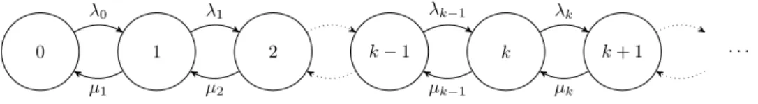
Definition 2.7 (Birth-death process). A birth-death process is a con-tinuous time Markov chain whose states represent the size of a population and whose transitions are limited to unitary births, corresponding to tran-sitions of type k→k+ 1, and unitary deaths, corresponding to transitions of type k→k−1. A birth-death process is fully specified by the birth rates
{λi, i= 0,1, . . .}and the death rates{µi, i= 1,2, . . .}. Its state diagram is
shown in Figure 2.1.
0 1 2 k−1 k k+ 1 · · ·
λ0 λ1 λk−1 λk
µ1 µ2 µk−1 µk
Figure 2.1. State diagram of a birth-death process.
Definition 2.8 (Phase-type distribution). Denote by {X(t), t≥0} an homogeneous Markov process with finite state space SX = {1, . . . , n+ 1},
where we assume that states 1, . . . , n are transient, while state n+ 1 is absorbing. Therefore, the infinitesimal generator matrix of X(t) is of the following form,
(2.6) Q=
T η
0 0
where Tis a square matrix of ordern,η is a column vector of dimension n
called the exit vector, and 0 is the zero row vector of the same dimension. Denoting by1 the column vector of dimensionnwhose entries are all equal to one, we have that η=−T 1. The initial distribution of X(t) is given by
the vector
(2.7) α˜ = (α, αn+1),
where α is a row vector of dimensionn andαn+1= 1−α1.
The random variable T∗, denoting the time until absorption in state
n+ 1, is said to be distributed according to a phase-type distribution of order n with parameters α and T, and we write T∗ ∼ PH(α,T). It can
be proven (see, for example, [10, Ch. 9]) that the cumulative distribution function of T∗ is given by
(2.8) F∗(t) = 1−αeTt1, t≥0,
and that its probability density function is given by
(2.9) f∗(t) =αeTtη, t≥0,
whereeTt=P∞
k=0t
k
k!Tkdenotes the matrix exponential. Moreover, its mo-ments are as follows,
(2.10) E[(T∗)n] = (−1)nn!αT−n1, n∈N. 2.2. Non-homogeneous Poisson processes
Definition 2.9 (Counting process). A stochastic process{N(t), t≥0}
is said to be a counting process if the following conditions hold, for all s, t≥0,
(1) N(t)∈N,
(2) s≤t⇒N(s)≤N(t).
If s < t, thenN(t)−N(s) is the number of events that occurred during the interval (s, t].
Definition 2.10 (Non-homogeneous Poisson process). A counting pro-cess {N(t), t≥0} is said to be a non-homogeneous Poisson process with time-dependent rate λ(t)≥0,t≥0, if the following conditions hold,
(1) N(0) = 0,
(2) {N(t), t≥0}has independent increments, (3) P[N(t+ ∆t)−N(t) = 1] =λ(t) ∆t+o(∆t), (4) P[N(t+ ∆t)−N(t)≥2] =o(∆t),
where o(∆t) is such that
(2.11) lim
∆t→0
o(∆t)
∆t
= 0.
6 2. STOCHASTIC PROCESSES
Theorem2.1. Let{N(t), t≥0}be a non-homogeneous Poisson process with time-dependent rate λ(t). We have that
(2.12) N(t+ ∆t)−N(t)∼Poisson(Λ(t+ ∆t)−Λ(t)) where
(2.13) Λ(t) =
Z t
0
λ(τ)dτ.
Proof. The proof of Theorem 2.1 can be found in classic books on stochastic processes, such as the ones by Ross [39, Ch. 2] and Lefebvre [30, Ch. 5], to which the interested reader is referred.
Corollary 2.1. Let{N(t), t≥0} be a non-homogeneous Poisson pro-cess with time-dependent rateλ(t). It follows immediately from Theorem 2.1 that
(2.14) N(t)∼Poisson(Λ(t)).
2.2.1. Distribution of the first arrival time. We now derive the main result that links the probability distribution of the time of the first ar-rival in a non-homogeneous Poisson process with time-dependent rate λ(t) with this rate function itself. Moreover, we use this result to show the relation between particular forms of λ(t) and well-known probability distri-butions for the time of the first arrival.
Lemma 2.1. Denote by T∗ the random variable representing the time of
the first arrival in a non-homogeneous Poisson process {N(t), t≥0} with time-dependent rateλ(t). The cumulative distribution function ofT∗ at time
t, i.e. the probability that the first arrival occurs before or at time t, can be rewritten in terms of Λ(t) as follows,
(2.15) F∗(t) = 1−e−Λ(t). Its probability density function is thus given by
(2.16) f∗(t) = dF
∗
dt =λ(t)e
−Λ(t).
Proof. The probability that the first arrival occurs before or at time t is equivalent to the probability that at least one arrival occurred during the interval [0, t],
F∗(t) =P[N(t)≥1] = 1−P[N(t) = 0] (2.17)
= 1−e−Λ(t).
Differentiating the previous equation with respect to tyields
(2.18) f∗(t) = dF
∗
dt =λ(t)e
−Λ(t),
Theorem2.2. Given a random variableT whose distribution is given by the cumulative distribution function F(t), t∈R, denote the associated prob-ability density function by f(t), t ∈ R, and define the conditioned random
variable T∗ = T|T ≥ 0. Note that T coincides with T∗ if and only if the
support of its distribution is limited to the interval [0,+∞). The probability density function of T∗ is given by
(2.19) f∗(t) = f(t)
1−F(0), t≥0,
and its cumulative distribution function by
(2.20) F∗(t) =
Z t
0
f∗(τ)dτ = F(t)−F(0)
1−F(0) , t≥0.
The random variable T∗ represents the time of the first arrival in a
non-homogeneous Poisson process with time-dependent rate λ(t) if and only if
(2.21) λ(t) = f
∗(t)
1−F∗(t) =
f(t)
1−F(t), t≥0.
Proof. By Lemma 2.1, we know that the cumulative distribution func-tion of the random variable T∗ is given by
(2.22) F∗(t) = 1−e−Λ(t).
Simple algebraic manipulation immediately yields Equation (2.21), which is
what we wanted to prove.
Corollary 2.2. The time T∗ of the first arrival in a homogeneous Poisson process with fixed rate λ is distributed according to an exponential distribution with parameter λ.
Proof. This is a special case in which (2.23) λ(t) =λ, t≥0. By Theorem 2.2, we only have to prove that
(2.24) f(t)
1−F(t) =λ,
where f(t) and F(t) are the probability density function and the cumula-tive distribution function, respeccumula-tively, of an exponential distribution with parameter λ. In fact, we have that
(2.25) f(t) =λ e−λt and F(t) = 1−e−λt,
from which Equation (2.24) immediately follows.
Definition 2.12 (Weibull distribution). A random variable X is said to be distributed according to a Weibull distribution with shape parameter k∈R,k >0, and scale parameterλ∈R,λ >0, and we writeX∼Ψ(k, λ), if it has probability density function
(2.26) fX(x) =
k λ
x
λ
k−1
8 2. STOCHASTIC PROCESSES
and cumulative distribution function
(2.27) FX(x) =
Z x
0
fX(t)dt= 1−e−(x/λ) k
, x≥0.
Its first moment is given by
(2.28) E[X] =λΓ
1 + 1 k
,
where Γ(z) is the Gamma function.
Corollary 2.3. The time T∗ of the first arrival in a non-homogeneous
Poisson process is distributed according to a Weibull distribution with pa-rameters
(2.29) k=β and λ=
β α
1/β
if and only if the time-dependent rate λ(t) is of the form
(2.30) λ(t) =α tβ−1, t≥0, α, β >0.
Proof. By Theorem 2.2, we only have to prove that
(2.31) f(t)
1−F(t) =α t
β−1,
wheref(t) andF(t) are the probability density function and the cumulative distribution function, respectively, of a Weibull distribution with parameters as per Equation (2.29). In fact, we have that
(2.32) f(t) =α tβ−1e−α tβ/β and F(t) = 1−e−α tβ/β,
from which Equation (2.31) immediately follows.
Definition 2.13 (Gumbel distribution). A random variableXis said to be distributed according to a Gumbel distribution with location parameter µ ∈ R and scale parameter σ ∈ R, σ > 0, and we write X ∼ Λ(µ, σ), if it has probability density function
(2.33) fX(x) =
z e−z
σ , z=e
(x−µ)/σ, x∈R,
and cumulative distribution function
(2.34) FX(x) =
Z x
−∞
fX(t)dt= 1−e−z, x∈R.
Its first moment is given by
(2.35) E[X] =µ−γσ,
where γ ≈0.57722 is the Euler-Mascheroni constant.
to a non-negative Gumbel distribution, and we write X ∼Λ+(µ, σ); it has probability density function
(2.36)
fX+(x) = fX(x) P[X≥0] =
fX(x)
1−FX(0)
= z σe
−z+e−µ/σ
, z=e(x−µ)/σ, x≥0,
and cumulative distribution function
(2.37) FX+(x) =
Z x
0
fX+(t)dt= 1−e−z+e−µ/σ
, z=e(x−µ)/σ, x≥0.
Its first moment is given by
(2.38) EX+=σ ee−µ/σΓ0, e−µσ
,
where Γ(a, z) is the incomplete Gamma function.
Corollary 2.4. The time T∗ of the first arrival in a non-homogeneous
Poisson process is distributed according to a non-negative Gumbel distribu-tion with parameters
(2.39) µ=−1
βln α
β and σ = 1 β
if and only if the time-dependent rate λ(t) is of the form
(2.40) λ(t) =α eβt, t≥0, α, β >0.
Proof. By Theorem 2.2, we only have to prove that
(2.41) f(t)
1−F(t) =α e
βt,
wheref(t) andF(t) are the probability density function and the cumulative distribution function, respectively, of a standard Gumbel distribution with parameters as per Equation (2.39). In fact, we have that
(2.42) f(t) =α e−αeβt/β+βt and F(t) = 1−e−αeβt/β,
Basic concepts from graph theory
In this short presentation we shall only introduce some standard concepts from graph theory, without any pretension of providing a complete account of this vast field of research, for which we refer the interested reader to introductory books such as the one by Diestel [14].
Generally speaking, graphs are composed of a finite set of vertices V
that represent elements of the system being modelled, and a binary relation E ⊆ V2that represents edges, i.e. pairwise interactions between the vertices. While it is possible to consider edges that link a vertexi∈ V to itself, called self-loops, in what follows we shall only be concerned with graphs without self-loops; more formally, this is equivalent to requiring that the binary relation E is irreflexive, (i, i)6∈E for all i∈ V.
3.1. Graphs
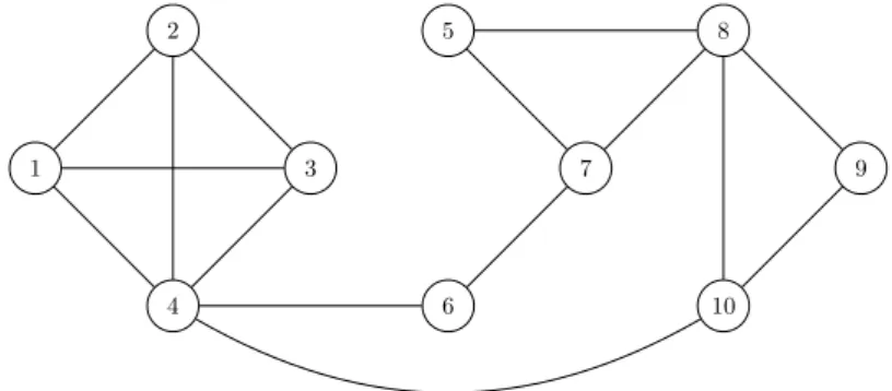
The simplest kind of graph that we shall consider are those in which relations between elements of the system are symmetric. An example is shown in Figure 3.1.
1
2
3
4
5
6
7
8
9
10
Figure 3.1. Example of graph with n = 10 vertices and m= 15 edges.
Definition3.1 (Graph). A graph is a couple (V, E), whereV ={1,2, . . . , n}
is a finite set of vertices (or nodes), and E⊆ V2 is a binary relation over it describing the edges and satisfying, for all i, j∈ V,
(i, i)6∈E (irreflexivity) (3.1a)
(i, j)∈E ⇒(j, i)∈E (symmetry) (3.1b)
12 3. BASIC CONCEPTS FROM GRAPH THEORY
We shall now introduce some useful terminology regarding basic charac-teristics of a graph, such as the number of vertices or edges it contains.
Definition 3.2 (Adjacent vertices or neighbours). Two verticesi, j ∈ V
linked by an edge, (i, j)∈E, are said to be adjacent or neighbours.
For example, vertices 1 and 2 in Figure 3.1 are adjacent or neighbours.
Definition 3.3 (Order of a graph). The order of a graph, commonly denoted n, is the number of its vertices, i.e. the cardinality of the setV.
For example, the graph of Figure 3.1 is of order 10.
Definition 3.4 (Size of a graph). The size of a graph, commonly de-noted m, is the number of its edges. Since edges are commonly defined as the pairs {(i, j),(j, i)}, this number corresponds to half the cardinality of the binary relation E.
For example, the graph of Figure 3.1 is of size 15.
Remark3.1 (Maximum size). The sizemof a graph is clearly connected to its ordern. Because of the irreflexivity requirement, the maximum cardi-nality ofE isn(n−1); this situation corresponds to the complete graph, in which each vertex is connected to all others. Therefore, the maximum size of a graph of order nismmax=n(n−1)/2.
Definition 3.5 (Adjacency matrix). The binary relation E can be ex-plicitly represented by a square symmetric matrixA=AT of ordern, called adjacency matrix, with elements
(3.2) aij =
(
1 if (i, j)∈E
0 otherwise for all i, j∈ V.
Definition 3.6 (Vertex degree). The degree ki of a vertex i ∈ V is
defined as the number of its neighbours. From the point of view of the binary relationE, this corresponds to the cardinality of the subset ofE containing only tuples whose first element is i, or equivalently to the cardinality of the subset of E containing only tuples whose second element is i. In terms of the adjacency matrix A we have that
(3.3) ki =
X
j6=i
aij =
X
j6=i
aji.
For example, vertex 1 in Figure 3.1 has degree 3.
Definition 3.7 (Degree distribution). Given a graph, letpkbe the
frac-tion of its vertices that have degreek. The sequence{pk:k= 0, . . . , n−1}
For example, the degree distribution of the graph shown in Figure 3.1 is
{0,0,0.3,0.5,0.1,0.1,0,0,0}, since it has no vertex with degree zero or one, three vertices with degree two, five vertices with degree three, one vertex with degree four, one vertex with degree five, and no other vertex with higher degree.
Remark3.2. Naturally, the degree distribution does not fully determine the structure of the graph. Typically, there is a significant number of graphs sharing the same degree distribution.
3.1.1. Weighted graphs. A simple extension of graphs consists in associating to each edge a non-negative weight that is usually assumed to represent the strength of the relation; an alternative definition requires that weights belong to the [0,1] interval, an assumption which can always be satisfied by an appropriate rescaling of the values.
It is particularly easy to think of weighted graphs in terms of their ad-jacency matrix representation. In this case, instead of the boolean matrices of simple graphs, we consider adjacency matrices whose elements can take any non-negative real value,
(3.4) aij =aji ≥0 for all i, j∈ V, i6=j.
Definition 3.8 (Adjacent vertices or neighbours). Two verticesi, j ∈ V
are said to be adjacent or neighbours if aij >0.
Definition 3.9 (Vertex degree). The degreeki of a vertexi∈ V is again
defined as the number of its neighbours,
(3.5) ki=
X
j6=i
H(aij) =
X
j6=i
H(aji),
where H(x) is the Heaviside step function whose value is one forx >0 and zero otherwise.
Definition 3.10 (Vertex strength). The strengthsi of a vertexi∈ V is
defined as the sum of the weights of all edges that link it to other vertices,
(3.6) si=
X
j6=i
aij =
X
j6=i
aji.
Note that, in general, the degree ki of a vertexi∈ V is not the same as its
strength si.
3.2. Digraphs
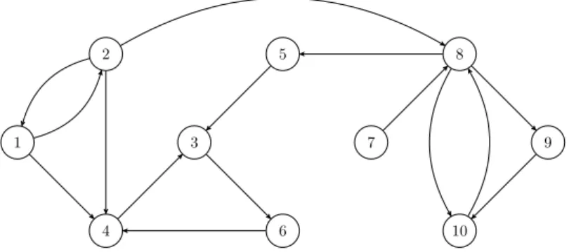
Definition 3.11 (Digraph). Digraphs (from “directed graphs”) are ob-tained by relaxing the symmetry requirement of Definition 3.1, thus allowing each edge to have a direction, commonly represented by an arrow as in Fig-ure 3.2. In this case, the adjacency matrix A is also asymmetric.
14 3. BASIC CONCEPTS FROM GRAPH THEORY
1
2
3
4
5
6
7
8
9
10
Figure 3.2. Example of digraph with n= 10 vertices and m= 15 edges.
For example, vertices 1 and 2 in Figure 3.2 are adjacent or neighbours, and so are 1 and 4. Definition 3.3 also applies to the order of a digraph; its size, however, needs to be redefined as follows.
Definition 3.13 (Size of a digraph). The size of a digraph, commonly denoted m, is the number of its edges, which corresponds to the cardinality of the binary relation E.
Remark 3.3 (Maximum size). Because of the irreflexivity requirement, the maximum cardinality of E is n(n−1); therefore, the maximum size of a digraph of order nismmax=n(n−1).
Moreover, in digraphs it is not possible to define the degree as we did in Definition 3.6, because the number of edges pointing to a vertex i ∈ V
is generally different from the number of edges pointing from i to other vertices.
Definition 3.14 (Vertex in-degree and out-degree). The in-degree kin
i
of a vertex i ∈ V is defined as the number of incoming edges, i.e. edges that start at one of the neighbours of iand end ati; in terms of the binary relationE, this corresponds to the cardinality of the subset ofE containing only tuples whose second element is i. Similarly, the out-degree kiout of the same vertex i is defined as the number of outgoing edges, i.e. edges that start at iand end at one of its neighbours; in terms of the binary relation E, this corresponds to the cardinality of the subset of E containing only tuples whose first element isi. As regards the adjacency matrixA, we have that
(3.7) kiin=X
j
aji and kiout =
X
j
aij.
3.2.1. Weighted digraphs. As for graphs, digraphs can also be ex-tended to include non-negative weights associated to each edge. In this case, the adjacency matrixAis not only asymmetric, but its elementsaij can take
any non-negative real value, aij ≥0 for alli, j∈ V,i6=j.
Definition 3.15 (Adjacent vertices or neighbours). Two verticesi, j ∈ V are said to be adjacent or neighbours if aij >0 or aji>0.
Definition 3.16 (Vertex in-degree and out-degree). The in-degree kini and the out-degree kout
i of a vertexi ∈ V are again defined as the number
of incoming and outgoing edges, respectively,
(3.8) kini =X
j
H(aji) and kiout =
X
j
H(aij) ,
where H(x) is the Heaviside step function whose value is one forx >0 and zero otherwise.
Mathematical epidemiology of infectious diseases
4.1. Modelling assumptions
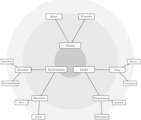
Many mathematical models for the spread of infectious diseases have been proposed in the literature, and it is often too easy to get lost in their details. Since models necessarily encompass a set of assumptions, it makes sense to classify them according to the hypotheses they are based on [13, Ch. 1]. As shown in Figure 4.1, assumptions roughly belong to three main categories, namely:
(1) assumptions about the disease itself;
(2) assumptions about the environment within which the disease spreads; (3) assumptions due to mathematical modelling.
Assumptions about the disease mostly regard the possible states (also sometimes called compartments) according to which individuals are exclu-sively and exhaustively classified at any given time, and dynamics among them. In this work we shall restrict ourselves to contagious illnesses, under the basic assumption that diseases spread as a result of contacts between susceptible and infective (carrier) individuals1. In this context, models range from the simplest S →I model, in which individuals are either susceptible to the disease (S) or forever infected with it (I), to more complex extensions that account for different stages of infection (such as incubation periods), temporary recovery, removals (which may themselves be due to different causes, such as acquired immunity, isolation, or death), vaccinations and vertical transmission and immunity. Of course, realistic assumptions about the disease can only be formulated based on the epidemiological properties of the pathogen. However, the time scale being considered also plays a cru-cial role: in the case of influenza, for example, it is reasonable and often easier to assume that, in a single season, an individual can only catch the disease once, and thus earns “lifelong” immunity after the infection.
Assumptions regarding the environment can be further classified into two subcategories: assumptions about its structure and about its dynamics. As for structure, an important distinction needs to be made between pop-ulation models, which deal with a single poppop-ulation, and meta-poppop-ulation
1Note that this assumption does indeed exclude a number of diseases, for example
those that spread through intermediate vector species (such as mosquito for malaria and yellow fever). It is of course possible to model these illnesses as well, and one of the landmarks in the development of mathematical epidemiology is indeed the work of Ross [38] on malaria.
18 4. MATHEMATICAL EPIDEMIOLOGY OF INFECTIOUS DISEASES
Environment Disease
Model Structure
Dynamics
States Dynamics
Formulation Time
Population
Meta-population
Open
Closed Deterministic
Stochastic Continuous
Discrete
Figure 4.1. Categorization of assumptions in epidemiolog-ical models of infectious diseases: the three main categories include assumptions about the disease itself, the environment within which it spreads, and the mathematical model itself.
models, which consider a set of populations and constrained interactions among them, such as travel of individuals. The population (or populations, in the case of meta-population models) may be considered as a single, ho-mogeneous group, as a collection of several hoho-mogeneous strata, or else as completely heterogeneous. In all cases it is also necessary to define the population dynamics, which range from closed populations, with a constant number of individuals, to open populations considering complex birth and death processes, as well as migrations.
intervals can be made as small as desired, continuous time models can be considered as limiting cases, and usually offer interesting insights as well as better analytical tractability.
As said, the choice between deterministic and stochastic models is far more important than the one between discrete or continuous time, which can be made to correspond in the case of infinitesimal time increments. His-torically, it is interesting to note that the development of deterministic and stochastic models has occurred almost in parallel. However, it is crucial to understand that the spread of infectious diseases is intrinsically a stochastic process: the same initial conditions may lead to very different outcomes, from small outbreaks to large-scale epidemics. It follows that any determin-istic model that evolves according to fixed rules, depending only on initial parameter values, is at best an approximation of the actual process.
The effects of stochasticity are particularly relevant in the case of small populations [13, Ch. 3]. Even for larger populations, at the beginning of most outbreaks the number of infective individuals is usually small, so that the population might not mix homogeneously, making transmission of the disease depend strongly on the pattern of contacts [8].
As for the actual mathematical tools used, stochastic models are usually formulated as stochastic processes over a set of random variables represent-ing the number of individuals in each state; their solutions are thus probabil-ity distributions for each random variable. On the other hand, deterministic models are often formulated as systems of differential or difference equations; their solutions are functions of discrete or continuous time that indicate the fraction of population in each state.
4.2. Deterministic models
4.2.1. The S →I model. The simplest epidemic model, due to Ross [38], contemplates only two states, the susceptible (S) and infective (I), and assumes that the disease spreads in a single closed population and that indi-viduals mix homogeneously, so that each one has equal chance of becoming infective. Because of this last assumption, we can apply the law of mass ac-tion2 and thus consider that the rate of interaction between the two sets of susceptible and infective individuals is proportional to the product of their cardinalities.
Let us denote by S(t) and I(t) the number of susceptible and infective individuals at time t, respectively, and by s(t) and i(t) the corresponding fractions of the population,
(4.1) s(t) =S(t)
N and i(t) = I(t)
N ,
since the population size is assumed constant and equal to N. Taking into account the law of mass action, the S → I model can be schematized as 2This chemical law, due to Waage and Guldberg [42], states that, in a homogenous
20 4. MATHEMATICAL EPIDEMIOLOGY OF INFECTIOUS DISEASES
follows,
(4.2) S −→β I,
and formulated as the following system of non-linear ordinary differential equations,
dS
dt =−β S(t)I(t) , (4.3a)
dI
dt =β S(t)I(t) , (4.3b)
together with suitable initial conditions for the number of susceptible and infective individuals at time t= 0,
S(0) = (1−α)N, (4.4a)
I(0) =α N, (4.4b)
where 0≤α≤1 is the fraction of population that is initially infective,β >0 represents the per capita transmission rate, and clearlyS(0) +I(0) =N as required.
Since the population size is assumed constant, we have that S(t) = N−I(t) at all timet >0, which in turn means that the previous system has only one degree of freedom, and can be equivalently expressed by a single differential equation,
(4.5) dI
dt =β I(t) (N −I(t)) .
This equation can be explicitly solved by separation of variables, yielding
(4.6) I(t) = I(0)N
I(0) + (N−I(0))e−βN t,
from which it can be easily seen that, eventually, all individuals become infective,
(4.7) lim
t→+∞I(t) =
I(0)N I(0) =N.
Assuming that I(0) = α N, 0 ≤α ≤1 as per Equation (4.4b) and substi-tuting in the equation above gives
(4.8) I(t) = α N
α+ (1−α)e−βN t.
0 0.2 0.4 0.6 0.8 1
0 50 100 150 200 250 300 350 400 450 500
i
(
t
)
t
β= 5×10⁻⁸ β= 1×10⁻⁷ β= 2×10⁻⁷
Figure 4.2. Evolution of the infective fraction of population in the deterministicS →Imodel for different values ofβ; the population is of sizeN = 106 and initially a single individual is infective (α=N−1).
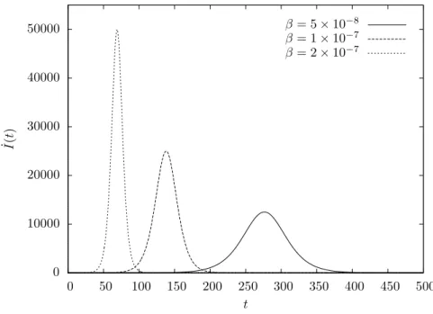
4.2.1.1. Epidemic curve. Another interesting function that can be im-mediately derived from Equation (4.8) is the epidemic curve ˙I(t) that repre-sents the rate of change of I(t). This function is of particular interest since real-world data is usually made available in this form, i.e. as the number of new infective individuals over time. This means that model parameters could in principle be inferred by adjusting an epidemic curve to available data; however, the sparseness and inaccuracy that characterizes this infor-mation makes it very difficult to do so, which is why we consider a different approach in Chapter 6.
Differentiating Equation (4.8) yields
(4.9) I˙(t) = dI dt =
α(1−α)β N2eβN t (α(eβN t−1) + 1)2,
some graphs of which are shown in Figure 4.3. This function is symmet-ric and unimodal; its maximum can be determined as the solution to the following equation,
(4.10) dI˙ dt =
α(α−1)β2N3eβN t α+αeβN t−1
(α(eβN t−1) + 1)3 = 0,
which gives
(4.11) tmax= 1 βN ln
1−α
α and I˙(tmax) = βN2
22 4. MATHEMATICAL EPIDEMIOLOGY OF INFECTIOUS DISEASES
Furthermore, since
(4.12) lim
N→+∞tmax= 0,
we note that, the larger the population, the sooner ˙I(t) attains its maximum, as we would expect.
0 10000 20000 30000 40000 50000
0 50 100 150 200 250 300 350 400 450 500
˙I(t
)
t
β= 5×10⁻⁸ β= 1×10⁻⁷ β= 2×10⁻⁷
Figure 4.3. Epidemic curve in the deterministic S → I model for different values ofβ; the population is of sizeN = 106 and initially a single individual is infective (α=N−1).
4.2.2. The S → I → R model. A more complex epidemic model, due to Kermack and McKendrick [27, 28, 29], builds on the simpler S →I introduced in the previous section by considering a third state, the removed (R), which encompasses all infective individuals that no longer contribute to the spreading process and that cannot be reinfected. The rate of removal is assumed to be proportional to the number of infective individuals.
Given the above assumption, the S → I → R model can be easily schematized as follows,
(4.13) S−→β I −→γ R,
and formulated as the following system of non-linear ordinary differential equations,
dS
dt =−β S(t)I(t), (4.14a)
dI
dt =β S(t)I(t)−γ I(t), (4.14b)
dR
where the parameterγ represents the instantaneous recovery rate, so that its reciprocalγ−1 represents the expected duration of the infectious period. In addition to specifying suitable initial conditions for the number of susceptible and infective individuals at time t = 0, one also needs to do so for the number of removed individuals R(0) that, when greater than zero, can be interpreted as that part of the population that is initially immune to the disease. Similarly to theS →I model, since the population size is assumed constant, the previous system has only two degrees of freedom, and can be equivalently expressed by any two of the three differential equations together with the condition S(t) +I(t) +R(t) =N at all timet >0.
Despite being straightforward to formulate, the S→I →R model can-not be solved analytically; as we shall see, however, a number of interesting properties can nonetheless be derived from analytical considerations.
4.2.2.1. The basic reproduction number R0. Suppose that all individuals in a population are initially susceptible, and that one of them becomes infective. This individual can be expected to infect the S(0) susceptible individuals at a rateβ during the expected infectious period γ−1; therefore, the total expected number of secondary cases it causes is given by
(4.15) R0 =
β S(0)
γ ≈
β N γ ,
which is commonly known as the basic reproduction number. The number R0 is of paramount importance in epidemic modelling: in particular, it determines whether an epidemic can occur at all3. Intuitively, since R0 represents the expected number of secondary cases caused by introduction of a single infective individual into a completely susceptible population, no epidemic can develop if this number is smaller than one, since in this case the number of infective individuals in each successive generation decreases with time.
Theorem 4.1 (Kermack-McKendrick Threshold Theorem). A major outbreak occurs if and only if the rate of change at t = 0 of the number of infective individuals I(0) is strictly positive; this happens if and only if
R0 >1.
Proof. From Equation (4.14b), we have that the rate of change of the number of infective individuals I(t) is strictly positive if and only if
(4.16) β S(t)I(t)−γ I(t)>0 or S(t)> γ β.
Therefore, I(t) increases as long as S(t) > γ/β; however, since S(t) is a decreasing function of t, I(t) must also ultimately decrease and approach zero. More specifically, if S(0) < γ/β, which corresponds to the condition
3The threshold behaviour that theS →I→Rmodel exhibits is not only consistent
24 4. MATHEMATICAL EPIDEMIOLOGY OF INFECTIOUS DISEASES
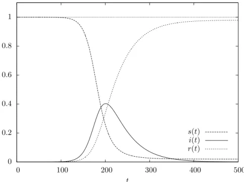
R0 <1, it does so immediately, and no epidemic takes place; otherwise, the so-calledepidemic regime occurs: the functionI(t) first attains a maximum, when S(t) =γ/β, and then decreases to zero.
Figure 4.4 shows the evolution over time of the fractions of population in each of the three states in this second case.
0 0.2 0.4 0.6 0.8 1
0 100 200 300 400 500
t
s(t)
i(t)
r(t)
Figure 4.4. Evolution of the fractions of population in the three different states in the epidemic regime of the determin-istic S → I → R model with β = 10−7, γ = 0.025, and a population of size N = 106, thus yieldingR
0 = 4; initially a single individual is infective (α =N−1), while all others are susceptible.
4.2.2.2. Epidemic curve. As for theS→I model, it is possible to derive an expression for the epidemic curve associated with theS →I →Rmodel. However, instead of defining it as the rate of change of the number of infective individuals I(t), as we did in Section 4.2.1.1, we shall consider the rate of change of the number of removed individuals R(t). This definition is realistic if we assume that infective individuals are immediately removed when symptoms are detected, for example because they are quarantined or isolated to undergo treatment.
Dividing Equation (4.14a) by Equation (4.14c), we get the differential equation
(4.17) dS
dR =
−β S(t)I(t) γ I(t) =−
that can be easily integrated (assuming R(0) = 0), yielding
(4.18) S(t) =S(0)e−β R(t)/γ,
which, substituted into Equation (4.14c), gives
(4.19) dR
dt =γ I(t) =γ(N−S(t)−R(t)) =γ
N −S(0)e−βγR(t)−R(t)
.
Considering now the quadratic Taylor polynomial approximation for the exponential term,
(4.20) e−βγR(t)≈1− β
γR(t) + β2 2γ2R
2(t),
we obtain the following approximation for Equation (4.14c),
dR dt ≈γ
N −S(0)
1−β
γR(t) + β2 2γ2R
2(t)
−R(t)
=γ
β2S(0) 2γ2 R
2(t) +
β S(0) γ −1
R(t) +N −S(0)
(4.21)
=γ
R20 2S(0)R
2(t) + (R
0−1)R(t) +N −S(0)
,
which can be explicitly solved by separation of variables (again assuming R(0) = 0), giving
(4.22) R(t)≈ γ
β R0
R0−1 +φtanh
γ φ 2 t−ψ
,
where we have defined
φ=
s
(R0−1)2− 2β2
γ2 S(0)I(0), (4.23a)
ψ= arctanh
R0−1 φ
. (4.23b)
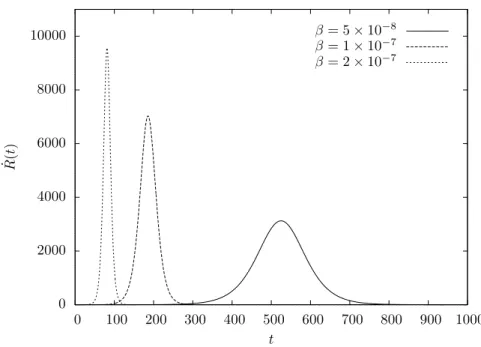
By differentiation of Equation (4.22), we can obtain an approximate expres-sion for the epidemic curve,
(4.24) R˙(t)≈ γ
3φ2
2β2S(0)sech 2
γ φ 2 t−ψ
,
some graphs of which are shown in Figure 4.5.
26 4. MATHEMATICAL EPIDEMIOLOGY OF INFECTIOUS DISEASES 0 2000 4000 6000 8000 10000
0 100 200 300 400 500 600 700 800 900 1000
˙R(t
)
t
β= 5×10⁻⁸
β= 1×10⁻⁷
β= 2×10⁻⁷
Figure 4.5. Epidemic curve in the deterministic S → I →
R model for different values of β and γ = 0.025; the popu-lation is of size N = 106 and initially a single individual is infective (α=N−1).
Theorem 4.2 (Kermack-McKendrick Survival Theorem). Let us intro-duce the following notation,
(4.25) S∞= lim
t→∞S(t), I∞= limt→∞I(t), R∞= limt→∞R(t).
When the disease ultimately ceases spreading, a positive number S∞>0 of
susceptible individuals remain uninfected.
Proof. Since S(t) +I(t) +R(t) = N at all time t > 0, we have that R(t)≤N at the same time. Therefore, from Equation 4.18 we have that (4.26) S∞=S(0)e−β R∞/γ ≥S(0)e−β N/γ,
which shows that S∞>0.
An equation forS∞can be obtained as follows. Dividing Equation (4.14b)
by Equation (4.14a), we get the differential equation
(4.27) dI
dS =
β S(t)I(t)−γ I(t)
−β S(t)I(t) =−1 + γ β S(t),
which can be easily integrated, taking into account the initial conditions S(0) and I(0), yielding
(4.28) S(t) +I(t)− γ
β lnS(t) =S(0) +I(0)− γ
βlnS(0). Taking the limit as t→ ∞ and rearranging the terms leads to
(4.29) S∞=N−
γ β ln S(0) S∞ ≈N
1− 1
R0
lnS(0) S∞
where we have assumed that R(0) = 0, so that S(0) +I(0) = N, and we have made use of Equation 4.15 and of the fact that I∞= 0.
4.2.3. Other models. TheS →I and S→I →Rmodels introduced above are the most simple compartmental models, but are nonetheless cru-cial as building blocks of more complex models: the S →I →R model, for example, is already an extension of the simpler S → I model (to see this, consider the case γ = 0).
Possible extensions include new states, as in the S → E → I → R model that allows for “exposed” individuals (E), i.e. individuals in which the disease is latent and manifests itself at a constant rate, as well as the possibility of reinfection, as in the S → I → R → S, in which removed individuals regain susceptibility at a constant rate. All these models can be further extended by considering population dynamics (births and deaths, which are commonly considered to occur at the same rate to keep the total population size N constant), and vaccination strategies.
4.3. Stochastic models
In this section we shall introduce, following the presentations of Daley and Gani [13] and Allen [2], some stochastic models in discrete and contin-uous time that have been proposed in the literature.
As a general remark, it is important to note that, whereas stochastic models have a natural deterministic description that can be obtained by taking expected values of the involved quantities, the reverse does not hold true: starting with a system of differential equations, one can derive a variety of corresponding stochastic models whose deterministic skeleton corresponds to the starting system of differential equations [24].
4.3.1. Chain binomial models. Chain binomial models are among the first discrete time stochastic epidemic models that were studied; as their name implies, they entail sequences of binomially distributed random vari-ables. There are two classic such models: one is due to Reed and Frost and was put forward in their lectures at Johns Hopkins University in 1928, but never published, until Abbey [1] gave a detailed account of it; the other is due to Greenwood [23]. They are both Markov chains, even though this fact was not fully appreciated until the work of Gani and Jerwood [20].
28 4. MATHEMATICAL EPIDEMIOLOGY OF INFECTIOUS DISEASES
are simultaneously in the infectious period (as is necessarily the case with a single initially infective individual), the disease will spread in successive generations that do not overlap in time. This characteristic sets this model radically apart from the S → I → R model of Section 4.2.2, whose great applicability to real-world data may well be due to the possibility of smaller scale overlapping epidemics [13].
Consider the two random variables St and It with discrete state spaces SS =SI ={0,1, . . . N}representing the number of susceptible and infective
individuals at time t, respectively. Note that St+It=St−1. Let us denote by p ∈(0,1) the probability of contact between a susceptible and an infec-tive individual, and by β∈(0,1) the probability that this contact results in infection of the susceptible individual by the infective one. Then, the prob-ability αthat there is no infection due to any single infective individual can be expressed as the sum of two probabilities: (a) the probability (1−p) that no contact with an infective individual occurs; (b) the probabilityp(1−β) that a contact with an infective individual occurs, but that this contact does not result in infection. Thus, we have that
(4.30) α= (1−p) +p(1−β) = 1−p β.
The Greenwood model [23] assumes that the cause of infection is unre-lated to the number of infective individuals, so that α is simply the proba-bility of non-infection. In this case, we have that It=St−1−St, and
P[St+1 =st+1, It+1 =it+1|St=st, It=it]
=
st
st+1
αst+1(1−α)it+1=
st
st+1
αst+1(1−α)st+1−st, (4.31)
which shows that {St, t= 0,1, . . .} is a univariate Markov chain, since It
fully depends on St, and the value of the latter at time t+ 1 depends only
on its value at time t.
The Reed-Frost model [1], on the other hand, considers that a suscep-tible individual remains so from t to t+ 1 only if infectious contact with all It infective individuals is avoided, which occurs independently for each
susceptible individual with probability αIt. Thus St+1 ∼Binomial St, αIt,
and
P[St+1=st+1, It+1 =it+1|St=st, It=it]
=
st
st+1
αitst+1 1−αitit+1, (4.32)
which shows that {(St, It), t= 0,1, . . .} is a bivariate Markov chain, since
the values of St and It at timet+ 1 depend only on their values at time t.
Since the numbers of infective individuals in successive generations are binomially distributed, it is possible to readily compute their expectations. For the Greenwood model, Equation (4.31) immediately yields
and thus
E[St|S0=s0] =αts0, (4.34a)
E[It|S0=s0] =αt−1(1−α)s0. (4.34b)
It follows from Equation (4.34a) that E[St] → 0 as t → ∞, which means that, since Stis non-negative, it holds thatSt= 0 for all sufficiently larget.
As for the Reed-Frost model, Equation (4.32) yields
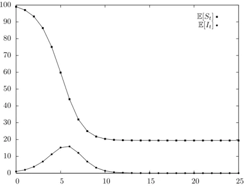
(4.35) E[St+1, It+1|St=st, It=it] = stαit, st 1−αit.
These equations, unlike those we determined for the Greenwood model, do not lead to an explicit solution; however, given their recurrent nature, they can be easily evaluated numerically, as shown in Figure 4.6.
0 10 20 30 40 50 60 70 80 90 100
0 5 10 15 20 25
E[St] E[It]
Figure 4.6. Evolution of the expected number of suscep-tible and infective individuals in the Reed-Frost model; the probability of no infection is α = 0.98, the population is of sizeN = 100, and initially a single individual is infective.
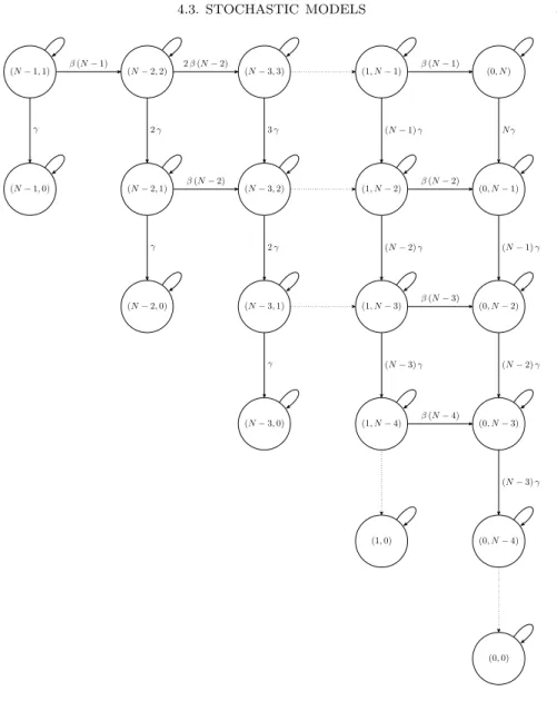
4.3.2. Continuous time Markov chain. We now move to continuous time Markov chains, which are a natural way to introduce stochasticity into the deterministic S→I →R model of Section 4.2.
Consider the two random variables S(t) and I(t) with discrete state spaces SS = SI ={0,1, . . . N} representing the number of susceptible and
30 4. MATHEMATICAL EPIDEMIOLOGY OF INFECTIOUS DISEASES
We can thus define the bivariate Markov process {(S(t), I(t)), t≥0}
with infinitesimal transition probabilities as follows,
P[S(t+ ∆t) =s+ ∆S, I(t+ ∆t) =i+ ∆I|S(t) =s, I(t) =i]
=
β s i∆t+o(∆t) ∆S =−1,∆I = 1,
γ i∆t+o(∆t) ∆S = 0,∆I =−1,
1−(β s+γ)i∆t+o(∆t) ∆S = 0,∆I = 0,
o(∆t) otherwise,
(4.36)
where o(∆t) is such that
(4.37) lim
∆t→0
o(∆t)
∆t
= 0,
and we again assumed that ∆t is sufficiently small that at most a single
transition (either S+I → 2I or I → R) occurs. The possible states and transitions among them are schematized in Figure 4.7.
Writing the state probabilities as follows,
(4.38) p(s,i)(t) =P[S(t) =s, I(t) =i|S(0) =s0, I(0) =i0],
where s0 ∈ SS, i0 ∈ SI are the initial number of susceptible and infective
individuals, respectively, and s0+i0 ≤N, we have that
p(s0,i0)(t+ ∆t) = [1−(β s0+γ)i0∆t]p(s0,i0)(t) +o(∆t), (4.39a)
p(s,i)(t+ ∆t) =β(s+ 1) (i−1) ∆tp(s+1,i−1)(t) +γ(i+ 1) ∆tp(s,i+1)(t)
(4.39b)
+ [1−(β s+γ)i∆t]p(s,i)(t) +o(∆t),
since, as shown in Figure 4.8, the probability of being in state (s, i) at time t+ ∆t can be written by the Markov property as the sum of: (a) the
probability of being in state (s+ 1, i−1) at time t and that the transition that occurred wasS+I →2I; (b) the probability of being in state (s, i+ 1) at timetand that the transition that occurred wasI →R; (c) the probability of being in state (s, i) at timet and that no transition occurred.
Subtracting p(s0,i0)(t) on both sides of Equation (4.39a) andp(s,i)(t) on both sides of Equation (4.39b), dividing by ∆tand taking the limit as ∆t→0
leads to the following system of forward Kolmogorov differential equations,
dp(s0,i0)
dt =−(β s0+γ)i0p(s0,i0)(t), (4.40a)
dp(s,i)
dt =β(s+ 1) (i−1)p(s+1,i−1)(t) +γ(i+ 1)p(s,i+1)(t)
(4.40b)
−(β s+γ)i p(s,i)(t),
(N−1,1) (N−2,2) (N−3,3) (1, N−1) (0, N)
(N−1,0) (N−2,1) (N−3,2) (1, N−2) (0, N−1)
(N−2,0) (N−3,1) (1, N−3) (0, N−2)
(N−3,0) (1, N−4) (0, N−3)
(1,0) (0, N−4)
(0,0)
β(N−1)
γ
2β(N−2)
2γ 3γ
β(N−1)
(N−1)γ N γ
γ
β(N−2)
2γ
β(N−2)
(N−2)γ (N−1)γ
γ
β(N−3)
(N−3)γ (N−2)γ
β(N−4)
(N−3)γ
Figure 4.7. Bivariate Markov chain S → I → R model: each state in the chain is characterized by a couple (S, I) representing the number of susceptible individualsSand that of infective individuals I; the initial state depends on the initial conditions, but is usually assumed to be (N −1,1); note that all states with I = 0 are absorbing.
We next present a threshold theorem, similar to Theorem 4.1, for the stochastic S →I →R model.
Theorem 4.3 (Whittle’s Threshold Theorem). For any α ∈ (0,1), let
32 4. MATHEMATICAL EPIDEMIOLOGY OF INFECTIOUS DISEASES
(s, i) (s+ 1, i−1)
(s, i+ 1)
S+I→2I
I→R
Figure 4.8. Possible transitions in the bivariate Markov chain S → I → R model during the infinitesimal time in-terval (t, t+ ∆t).
holds that
if R0≤1, then π(α) = 1, (4.41a)
if 1< R0≤ 1
1−α, then
1 R0
I(0)
≤π(α)≤1,
(4.41b)
if R0> 1
1−α, then
1 R0
I(0)
≤π(α)≤
1 (1−α)R0
I(0)
.
(4.41c)
Proof. The proof of Theorem 4.3 can be found, for example, in [13, Ch. 3]; the original result is due to Whittle [43]. The basic idea behind the proof is to bound the componentI(t) between two birth-death processes.
Remark4.1. ForR0 ≤1, we have that the probability that the epidemic achieves an intensity greater than any α ∈ (0,1) is zero. This result is strikingly similar to that of Theorem 4.1 for the deterministic S → I → R model, which predicted that no epidemic would occur for R0 ≤1.