Quality control in clothing manufacturing with machine learning

(1)

University Institute of Lisbon

Department of Information Science and Technology

Quality Control in Clothing

Manufacturing with Machine

Learning

Gonçalo Laginha Serafim San-Payo

Dissertation submitted as partial fulfillment of the requirements for

the degree of

Master in Computer Engineering

Supervisor

PhD João Carlos Amaro Ferreira, Assistant Professor

ISCTE-IUL

Co-Supervisor

PhD João Pedro Afonso Oliveira da Silva, Assistant Professor

ISCTE-IUL

(2)

(3)

Resumo

O controlo de qualidade é vital para um negócio e a aprendizagem automática tem provado ser bem-sucedida neste tipo de área. Neste trabalho propomos e desenvolvemos um sistema de controlo de qualidade para o fabrico de roupas uti-lizando aprendizagem automática. O sistema consiste em usar fotografias, tiradas através de dispositivos móveis, para detetar defeitos em peças de roupa. Um de-feito pode ser a falta de um componente ou um componente errado numa peça de roupa. A função do sistema é, portanto, classificar os objetos que compõem uma peça de roupa através do uso de um modelo de classificação. À medida que um negócio fabril progride, novos objetos são criados, assim, o modelo de classificação deve ser capaz de aprender as novas classes sem perder conhecimento prévio. No entanto, a maioria dos algoritmos de classificação não suporta um aumento de classes, estes precisam ser treinados a partir do zero com todas as classes. Neste trabalho, utilizamos um algoritmo que suporta aprendizagem incremental para re-solver este problema. Este algoritmo classifica características extraídas de imagens das peças de roupa usando uma rede neural convolucional, que tem provado ser uma técnica muito bem sucedida no que toca a resolver problemas de classificação de imagem. Como resultado deste trabalho, desenvolvemos um sistema de controlo de qualidade que combina uma aplicação móvel para tirar fotografias de peças de roupa e um servidor que executa os processos de deteção de defeitos usando um modelo de classificação de imagens preciso, capaz de aumentar o seu conhecimento a partir de novos dados nunca antes vistos. Este sistema pode ajudar as fábricas a melhorar seus processos de controlo de qualidade.

Palavras-chave: Controlo de qualidade, aprendizagem incremental,

(4)

(5)

Abstract

Quality control is vital for business and machine learning has proven to be successful in this type of area. In this work we propose and develop a classifica-tion model to be used in a quality control system for clothing manufacturing using machine learning. The system consists of using pictures taken through mobile devices to detect defects on clothing items. A defect can be a missing component or a wrong component in a clothing item. Therefore, the function of system is to classify the objects that compose a clothing item through the use of a classification model. As a manufacturing business progresses, new objects are created, thus, the classification model must be able to learn the new classes without losing previous knowledge. However, most classification algorithms do not support an increase of classes, these need to be trained from scratch with all classes. In this work, we make use of an incremental learning algorithm to tackle this problem. This algorithm classifies features extracted from pictures of the clothing items using a convolutional neural network (CNN), which have proven to be very successfully in image classification problems. As the result of this work, we have developed a quality control system that combines a mobile application to take pictures of cloth-ing items and a server that performs defect detection processes uscloth-ing an accurate image classification model capable of increasing its knowledge from new unseen data. This system can help factories improve their quality control processes.

(6)

(7)

Acknowledgements

I would like to acknowledge my supervisors, Professors João Ferreira and João Oliveira, for their guidance and support. To all the people at INOV INESC Ino-vação for providing me a great work environment as well as the tools to develop this work.

A special thanks to my parents, Margarida and Miguel, for motivating me to achieved greater goals.

And last, but not least, to my closest friends that shared long nights of writing with me. Without them this thesis would not be finished on time.

(8)

(9)

Resumo iii Abstract v Acknowledgements vii List of Figures xi Abbreviations xiv 1 Introduction 1 1.1 Overview . . . 1 1.2 Motivation . . . 2 1.3 Objectives . . . 3 1.4 Document Structure . . . 4 2 Literature Review 7 2.1 Image Classification . . . 7 2.1.1 Deep Learning . . . 8 2.1.1.1 Transfer Learning . . . 12 2.1.1.2 Libraries . . . 14 2.1.2 Data Augmentation . . . 14 2.2 Incremental Learning . . . 15 2.3 Quality Control . . . 18

3 Quality Control System for Clothing Manufacturing 21 3.1 Defect Detection Server . . . 25

3.1.1 Image Database . . . 26

3.1.2 Defect Registration . . . 26

3.2 Mobile Application . . . 27

3.3 Classification Model . . . 29

3.3.1 Feature extraction model . . . 31

3.3.2 Classifier . . . 31

4 Development of QCSCM 33 4.1 Classification Model . . . 33

(10)

Contents

4.1.1 Feature Extraction Model . . . 34

4.1.1.1 Why extract features? . . . 34

4.1.1.2 CNN Architectures . . . 36

4.1.2 Classifier . . . 37

4.1.2.1 Incremental Learning . . . 38

4.1.2.2 Mondrian Forest Settings . . . 39

4.2 Defect Detection Server . . . 41

4.2.1 Data Pre-processing . . . 42

4.2.2 Defect Detection Process . . . 42

4.2.3 Training Process . . . 43

5 Classification Model and QCSCM Evaluation 47 5.1 Classification Model Speed . . . 48

5.1.1 Training time . . . 48

5.1.2 Classification time . . . 53

5.2 Classification Model Performance . . . 55

5.2.1 Incremental Learning . . . 55

5.2.2 Classification Performance . . . 58

5.3 QCSCM Simulation . . . 61

6 Conclusion and Future Work 65 6.1 Conclusion . . . 65

6.2 Future Work . . . 67

Bibliography 69

(11)

List of Figures

2.1 Neural network . . . 9

2.2 Convolutional layer filter example . . . 9

2.3 Residual learning . . . 12

2.4 Fabric defect types . . . 19

3.1 Examples of the types of defect . . . 22

3.2 QCSCM general architecture . . . 23

3.3 Use case diagram of the quality control officer . . . 24

3.4 Bounding boxes example . . . 28

3.5 Quality control officer process of defect detection using mobile ap-plication . . . 30

3.6 Classification model architecture . . . 30

3.7 CNN architecture and feature extraction . . . 31

3.8 Incremental learning . . . 32

4.1 Feature extraction representation . . . 35

4.2 Comparison of CNNs features classified with Mondrian forest - Graph 37 4.3 Full training vs Incremental training - Graph . . . 39

4.4 Number of trees in Mondrian forest comparison - Graph . . . 40

4.5 Data pre-processing . . . 42

4.6 Defect detection process . . . 43

4.7 Training process . . . 44

4.8 Data augmentation . . . 44

4.9 Bad image augmentation techniques . . . 45

5.1 Training times with increase of classes - Graph . . . 50

5.2 Training sub-processes times with increase of classes - Graph . . . . 50

5.3 Training times comparison - Graph . . . 51

5.4 Training sub-processes times comparison - Graph . . . 52

5.5 Classification times - Graph . . . 55

5.6 Incremental training with new classes - Graph . . . 56

5.7 Incremental training with new data - Graph . . . 58

5.8 Examples of correct classifications . . . 62

(12)

(13)

List of Tables

4.1 Raw images classification vs CNN features classification . . . 35

4.2 Comparison of CNNs features classified with Mondrian forest . . . . 36

4.3 Full training vs Incremental training . . . 38

4.4 Number of trees in Mondrian forest comparison . . . 40

4.5 Data augmentation accuracies comparison . . . 46

5.1 Training times with increase of classes . . . 49

5.2 Training times with increase of number of images . . . 51

5.3 Classification times . . . 54

5.4 Incremental training with new classes . . . 56

5.5 Incremental training with new data . . . 57

5.6 Confusion matrix . . . 59

5.7 Precision, recall and F1-score . . . 60

(14)

(15)

Abbreviations

AI Artificial Intelligence (see page 1)

CNN Convolutional Neural Network (see page 2)

PCA Principal Component Analysis (see page 19)

SVM Support Vector Machine (see page 7)

k-NN k-Nearest Neighbors (see page 7)

ReLUs Rectified Linear Units (see page 10)

EWC Elastic Weight Consolidation (see page 16)

QCSCM Quality Control System for Clothing Manufacturing (see page 21)

DD Server Defect Detection Server (see page 22)

TP True Positive (see page 58)

FP False Positive (see page 58)

(16)

(17)

Chapter 1 Introduction

In this chapter, we introduce the scope of this work by presenting the overview, the motivation and the objectives we proposed to achieve. The document structure is also presented in this chapter.

1.1 Overview

Machine learning has been a hot topic in recent times. Although it is an old concept, the computational improvements of the last decade made it become one of the most trending areas of research in artificial intelligence (AI), as well as one of the fields most used by business companies to solve real world problems. Financial trading, health-care, recommendations systems, anomaly detection are some of the business and problems that use machine learning applications (Marr, 2016).

One of the machine learning areas that is drawing a lot of interest nowadays is deep learning, due to its state-of-the-art results when solving computer vision related problems. Computer vision is used to process, analyze and understand digital images, and is aimed to solve problems like object detection, image classi-fication and video tracking (Szeliski, 2010).

Computer vision problems can be applied to quality control tasks, more pre-cisely in defect detection and classification. There are many quality control systems of manufacturing processes that can be improved with the right use of machine

(18)

Chapter 1. Introduction

learning algorithms, such as mobile phone cover glass production (Li, Liang, & Zhang, 2014), fabric production (Chan & Pang, 2000), etc.

Many machine learning algorithms can be used for image classification prob-lems, as shown in the next chapter, but most of them have a fixed number of classes and the algorithms cannot learn new classes incrementally. This can be a problem for applications and processes where new data and classes are created, because it would require training the algorithm again from scratch with the old and new data together. The present work addresses this issue as it plays a major part in the proposed system.

1.2 Motivation

Quality control is a key factor in all major manufacturing businesses, as costumers and investors are increasingly demanding for higher quality. It is vital for a com-pany to ensure that the number of defective products is kept to a minimum, otherwise it can have a big impact on the company’s sales and business.

Most of the quality control processes are still made by humans and although these processes have improved over the years, human based processes can lead to a few disadvantages. For example, a human usually works approximately 8 hours a day, along which its focus level varies significantly. These levels of concentration may vary due to fatigue, lack of motivation and other factors that can lead to unnoticed defects and, therefore, hurt the business. A computer, however, can keep the same levels of "concentration" throughout the day.

In the textile industry, where humans are responsible for the quality control processes, only 70% of the defects are detected (Kumar, 2003). Therefore, there is still room from improvement.

Training an image classification model such as a convolutional neural network (CNN) from scratch is time consuming and resource intensive. The CNN proposed in (Krizhevsky, Sutskever, & Hinton, 2012) took five or six days to train on two GTX 580 GPUs using the ImageNet dataset (Krizhevsky & Hinton, 2009). In quality control realities new types of defects can appear and in an ordinary classi-fication model this would require training it again from scratch with data from all

(19)

classes. Therefore, it would be tremendously helpful to have a classification model that can learn new classes without having to be trained from scratch.

Taking these facts into account, an application or system capable of helping factory workers improve the quality control processes can be very useful for man-ufacturing factories.

In this work, we propose and develop a system for defect detection, to improve the quality control processes of a clothing factory. This system makes use of machine learning algorithms capable of gaining knowledge over time and it was made possible by the collaboration ISCTE-IUL/INOV INESC Inovação.

1.3 Objectives

The goal of this work is to develop a collaborative system capable of identifying defects on clothing products and improving the efficiency of the quality control process of a clothing factory. This system must contain an image classification model capable of learning new classes incrementally and increase its knowledge.

To better understand the purpose of the proposed system, the classification model and the objectives of the present work, is important to define which are the types of defect this system is capable of detecting. A defect can be one of two types, the lack of one or more components used to produce a clothing item leading to an incomplete clothing item, or a wrong choice of components, which leads to an incorrect clothing item. For example, for the first type, a defect could be a shirt that should have fives buttons only having four buttons, as for the second type, a defect could be the choice of a black zipper in a jacket that only has white zippers.

In order to detect the defects of a clothing item, the system, given an image or a set of images, must be able to identify its components and check if the identified components correspond to the ones present on the product data sheet. These identifications correspond to the classifications made by the classification model.

From time to time, new components are made to create new products. There-fore, the classification model must also have the ability to learn new classes from

(20)

new data without losing the knowledge learned from previous training and previ-ous data. The creation of data is made by the workers responsible for the quality control in a collaborative way.

The present work can be divided in two sub-problems, the task of correctly classifying the components of the clothing items (image classification) and the task of the classification model increase its knowledge over time (incremental learning). By the end of the present work it must be possible to answer the following question:

• How to develop a system capable of identifying defects and gain more knowl-edge over time in a robust and efficient way using machine learning algo-rithms to improve the quality control process of a factory?

To answer this question, due to its complexity, the best approach is to divide it into smaller and simpler questions that can be answer more easily, based on the scope of the present work:

• Which are the best algorithms to classify objects in an image? To detect the defects on a clothing item, the system must classify its compo-nents, thus the need of image classification algorithms.

• Can algorithms capable of incremental learning be adapted to a

quality control reality maintaining previous knowledge? Since the

factory can produce new clothing items with new and different components, the system must be able to learn new classes maintain its knowledge over the previous ones.

• Can the incremental learning algorithms to be used in the qual-ity control system be applied to an image classification problem? The algorithms capable of incremental learning must be applied to image classification.

1.4 Document Structure

The present work consists of 6 chapters, structured as follows: 4

(21)

• In Chapter 2 a literature review of works made in the same research areas of the present work is presented. The research areas include, quality control, image classification and incremental learning.

• Chapter 3 describes the proposed quality control system and classification model, where a high-level view of context of the system is presented.

• In Chapter 4 the development of the quality control system and classifica-tion model is detailed. The tools, techniques and libraries that were used are presented as well as results of the experiments made to determine the path to follow.

• In Chapter 5 the proposed classification model is evaluated, and the results of experiments are presented.

• Finally, Chapter 6 presents the conclusions of this work as well as some considerations of what can be done to improve the development of quality control system and classification model in future work.

(22)

(23)

Chapter 2 Literature Review

In this chapter, we provide an analysis of the work previously performed in the areas of study of the present work, to better understand the algorithms and tools that were used to develop the proposed quality control system. The review is divided in three main topics, quality control, image classification, incremental learning.

2.1 Image Classification

Our objective is to develop a quality control system that detects defects in clothes. This system classifies the components of a clothing item and checks if they are correct, therefore our problem can be considered as an image classification prob-lem.

Image classification can be described as the process of taking an image as input to predict a class from a set of classes. It is an old research topic, with work dating back to 1973 (Haralick, Shanmugam, & Dinstein, 1973).

Before deep learning techniques started to be used for image classification tasks, many works used other algorithms to perform the classification of images, such as, support vector machines (SVM)( (Chapelle, Haffner, & Vapnik, 1999; Anthony, Greg, & Tshilidzi, 2007) or k-nearest neighbors (k-NN) (Kim, Kim, & Savarese, 2012).

(24)

Chapter 2. Literature Review

For example, in (Chapelle et al., 1999) SVM were used to perform image classification on color histograms of the images. They tested their approach on two different datasets, one contained 14 classes and the other 7 classes. The results then achieved, although satisfactory at the time, cannot be compared to the more recent results achieve with deep learning.

More detailed information about image classification techniques and approaches, before the use of deep learning, can be found in (Lu & Weng, 2007).

2.1.1 Deep Learning

In more recent years, deep learning techniques have achieved state-of-the-art re-sults in image classification problems with the development of a handful of neural network architectures.

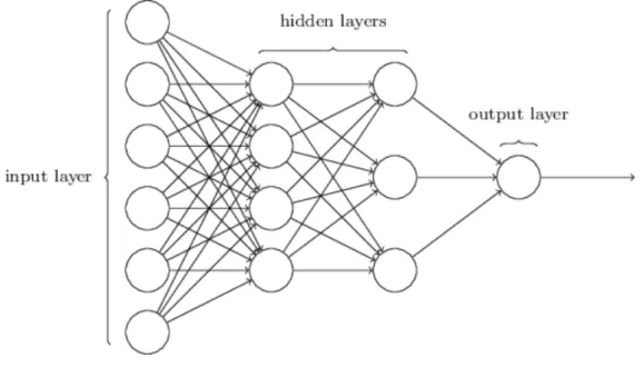
Neural networks are algorithms inspired in biological nervous systems like the brain. They consist in input, hidden and output layers that are connected through sets of neurons, each neuron has a weight, a bias and an activation function associ-ated with it. A neuron when receiving an input performs some calculations using its activation function and outputs the result, which will serve as input to next neuron. deep learning consists in neural networks with multiple hidden layers. Figure 2.1 shows a representation of a neural network with an input layer, two hidden layers and an output layer.

Nowadays, the neural networks architectures used in image classification prob-lems consist in a series of convolutional, pooling and fully-connected layers, used to extract relevant features from the images, followed by one or more fully-connected layers used to perform the classification task. This type of neural networks is called convolutional neural networks (CNN) (Wu, 2017).

Convolutional layers apply convolutions to the input matrix by sliding a filter over it. This filter consists of a kernel, which the width and height are usually the same, a stride and a padding. The stride determines how the filter convolves over the input, for example, if the stride is set as 1, the filter will shift around the input one unit at a time. The padding adds zeros to the input in cases where the filter exceeds the input size, this only happens when the stride is greater than 1. In Figure 2.2 is possible to see a filter with a kernel of size 3x3 and a stride

(25)

Figure 2.1: Neural network representation. Source: (Nielsen, 2015)

of 2 convolving over an input matrix of size 4x4, in this case a padding of 1 is necessary.

Figure 2.2: Convolutional layer filter example.

Pooling layers are used to reduce the size of the image representation and therefore reduce the number of parameters and the computational time in the network. Like the convolutional layers, a pooling layer also uses a kernel and stride, normally with the stride being set to match the width or height of the kernel. The most common type of pooling is the max pooling, this way it keeps the maximum value of the values being process by the kernel.

(26)

Finally, the fully connected layers are normal neural networks layers where all the neurons of the layer are connected to the previous layer. They are commonly the last layers used in a CNN and perform the classification task, where the final layer, the output layer, has one neuron per class.

One of the first CNNs was introduced in (LeCun, Bottou, Bengio, & Haffner, 1998) and it was called LeNet5. The architecture of the LeNet5 consists of seven layers, not counting the input. Three of those layers are convolutional layers use to extract features and the first two convolutional layers are each followed by a subsampling layer (pooling). The third convolutional layer extracted features that are then processed by two fully-connected layers where the classification is performed. The LeNet5 was a pioneer in the deep learning field and the works that followed were based in this work.

In (Krizhevsky et al., 2012) AlexNet was introduced with an architecture that use the principles of the LeNet5 to create a larger neural network. AlexNet is composed by five convolutional layers, which some are followed by max-pooling layers and three fully-connected. The three convolutional layers used filters of size 11x11, 5x5 and 3x3 respectively. The authors of this work performed some introductions like the use of Rectified Linear Units (ReLUs) for the activation functions, which improved the training time, the use of dropout layers and data augmentation to reduce overfitting.

The authors in (Simonyan & Zisserman, 2014) continue the exploration of using CNN for image classification by proposing two new architectures, the VGG16 and the VGG19. Both architectures consist of five convolutional blocks, each block composed by a set of convolutional layers followed by a max-pooling layer, rather than having a pooling layer after each convolution. Instead of using 11x11 filter like the AlexNet, the VGG networks use 3x3 filters. By doing these alterations the authors showed that doing smaller consecutive convolutions have equivalent results to a single convolution with a bigger filter, but with the benefits of using a smaller filter.

Seeking to improve the computational cost of CNNs, the authors in (Szegedy et al., 2015) presented GoogLeNet or Inception. The Inception model contains 22 blocks of layers, that when summed up result in more than one hundred layers, and rather than having the layers stack sequentially, parallel convolutional layers

(27)

compose these blocks. The authors called these blocks with parallel layers Incep-tion module. Each IncepIncep-tion module consist of 1x1, 3x3 and 5x5 convoluIncep-tions, this way the model can decide which is the best convolution operation for each layer. The authors also proposed the use of 1x1 convolutional layer, before each 3x3 and 5x5 convolutions, in order to reduce the number of features and therefore reducing computations.

Continuing from the previous work, some alterations to the Inception network were proposed in (Ioffe & Szegedy, 2015). Batch-normalization was introduced, by normalizing the output of some layers for each mini-batch the model was able to use higher learning rates and consequently reduce training time.

Two new CNN architectures driven from the first Inception network, Incep-tionV2 and InceptionV3, were introduced in (Szegedy, Vanhoucke, Ioffe, Shlens, & Wojna, 2016). The authors propose factorizing large convolutions into smaller ones, showing that a 5x5 convolution is 2.78 times more expensive than a 3x3 convolution, therefore, replacing a 5x5 convolution by two 3x3 convolutions in-creases the performance. Additionally, the authors found that nxn convolutions are equivalent to combination of 1xn and nx1 convolutions, and by doing this factorization the computational cost is reduced. A label smoothing technique is also presented, this technique helps prevent overfitting by preventing the model from becoming too confident about a class.

Around the same time InceptionV2 and InceptionV3 were introduced a new CNN called ResNet was introduced in (He, Zhang, Ren, & Sun, 2016). ResNet consists of a neural network substantially deeper than the previous ones and intro-duced residual learning. Residual learning consists of blocks of layers and shortcut connection where the input of these layers is added to the output. This allows information to be more easily propagated through the network and contributes to a reduction of overfitting. A representation of a residual learning block is showed in Figure 2.3

Inspired by the Inception and ResNet architectures, a hybrid version CNN combining the first two was proposed in (Szegedy, Ioffe, Vanhoucke, & Alemi, 2017) called InceptionResNet. This combination is achieved by adding a shortcut connection, like in the ResNet, to each Inception module. By doing this, although the accuracy did not have significant improvements, the training time was reduced.

(28)

Figure 2.3: Residual learning. Source: (He et al., 2016)

In the same work the authors also present a new version of the Inception network, InceptionV4, which is a simplified version of InceptionV3.

Mobile phones are now more than ever part of our lives, therefore efforts to make these deep learning models able to be used on mobile phones, which have smaller process capabilities and less memory than a normal computer, have been performed. In (Howard et al., 2017), a smaller CNN optimized for mobile applica-tion, called MobileNet, is proposed. MobileNet consists of depthwise convolutions and a 1x1 convolution the authors call pointwise. This pointwise convolution is ap-plied to combine the outputs of the depthwise convolution. Two hyper-parameters that help reduce the model, are proposed as well. The first hyper-parameter, the width multiplier, reduces the number of channels of each layer. The second hyper-parameter, the resolution multiplier, reduces the input image of the model. Most of these CNN architectures were evaluated in the ImageNet Large Scale Visual Recognition Challange (ILSVRC), where as of 2017, the InceptionResNet architecture achieved the best results.

2.1.1.1 Transfer Learning

Most of the CNNs reviewed take a long time to train even on last generation GPUs. However, there is a way to use the knowledge of a CNN gained when trained in a large dataset, like the ImageNet, and adapt it to a similar classification problem. This is called transfer learning.

Transfer learning consists of using a CNN with the parameters, weights and biases obtained when trained in a large dataset, use the first layers for feature extraction and replace the last layers (fully-connected layers) use for classification

(29)

with new layers adapted to the desire classification task. This way there is only need to train the new layers, which will save time and resources (Pratt, Mostow, Kamm, & Kamm, 1991; Pratt, 1993).

In (Yosinski, Clune, Bengio, & Lipson, 2014) the author aims to answer the question "how transferable are features in deep neural networks?". Two problems that affect transfer learning, depending on the layers where features are transferred from, are presented in this work.

The first problem addressed by the authors is "optimization difficulties related to splitting networks between co-adapted neurons", this problem is more accentu-ated when splitting the network in the middle layers then on the bottom or top layers. The second problem is "the specialization of higher layer neurons to their original task at the expense of performance on the target task", this means that the higher layers (i.e. final layers) are more adapted to the original task than the bottom layers, which generalize more easily to new datasets, therefore there are cases where retraining these last layers can be efficient. The authors also confirm that transfer learning is more effective when the base network is trained on a more similar task.

In (Oquab, Bottou, Laptev, & Sivic, 2014) an AlexNet from (Krizhevsky et al., 2012), trained on the ImageNet dataset, is used as the base model for the transfer learning task. The authors propose replacing the last fully-connected layer by two new fully-connected layers that receive as input the output of the penultimate layer of the AlexNet. The first layer of the new layers has size of 2048 and the second layer has a size equal to the number of classes of the new target classification, which in this case are 20 classes. The results show that a transfer learning procedure is effective when using knowledge obtained from a large dataset in a smaller dataset.

A technique to accelerate the transfer of knowledge of one neural network to another was proposed in (Chen, Goodfellow, & Shlens, 2015). This technique it is based on "function-preserving transformations of neural networks" and allows a newer model to contain all the knowledge of an older model and be trained to improve its performance.

(30)

2.1.1.2 Libraries

There are many deep learning libraries that provide an easier implementation, training and use of CNNs. In this section, we review some of these libraries.

A review of several deep learning toolkits and libraries was performed by (Erickson, Korfiatis, Akkus, Kline, & Philbrick, 2017). The first reviewed library is Caffe, developed by Berkeley Vision and Learning Center. It is modular and fast and supports multiple GPUs. There is also a website where Caffe models can be download as well as network weights. One of the disadvantages that the authors of this review point out is that tuning the hyperparameters is a tedious process.

Another library reviewed is TensorFlow, developed by Google. Like Caffe, Ten-sorFlow also supports multiple GPUs. It provides tools for tuning and monitoring performance like TensorBoard.

Theano is another deep learning library, written in python, which has improved performance because of the efficient code base of numpy. It is good to build networks but challenging to create complete solutions.

Keras is a deep learning library written in python that can use either Theano or TensorFlow as backend. It is easier to build and read complete solutions. It is well documented and pre-trained models of common architectures are provided. According to the Keras website (Why use Keras?, 2018), Keras is the second most used deep learning libraries behind TensorFlow. A speed and accuracy comparison between Theano with Keras, Torch, Caffe, TensorFlow and Deeplearning4J was performed by (Kovalev, Kalinovsky, & Kovalev, 2016). The data used in this comparison was from the MNIST database, which is a large dataset of handwritten digits used for training various image classification approaches. The results show that, when increasing the number of neurons, Caffe and Deeplearning4J drop in the accuracy, TensorFlow and Torch increase the accuracy, and Theano with Keras is stable with different number of neurons. In terms of speed, the libraries can be ranked as follows: Theano with Keras, TensorFlow, Caffe, Torch, Deeplearning4J.

2.1.2 Data Augmentation

It is a common mistake to think that a good model equals good results and if you are aiming to improve the results you should consider improving the model.

(31)

Sometimes this can be true, but most times improving the data is better than improving the model. In this section, we provide a view to some of the techniques used to improve the data.

Two of the major problems with low quality data are: not enough data and unbalanced data. Both problems can cause overfitting of the model, but both can be fixed via data augmentation.

A description of the best practices when using CNNs is provided in (Simard, Steinkraus, & Platt, 2003) and the authors conclude that the most important practice is to have a dataset as large as possible. By doing augmentations based on distortions of an original image, the model can achieve better results.

The most common type of data augmentations in image classification problems, and proven to be successful, are techniques such as cropping, rotating and flipping the images. In (Perez & Wang, 2017) show this to be true and propose a method that allows the model to learn which are the best augmentations to perform and achieve better results. This method consists of two networks, one for augmentation and another for classification. The augmentation network creates an augmentation image from two input images of the same class and a loss is calculated to check how similar the image should be to the original images. The classification network is a simple CNN. The authors were not aiming for the best classifier, the goal was to see how data augmentation affects the results of the model.

2.2 Incremental Learning

Many processes and applications need to gain knowledge over new information over time, more specifically, some classification problems require learning new classes progressively. The problem is that most of the classification algorithms cannot perform this task. In this section we take a look at the work performed in incremental learning.

Incremental learning it is not a recent research topic, some of the work per-formed in this area can date back to the end of the eighties. In (Utgoff, 1989), an algorithm is proposed for training decision trees incrementally. The proposed al-gorithm is capable to build a decision tree identical to the one present in (Quinlan, 1986), which is non-incremental, but built in an incremental fashion.

(32)

Neural networks have proven to be an efficient machine learning classifica-tion algorithm. Taking this into account many researchers have tried to imple-ment increimple-mental learning on this type of algorithms. In (Carpenter, Grossberg, Markuzon, Reynolds, & Rosen, 1992), a neural network for incremental learning of analog multidimensional maps is introduced, later in (Polikar, Upda, Upda, & Honavar, 2001), a neural network called Learn++ is introduced. This neural net-work is capable of learning from new data, including examples of previously unseen classes. Like the neural network proposed in (Carpenter et al., 1992), Learn++ does not need to access data used in previous training session, it can learn using only new data. It does this and, simultaneously, does not forget previously gained knowledge.

In (Fuangkhon & Tanprasert, 2009) an "alternative algorithm for integrat-ing the existintegrat-ing knowledge of a supervised learnintegrat-ing neural network with the new training data" is presented. The algorithm uses a counter preserving algorithm to increase the classification accuracy, while maintaining old knowledge as the neu-ral network is retrained with new data. Unlike the previous reviewed works, this approach uses some data used in previous training sessions to help maintain the older knowledge.

One of the reasons incremental learning is a challenging task for neural net-works is their tendency to suffer significant loss of prior knowledge as the network tries to learn from new data. This is called catastrophic forgetting.

Trying to solve the catastrophic forgetting problem, the authors in (Kirkpatrick et al., 2017) present an approach that uses an algorithm called elastic weight con-solidation (EWC) and show that is possible to overcome the catastrophic forgetting problem. EWC allows learning to slow down on weights based on how important they are to previous tasks.

In (Rebuffi, Kolesnikov, Sperl, & Lampert, 2017) the authors showed a new training strategy, that allows incremental learning, called iCaRL. It does not re-quire much data as new classes are added incrementally to the model. ICaRL is made up by three components, a nearest-mean-of-exemplars classifier, a herding-based step for prioritized exemplar selection and a representation learning step that uses distillation to avoid catastrophic forgetting. This method achieved sat-isfactory results, compared to other techniques, when a significantly large number of classes is added to the original model.

(33)

A new training methodology that allows CNNs to learn new classes from new unseen data is proposed in (Sarwar, Ankit, & Roy, 2017). This methodology uses principals of transfer learning by updating a network for a set of new classes using the initial part of the base network. It consists of a mechanism able to identify how many of the base network layers weights and parameters can be shared when adding new classes. When training the model for new classes, new layers are created which become a branch of the existing network.

Mondrian forests are a type of random forests that can be used both for classifi-cation (Lakshminarayanan, Roy, & Teh, 2014) and regression (Lakshminarayanan, Roy, & Teh, 2016). They consist of an ensemble of decision trees based on Mon-drian processes that can be trained incrementally, called MonMon-drian trees.

Most of the decision trees, that also support incremental learning, usually perform splits on the leaf nodes when being trained incrementally. Mondrian trees also perform splits on leaf nodes when updating their knowledge with new data, however, Mondrian trees also perform two more operations. Therefore, there are three different ways to update Mondrian trees:

• A new split "above" an existing slip. • Extension of an existing split.

• Split of a leaf node into two new nodes.

In a training session with new data the Mondrian tree is updated, and an algorithm decides which operation of three mention above is used for each node. This decision is made considering the split cost of each node.

To perform a prediction of a certain data input, each Mondrian tree contained in the forest determines the probability of the input belonging to every one of the existing classes. After the average of the trees predictions is calculate and the class with the highest probability corresponds to the predicting class.

Although Mondrian forests can learn from new unseen data the authors of (Lakshminarayanan et al., 2014) do not experiment adding new classes to the model. In (Narr, Triebel, & Cremers, 2016) an extension of the Mondrian forest algorithm for classification of images is presented. This approach can learn new unseen classes. Some alterations to the original implementation were performed.

(34)

In the original implementation of the Mondrian forest when all the labels of a certain node are the same, no split is performed for that node. This "pause" operation, as the authors call it in their work, allows the comparison between Mondrian and other random forest implementations. However, in (Narr et al., 2016), the authors chose to remove this operation and instead define a threshold to limit the maximum number of samples with the same label that a leaf node can have.

2.3 Quality Control

Quality control using machine learning techniques has been a hot research topic for a few years. Earlier work performed in this area used Fourier analysis to detect defects in fabric (Chan & Pang, 2000). Using white fabric for the experiences, the system was able to detect four different types of defect by applying Fourier transforms to the images and analyzing the frequency spectrum.

In (Kumar & Pang, 2002) the frequency spectrum is also analyzed to de-tect defects but instead of using Fourier analysis, the authors used Gabor filters. Two approaches are presented, a supervised and an unsupervised defect detection. The difference between the two is that in the supervised approach, information about the orientation and the size of the defects is given. This information makes spectrum-sampling of the spatial-frequency plane unnecessary, allowing the sys-tem to work with just one Gabor filter. As for the unsupervised approach there is a need to use multiple filters so that the system can get information about the orientation and size of the defects.

The same authors then proposed a different approach for this problem using a feed forward neural network. This neural network was used to classify feature vectors of pixels extracted from images (Kumar, 2003). Despite proposing a feed forward neural network for defect detection, due to the computational cost of this type of networks at the time of the work, the authors also propose a linear neural network with a lower computational cost and instead of classifying 2-D images the input was reduce to 1-D vectors.

Another approach of detecting defects is to calculate and evaluate the degree of similarity between an image with defect and an image with no defect. In (Tsai & Lin, 2003) this approach, a normalized cross correlation to calculate the degree

(35)

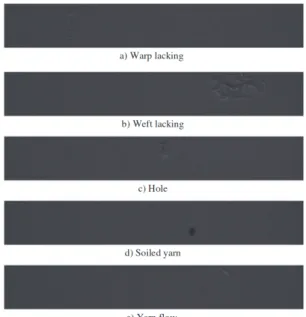
of similarity is utilized. A sliding window is used to process the image, but it size affects the computational efficiency and the effectiveness of the detection. Taking this into account the authors proposed a sum-table scheme that allows the calculation of the normalized cross correlation to be invariant to the window size. More recently in (Çelik, Dülger, & Topalbekiroğlu, 2014) it is proposed a method for defect detection as well as defect classification. For the defect de-tection it was used a wavelet transform, as for the classification task it was used a feed forward neural network. The system was able to detect effectively five types of defect: warp lacking, weft lacking, soiled yarn, hole and yarn flow. Figure 2.4 shows examples of these types of defect.

Figure 2.4: Fabric defect types. Source: (Çelik et al., 2014)

In (Li et al., 2014) a mobile phone cover glass defect detection is presented, and even though it is for glass defects and not fabric defects like the previous reviewed works, the principles are the same. The propose system consists in a defect inspection system based on the Principal Component Analysis (PCA) and is capable of identify five cover glass defects.

Works such as (Weimer, Scholz-Reiter, & Shpitalni, 2016) and (Wang, Chen, Qiao, & Snoussi, 2018) have used CNN to perform quality control and defect detection tasks. In the first work, four different CNN architectures are proposed and trained to identify six types of defects. Each architecture had a different number of convolutional layers with the results showing that, in this case, adding layers increases the detection accuracy. In the second work a CNN able to detect

(36)

six types of defects is also proposed. The architecture of this CNN consists of 11 layers, five of which are convolutional layers and two pooling layers.

Additional work regarding the topic of quality control and defect detection can be found in (Kumar, 2008) and (Ngan, Pang, & Yung, 2011).

(37)

Chapter 3 Quality Control System for Clothing

Manufacturing

In this chapter, we describe the quality control system for clothing manufacturing (QCSCM) proposed in the first chapter as the objective of the present work. The purpose of the QCSCM is to detect defects on clothing items. This is achieved by using a classification model supporting incremental learning. This classifi-cation model can, however, be easily adapted to other contexts.

The present work was developed to be used by a real clothing factory and was made under the collaboration ISCTE-IUL/INOV INESC Inovação. INOV wants to create a commercial system to help manufacturing companies in their quality control processes, in this case oriented to clothes. Based on a defined client, INOV defined a set of requirements that the system should fulfill based on training sets and a machine learning approach. These requirements are as follows:

• A system capable of detecting defects on clothing items using

pic-tures. The system outputs a binary classification, defect or no defect,

based on the classification of the clothing items components.

• A mobile application to take the pictures of the clothing items and be used by the quality control officers to perform their quality

control tasks. The system is fed by the quality control officer using the

(38)

Chapter 3. Quality Control System for Clothing Manufacturing

• Increase the speed of the quality control processes and the

percent-age of detected defects. For the system to be useful, it should improve

the performance of the quality control processes.

• The ability of the system to learn from new data, as new

compo-nents of clothing items are created. The system must learn new classes

maintaining its previous knowledge. The quality control officer creates the new data using the mobile application and feed the system in a collaborative way.

INOV also defined the types of defect this system aims to detect on a clothing item. A clothing item is made up by a set of components, such as buttons, pockets, stamps, etc. Therefore, a defect can be one of two types:

• Wrong component. • Missing component.

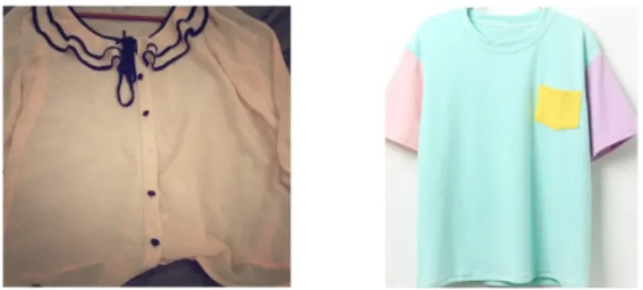
Figure 3.1 shows an example for each type of defect. The one on the left corresponds to a shirt with a missing button (missing component) and the one on the right shows a t-shirt with a yellow pocket instead of a pink pocket (wrong

component).

Figure 3.1: Examples of the two types of defects. Missing component on the left, wrong components on the right.

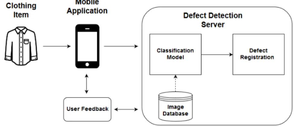
Considering the requirements and the types of defect, the QCSCM architecture was defined in Figure 3.2. Using a client-server model approach, the QCSCM consists of a mobile application and a server, we called Defect Detection Server (DD Server). The mobile application is used to take pictures of the clothing items and the DD Server is responsible for processing and storing the pictures, detect

(39)

the defects making use of the classification model and finally, register the defects. To improve the QCSCM performance a user feedback approach was also defined.

Figure 3.2: QCSCM general architecture

The responsibility of the quality control in the factory lies with a group of factory workers called quality control officers. The function of the quality control officers is to detect defects on the clothing items, register them and decide whether to send the clothing item back to the manufacturing process, remove the clothing item from production, or continue to the next production step. A clothing item is sent back to the manufacturing process if a repairable defect is detected and is removed from production if an unrepairable defect is detected.

To execute their function, the quality control officers use the mobile applica-tion to take pictures of the clothing items and create bounding boxes around the components that compose a clothing item. This information is sent to the DD Server that crops the content of the bounding boxes to create the images

of the components. These images of the components are classified by the

clas-sification model and the results are compared with the product data sheet to see if there is a defect or not. Finally, the classifications of components are sent back to the mobile application being used by the quality control officer.

A product data sheet is information associated to each model produced by the clothing factory. The product data sheets are defined by the clothing factory every time a new clothing item model is created. The information present in the product data sheet information consists of a list of specifications and components that compose a clothing item. Its structure is as follows:

(40)

Chapter 3. Quality Control System for Clothing Manufacturing • Size.

• Color. • Fabric.

• List of components.

The QCSCM focuses on the list of components specification. All the clothing items have an identifier corresponding to a product data sheet, so when a cloth-ing item is gocloth-ing through a quality control process the system can know which components it has to identify.

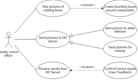
As in any other manufacturing business, in a clothing manufacturing business new products and components can be created. Therefore, the QCSCM uses a classification model which has the ability of learning new classes incrementally. The responsibility of creating images of the components to train the classification model also relies on the quality control officers. To create images of the new classes or even more images of old classes, the quality control officer can choose an option in the mobile application to use the pictures it took to train the classification model instead of using the pictures for the defect detection process. The quality control officer can also create more images by confirming or correcting the classifications it received from the DD Server, this is the user feedback feature. In Figure 3.3 we defined a use case diagram that explains the actions the quality control officer performs using the mobile application.

Figure 3.3: Use case diagram of the quality control officer actions using the mobile application

(41)

3.1 Defect Detection Server

The first main component of the QCSCM is the DD Server responsible for feeding the classification model with images of the clothing items components. The DD Server must perform the following tasks:

1. Pre-process the images of the components it receives from the

mo-bile application used by the quality control officers. This task of

pre-processing the images consists of cropping the bounding boxes of the pictures taken by the quality control officers creating images of the com-ponents. These images of the components are then resized and, in case of training, new images are created using data augmentation techniques. The pre-processing task is necessary so that the classification model can perform its tasks.

2. Predict the classes of these components. In this second task, the classification model present in the DD server predicts the classes of the com-ponents it received from the quality control officers.

3. Compare the results with the product data sheet and save the

results. After the classifications are made the DD server performs the third

task of comparing the results with the product data sheet. If the identified components match with the ones present on the product data sheet it means no defect was detected and nothing needs to be registered. If they do not match, it means a defect has been detected and the DD Server performs the

defect registration.

4. Store pictures of the components and train the classification model

with new data. This fourth and final task is only performed if a quality

control officer selected the option of using the pictures to train the clas-sification model. The DD Server after cropping the bounding boxes of the pictures taken by the quality control officers, saves the content of the bound-ing boxes (images of the components) along with the correspondbound-ing labels in a database. If enough images of the components are stored in the database, the training of the classification model is performed.

(42)

3.1.1 Image Database

When a quality control officer sends pictures of clothing items with bounding boxes around the components it has to select the option of the task to execute. If the selected option is to use the pictures to train the classification model, the images of the components of the clothing items need to be stored. In this section we describe the image database represented in Figure 3.2 as a module of the DD Server.

After the pictures of the clothing items are processed and the images of the components are created, the DD Server saves the images according to their classes. Each class has an associated directory where all images corresponding to that class are stored. The names of the directories serve as labels for the images when the classification model is trained.

This image database allows the creation of the dataset that is used to train the classification model. Every time the classification model needs to be trained, the DD Server loads the images and labels from the image database and feeds them to the classification model.

The image database also contains a list of the classes and the number of new images available from each class. This list is used to check if there are enough images to train the classification model and it is also sent to the quality control officers when they want to label the components of the clothing items using the mobile application.

3.1.2 Defect Registration

The defect registration is represented in Figure 3.2 as a module of the DD Server. It is performed after the classification model classifies the components that are sent to the DD Server and after the results of the classification are compared with the product data sheet to check if there are defects. In case of a positive defect detection, the type of the defect, missing component or wrong component, also needs to be registered. For example, let’s assume we have a clothing item that is supposed to have three black buttons and one silver zipper, but the classification model returns two black buttons and one silver zipper. In this case the DD Server would register the defect as missing component along with the components that are missing, in this case a black button.

(43)

Another example using the same clothing item, the classification model returns three black buttons and a golden zipper. In this case the DD Server would register the defect as wrong component and register the misplaced component, in this case a golden zipper instead of a silver zipper.

Apart from the image database and the defect registration the other main module of the DD Server is the classification model. However, due to its im-portance we decided to describe the classification model in a separated section.

3.2 Mobile Application

The second main component of the QCSCM is the mobile application, developed using Android Studio. It is supported by the Android versions 4.1. and above. The quality control officers use this mobile application to take pictures and create bounding boxes around the components that make up the clothing items. The mobile application consists of a simple user interface, that displays the pictures taken by the quality control officer using the mobile phone camera. It allows the quality control officers to choose whether to use the pictures to detect defects or to use them to train the classification model. The reason of using a mobile application to take pictures instead of a fixed camera is because this way allows the quality control officers to walk around the factory and take pictures of the clothing items in different production steps.

To create the bounding boxes all the quality control officer must do, is drag a finger over the picture and surround the component. By doing this the application stores four coordinates of the image per bounding box. This set of four coordi-nates consists of two x coordicoordi-nates (width) and two y coordicoordi-nates (height). When creating the bounding box, the quality control officer can choose, through a check box, if he wants to classify the component or if he wants to create new data for training. This check box will determinate which process will be executed by the DD Server, the defect detection process or the training process.

For the mobile application to send the pictures to the DD Server, the pictures need to be converted to bytes as well as information about the bounding boxes. After receiving the bytes from the mobile application, the DD Server converts them back to the original format.

(44)

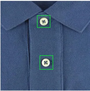
Regardless of whether the quality control officer chooses to use the pictures it took to train the classification model or to perform defect detection, they must always create bounding boxes around the relevant components present in the pic-tures. Figure 3.4 shows an example of a picture of a shirt and the bounding boxes around the components that will be classified.

Figure 3.4: Bounding boxes example

During the creation of new data to train the classification model, after drawing bounding boxes around the relevant components in the picture, the quality control officers must label each component with the corresponding classes. The classes can be chosen from a list of existing classes or, if the object consists of class not present in the classification model, the quality control officers can create a new class that will be added to the list of existing classes.

During the defect detection process, after receiving the pictures taken by the quality control officers, the DD server sends back the results of the classification model – classified components – so that the quality control officers can give feed-back on the classifications made. This interaction between the DD Server and the mobile application – user feedback – allows the quality control officer to cor-rect wrong classifications made by the classification model of the DD Server and confirm the correct ones.

The user feedback feature is easy to execute, after performing a defect de-tection process using the mobile application and receiving the results from the DD Server, the quality control officers can perform the necessary corrections by

(45)

clicking on the bounding boxes with the wrong predictions and select the correct label from a list of the existing classes.

After the corrections are made, the quality control officer sends the information again to the DD Server and new images are created to train the classification model. Although in an initial stage of the QCSCM life-cycle it is useful that the quality control officer performs this feature, it is not mandatory.

Using the feedback from the quality control officers, the DD Server corrects the registered defect and creates new training data that will be used in future training sessions. So, basically the user Feedback feature is mainly another way to trigger the training process of the DD Server. Its implementation consists of allowing the quality control officers to change the wrong labels of the bounding boxes by clicking on them via the mobile application or confirming the results using an application button that will send a Boolean value set to true back to the server and initializes a new training process.

This user feature contributes to better training and subsequently better perfor-mance of the classification model present in the DD Server. This is only possible thanks to the ability of the classification model to learn incrementally.

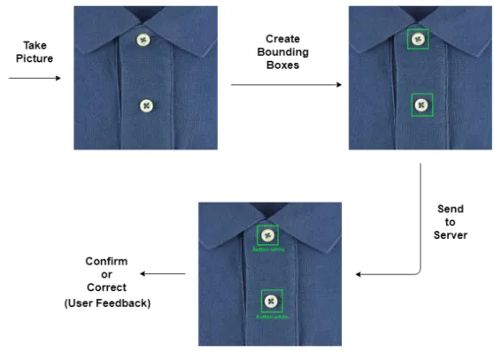
Figure 3.5 shows all the steps a quality control officer goes through during the defect detection process using the mobile application, with a last step being the execution of the user feedback.

3.3 Classification Model

In this section, we propose a classification model for images that can learn incre-mentally as new classes are created and be used in a quality control system to perform defect detection.

The proposed classification model is divided in a feature extraction model and classifier with incremental learning abilities, as seen in Figure 3.6. Although in this work we used the classification model to classify components of clothing items, it can be adapted to other quality control environments.

The feature extraction model consists of a pre-trained CNN that extracts important features from the content of the images. After the extraction, the

(46)

Figure 3.5: Quality control officer process of defect detection using mobile application

Figure 3.6: Classification model architecture

images are classified by the classifier using the extracted features and modi-fied version of the Mondrian forest algorithm that supports incremental learning (Lakshminarayanan et al., 2014). We chose this architecture for the classification model, because by using the principles of transfer learning, we can combine the benefits of using a CNN to extract relevant information from an image with the ability of Mondrian forest to learn incrementally.

(47)

3.3.1 Feature extraction model

The idea of using a feature extraction model in the classification model was to make sure that the classifier only needs to process and classify relevant information and to reshape the input of the classification model from a three-dimensional array (an image) to a one-dimensional array that can be fed to the classifier. We chose to use a CNN as the feature extraction model because of the recent state-of-the-art results of this type of neural networks when it comes to image classification problems. Figure 3.7 shows a simple CNN architecture and how it extracts relevant features from an input image and converts them into a feature array.

Figure 3.7: CNN architecture and feature extraction. Adapted from: (Britz, 2015)

As we seen in chapter 2, there are many CNN architectures and these architec-tures can be trained in very large datasets to create knowledge and know which are the relevant features that can be extracted from an image. This knowledge consists of using the best weights and biases for each layer of a CNN and it can be adapted to similar image classification problems using transfer learning.

3.3.2 Classifier

The function of the classifier is to classify the images of the clotting items using the features extracted from the feature extraction model. As any other classification algorithm, the classifier present in the classification model needs to be trained with data relative to the classes it wants to classify. However, our classifier must be able to learn incrementally new classes and gain knowledge from unseen data.

Incremental learning is the ability of an algorithm to gain knowledge from

(48)

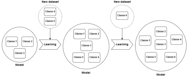
increase of classes by training the model with data of new unseen classes, or an increase of knowledge of the old classes by training the model with new data from old classes. Figure 3.8 shows a representation of how a model can learn incrementally.

Figure 3.8: Incremental learning.

As said before, the classifier present in the classification model consists of a Mondrian forest presented in (Lakshminarayanan et al., 2014). A Mondrian forest is a type of random forest that can learn incrementally. The input of the Mondrian forest is a one-dimensional array, therefore, it is able to train with the feature arrays extracted using the feature extraction model. In the next chapter we detail how we developed the classification model and how our classifier (Mondrian forest) behaves when classifying the feature arrays extracted using different CNN architectures.

(49)

Chapter 4 Development of QCSCM

In this chapter, we present the tools and techniques used to develop the classifica-tion model and the QCSCM as well as detailed informaclassifica-tion on the steps we took during the development.

4.1 Classification Model

As seen in Figure 3.2, the classification model, described in section 3.3, is a com-ponent of the DD Server of the QCSCM. However, due to its importance and the work we had to develop it, we describe its development in a separated section first. This classification model was developed to classify objects that correspond to the components of the clothing items and would then be implemented in the DD Server of the QCSCM.

As shown in Figure 3.6 in the previous chapter, the classification model is made up by a feature extraction model and a classifier. The feature extraction model consists of a pre-trained CNN without the last layers (fully-connected layers), which are normally use for the classification task. As for the classifier it consists of a modified version of the Mondrian forest algorithm. By doing this, we follow the principle of transfer learning, but instead of adding new layers and trained them with new data, we use the Mondrian forest algorithm which is capable of learning incrementally.

(50)

Chapter 4. Development of QCSCM

4.1.1 Feature Extraction Model

As defined in the previous chapter, to extract relevant features from the input images we use a pre-trained CNN. The Keras Library provides many CNN archi-tectures already pre-trained on the ImageNet dataset that can be adapted to this problem.

The ImageNet Dataset (Deng et al., 2009) is a very large image database containing more than one million images of objects divided in 1000 classes. The knowledge gained by a CNN when trained with this dataset can be easily adapted to similar image classification problems.

In order to set some baseline results and due to the lack of real images of components of clothing items, we used the Cifar-10 dataset (Krizhevsky & Hin-ton, 2009) to perform some experiments and check if the classification model can perform well in an image classification problem. The Cifar-10 dataset consists of 60000 images in 10 classes, with 6000 per class. Of these images, 50000 are used for training and 10000 are used for test. Each image consists in a 32x32 color image. The 10 classes are the following: airplane, automobile, bird, cat, deer, dog, frog, horse, ship, truck.

To use one of the CNN architectures in Keras as a feature extractor, all we have to do is load the desired CNN architecture with the weights obtained during the ImageNet training, remove the last fully connected layers used for classification and process the input images through the network to extract the features. Finally, we save these features in arrays that will serve as the input of the classifier.

4.1.1.1 Why extract features?

Why should we use a CNN to extract features of the images of the components of the clothing items and then classify these features instead of classifying directly the images? In this section, we answer this question and show the importance of feature extraction.

If we did not used a CNN as features extractor, the classifier would use the raw images as input instead of a feature array. For us as humans it is easy to look at an image and understand what it represents, the same cannot be said when we look at a feature array extracted from a CNN.

(51)

Figure 4.1 shows a raw image of a clothing item component on the right and its corresponding feature array on the left extracted using InceptionResnet. We converted the 1536 size array to an 32x48 matrix for easier interpretation.

Figure 4.1: Representation of feature extracted using InceptionResnet

If we look at the representation of the extracted features in Figure 4.1 it is hard to understand what it represents and difficult to extract some useful infor-mation, just by looking at it. To compare how the classifier, Mondrian forest, performed on classifying the raw images versus classifying the features extracted from the feature’s extractor, we performed an experiment using python to calcu-late the classification test accuracy of the two methods. The accuracy is a metric for evaluating classification models and measures the fraction of the number of correct predictions (Nc) over the total number of predictions (Np) (Classification:

Accuracy, 2018):

accuracy = N c

N p. (4.1)

Table 4.1 shows the results of this experiment on the Cifar-10 dataset and, as we can see, the classification of CNN features is much better than the classification images. This can be explained for two reasons, the first one being the fact that our classifier receives as input a one-dimensional array, therefore, to feed the images to the classifier they had to be converted from a three-dimensional array to a one-dimensional array. This is not efficient because this way the image loses the relationships between pixels. On the other hand, a feature array extracted from a CNN is already a one-dimensional array.

Raw images classification vs CNN features classification Number of classes Raw images InceptionResnet features

10 0.38 0.85

(52)

The second reason for the classifier performing better when classifying features is because the layers of the CNN are trained to extract relevant information from the images and pass this information through the network. This results in a feature array containing mainly useful information, allowing a better classification.

4.1.1.2 CNN Architectures

To choose which CNN to use in the final version of the classification model, we performed some experiments on some of the architectures provided by the Keras library. The chosen architectures were: VGG16, MobileNet-V1, Inception-V3, ResNet50 and InceptionResnet-V2.

The VGG16 and the MobileNet architectures were chosen because the feature arrays they output are of size 512 and 1024, respectively. Therefore, the com-putational cost and time of training our classifier with these features is smaller when compared to the feature arrays of size 2048 of the ResNet and the Inception architectures, and the feature array of size 1536 of the InceptionResNet. These last three architectures were chosen because of their state-of-the-art results.

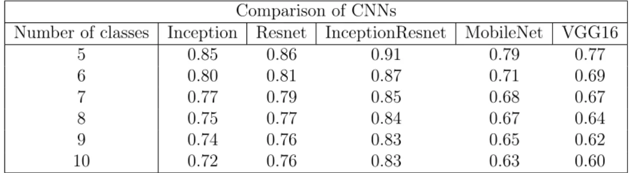
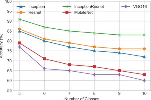
We created a python script to train the classifier on features extracted from the Cifar-10 dataset using each of the selected CNN architectures in an incremental fashion, first we trained it with 5 classes and the we added classes progressively until the classifier was trained for all 10 classes of the dataset. The number of Mondrian trees of Mondrian forest was set to 100. We used this number of trees because it is a common value used in decision forests (Lakshminarayanan et al., 2014). Table 4.2 shows a comparison of the classification accuracies for each set of features using our classifier.

Comparison of CNNs

Number of classes Inception Resnet InceptionResnet MobileNet VGG16

5 0.85 0.86 0.91 0.79 0.77 6 0.80 0.81 0.87 0.71 0.69 7 0.77 0.79 0.85 0.68 0.67 8 0.75 0.77 0.84 0.67 0.64 9 0.74 0.76 0.83 0.65 0.62 10 0.72 0.76 0.83 0.63 0.60

Table 4.2: Comparison of CNNs features classified with Mondrian forest As the Table 4.2 and Figure 4.2 show, for all CNN architectures, the accuracy decreases when new classes are added. The InceptionResnet shows the best results,