Relatório de Estágio na Inficon AG e na PT Inovação & Sistemas

(1)

Mestrado em Engenharia Eletrotécnica, Ramo de

Eletrónica e Telecomunicações

Relatório de Estágio na Inficon AG e na

PT Inovação & Sistemas

Andreia Gama

(2)

(3)

Mestrado em Engenharia Eletrotécnica, Ramo de

Eletrónica e Telecomunicações

Relatório de Estágio na Inficon AG e na PT

Inovação & Sistemas

Relatório de Mestrado realizado sob a orientaçãodo da Doutora Mónica Jorge Carvalho Figueiredo, Professora da Escola Superior de Tecnologia e

Gestão do Instituto Politécnico de Leiria

Andreia Gama

(4)

(5)

Acknowledgements

This project would not have been possible without the kind support and help of many individuals. I would like to extend my sincere thanks to all of them.

First and foremost, I would like to thank Inficon AG and PT Inovação & Sistemas for providing me the opportunity to integrate their teams, learn from profissionals and work with state of the art tecnhonology.

Regarding to the Inficon AG, I would ike to express my gratitude the members of the Reaserch & Tcnhology team for promptly helping whenever was needed. Special thanks to my mentor, Martin Wüest for is guidance and support.

Regarding to PT Inovação & Sistemas, I would like to express my gratitude to the members of the Microelectronics development group, their help and support have been instrumental in the successful completion of this project. I would also like to give a special thanks to my mentor, João Puga Faria for his crucial guidance.

I’m specially grateful to my family and friends, particularly my mother, for their love, un-shakable patience and encouragement, which were fundamental to face all the difficulties.

(6)

(7)

Abstract

This document focuses the projects developed during two independent internships, which were carried out at Inficon AG and PT Inovação & Sistemas. Since the research areas of both internships are unrelated, individual abstracts are presented.

Inficon AG

The introduction of new products in the market demanded for a tool that could be used both for testing and marketing demonstrations This project outlines the design and development of a graphical user interface to retrieve and process data from standard vacuum gauges, using both the RS232 and the EtherCAT communication protocols, and from the new fast gauge just using the EtherCAT protocol. The GUI is written in a graphical programming language and runs in LabVIEW.

Particular attention is paid to the real-time accuracy, specially of the data provenient from the new gauges, due to their very fast sampling rate. The implementation of com-munication with the EtherCAT supporting gauges is also object of great focus.

Additionally, the precision of the capacitance diaphragm gauges manufactured by Infi-con is compromised by zero drift. Several researches were previously performed in order to understand the drift, model and eliminate it. However none of them presented a con-clusive and reliable solution. This study extends these researches focusing on long-term zero drift compensation using Kalman filters, as they proved to be very efficient for a wide range of applications.

(8)

The exponential growth of Internet users and introduction of multimedia services, which demand high throughputs, is challenging the current IP routers. The bottleneck is the lookup technique used to obtain the longest prefix match. There are several hardware-based solutions, which can be classified into three categories: trees, tries and hashing. The present project approaches IP lookup problem and provides an hybrid architecture, which conjoins exact matching with an uni-bit trie. Such solution aimed a throughput of 10 Gbps and seamlessly implementation in a FPGA. The system was tested under simulated and real time environments, and for the worst case scenario a lookup rate of 14.8 million pps was measured.

(9)

List of Figures

Figura I.2.1 EtherCAT medium access mechanism [6] . . . 9

Figura I.2.2 EtherCAT frames [2] . . . 9

Figura I.2.3 EtherCAT logical addressing [2] . . . 10

Figura I.2.4 EtherCAT master architecture [3] . . . 11

Figura I.2.5 EtherCAT slave arcitecture[3] . . . 12

Figura I.3.1 Block diagram of the measurement system . . . 13

Figura I.3.2 Data path between LabVIEW and TwinCAT . . . 15

Figura I.3.3 Flowchart of the PLC program . . . 16

Figura I.3.4 Example of the FIFOs access control . . . 18

Figura I.3.5 Flowchart of the functions which read/write EtherCAT parameters 20 Figura I.3.6 Flowchart of the function EcatReadArray . . . 21

Figura I.3.7 Flowchart of the function EcatAckReadLow . . . 22

Figura I.3.8 Flowchart of the function EcatStartPLC . . . 22

Figura I.3.9 Flowchart of the sequence implementing the functions related to the data provided by the RS232 gauge . . . 24

Figura I.3.10 Flowchart of the sequence implementing the functions related to the data provided by the EtherCAT gauges . . . 26

Figura I.5.1 Measurement principle of the capacitance-diaphragm gauges . . 30

Figura I.5.2 Shear of the glass solder simulated by the Burguer model [3] . . 30

Figura I.5.3 Algorith of the Kalman filter [21] . . . 32

Figura I.5.4 Long-term drift . . . 33

Figura I.5.5 Output signals of the 1st order discrete Kalman filter . . . 35

Figura I.5.6 Drift compensated signals and respective standard mean error . 35 Figura I.5.7 Output signals of the 2nd order discrete Kalman filter . . . 36

Figura I.5.8 Drift compensated signals and respective standard mean error . 36 Figura II.2.1 Ethernet Frame . . . 46

(14)

Figura II.3.1 Router’s Architecture . . . 57

Figura II.3.2 Flux Diagram of the Lookup Algorithm . . . 58

Figura II.3.3 Uni-bit Trie Configuration Example . . . 60

Figura II.3.4 Block Diagram of the Implemented Hardware . . . 60

Figura II.3.5 Flux Diagram of the System’s General Tasks . . . 61

Figura II.3.6 RAM Access Shared by Multiple Machines . . . 63

Figura II.3.7 Block Diagram of the Uni-bit Trie Engine . . . 64

Figura II.3.8 Test Scheme . . . 66

Figura C.1 Arria V ALM [16] . . . 107

Figura C.2 HDL Designer Graphic Interface . . . 108

Figura C.3 ModelSim Graphic Interface . . . 108

(15)

List of Tables

TabelaI.1.1 Functional requirements and respective priorities . . . 6

TabelaI.1.2 Non-functional requirements . . . 6

TabelaI.3.1 Description of the PLC inputs/outputs . . . 17

TabelaI.3.2 Main variables of the PLC program . . . 19

TabelaI.3.3 Resume of all the functions of the DLL EcatLavViewCom . . . . 20

TabelaI.5.1 Configuration of the developed Kalman filters . . . 34

TabelaII.1.1 Activity Schedule . . . 44

TabelaII.2.1 Example of a Routing Table . . . 51

TabelaII.3.1 (a)Table of Direct Forwarding; (b) Table of Uni-bit Trie . . . 59

(16)

(17)

List of Acronyms

ADS Automation Device Specification CGD Capacitance diaphragm gauges CIDR Classless Inter-Domain Routing CRC cyclic redundancy check

CSMA/CD Carrier Sense Multiple Access With Collision Detection DC Distributed Clock

DDR3 Double Data Rate type 3 memory DLL Dynamic-link library

DSCP Differentiated Services Code Point ECN Explicit Congestion Notification ENI EtherCat network information EOF End-of-frame

ESC EtherCAT Slave Controller ESI EtherCat Slave Information ESI EtherCAT Slave Information ESM EtherCAT State Machine

EtherCat Ethernet for control Automation Technology FMMU Fieldbus Memory Management

FPGA Field-programmable gate arrays FSC Frame check sequence

IFG interframe gap

IHL Internet Header Length IP Internet Protocol LAN Local area network LLC Logic link control LUT lookup table

(18)

P2P Peer-to-Peer PDO process data object

PLC Programmable logic controller QoS Quality of Service

RIP Routing Information Protocol SDO Service data object

SFD Start frame delimiter SII Slave Information Interface SOF Start-of-frame

TCAM Ternary Content-Addressable Memory TTL Time to Live

VLAN Virtual LAN VOD Video on demand VOIP Voice-over-IP

(19)

Introduction

The present document describes the projects developed during two curricular intern-ships, which were carried out at Inficon AG and PT Inovação & SIstemas. The research fields of both internships were unrelated, therefore they will be presented independently. Inficon AG is a multinational company which provides instruments for analysis, mea-surement and control in industrial vacuum processes. The internship was incorporated into the IAESTE programme, under the orientation of Dr. Martin Wüest, and enrolled between 29 July 2013 and 20 December 2013. The original main task was the study and development of an online drift compensation system for capacitive pressure sensors. However, it became a complementary project with low priority, as the introduction of two new products in the market, the EtherCAT interface in several pressure sensors and the high speed capacitor pressure sensor, demanded the development of a tool that could be used by the research team for testing and by the sales team for marketing demonstrations. Since a non-disclosure agreement was not signed all the developed code is presented in the annexes.

PT Inovação & Sistemas is a telecommunications company focused on the development of networking systems. The internship was enrolled between 3 February 2014 and 2 Au-gust 2014, under the orientation of João Puga Faria and supervision of Joaquim Serra. The project was incorporated into the microelectronics group and comprised the de-velopment of an FPGA-based IP router. This document only provides an architecture overview and the obtained results, since a non-disclosure agreement was signed and sen-sitive information can not be shared.

Document Organization

This document is dived into two distinct parts: part I presents all the work developed during the intersnhip at Inficon AG; and part II describes the project developed at PT

(20)

In-• Part I is composed by five chapters. The first four chapters describe the main project developed, the graphic tool for testing the new products, while the last chapter is dedicated to the drift compensation study.

– Chapter 1 - Introduction - This chapter describes the functional and

non-functional requirements of the tool.

– Chapter 2 - Fundamental Concepts - In this chapter the EtherCAT

proto-col is the subject of study, since it is fundamental for a proper understanding of the developed work.

– Chapter 3 - Methodology - This chapter describes the target measurement

system and all the developed code algorithms.

– Chapter 4 - Conclusions - In this chapter the conclusions obtained from this

project are presented.

– Chapter 5 - Zero Drift Compensation - This chapter is dedicated to the

drift compensation project. It comprises all the fundamental concepts needed to properly understand the developed work; the implementation methodology; analysis of the results; and the obtained conclusions.

– Annexes A and B, presented in part III, comprise all the developed code.

• Part II is organized as follows:

– Chapter 1 - Introduction - This chapter describes the main goals of the

project and presents the activity schedule.

– Chapter 2 - Fundamental Concepts - In this chapter are explained some of

the concepts that are fundamental for a proper understanding of the developed work. The three main subjects are Ethernet, IPv4 and lookup techniques.

– Chapter 3 - Methodology and Results - This chapter describes the lookup

algorithm implemented. The test used to validate the developed hardware is also explained.

– Chapter 4 - Conclusions - In this chapter the conclusions obtained from this

project are presented.

– Annex C, presented in part III, comprises a short overview about FPGAs,

(21)

Part I.

Inficon AG

(22)

(23)

I.1. Introduction

Nowadays the RS232 is the main communication protocol used by vacuum gauges. How-ever, it presents several issues, the most relevant ones being the high power consumption resultant of the large voltage swings; the limitations imposed on the noise immunity and transmission distance by the common signal; and the low speed. To overcome these limitations the new vacuum gauges are equipped with EtherCAT interface, an Ethernet based industrial network protocol. This one is characterized by very high speed (100 Mbps); low jitters and latency, being capable of handling real-time applications; flexi-ble topology; and high cost-effectiveness. Another major advantage of EtherCAT is the object dictionary structure, as it allows to easily read/write several gauge parameters. All the objects in the dictionary can be written/read with SDO (Service Data Objects) services (i.e. CANopen asynchronous mailbox communications) and many of them can be mapped in PDOs (Process Data Object) for a fastest cyclic communication. Both PDOs and SDOs are accessed via index and sub-index.

To increase the real-time precision of the pressure measurements, a new vacuum gauge was developed, which samples new data in periods of 700 microseconds (1.428kHz), be-ing 43 times faster than standard 30 milliseconds gauges.

The main objective of this project is to develop a graphical user interface based on the one from the X-Chip Monitor project [15], that would allow to retrieve and process data provenient from standard vacuum gages, using both the RS232 and the EtherCAT com-munication protocols, and from the new fast gauge just using the EtherCAT protocol. With this tool It’s intended to verify both the increased precision of the new fast gauge and the advantages of the use of EtherCAT over RS232 as communication protocol.

(24)

I.1.1. Requirements

In order to optimize the development process of the proposed software, an analysis of the requirements in terms of its functionality and priority (high, medium and low) was performed. The functional requirements and respective priorities are shown in table I.1.1, while table I.1.2 presents the non-functional requirements.

Table I.1.1.: Functional requirements and respective priorities

(25)

I.2. Fundamental Concepts

I.2.1. EtherCAT

EtherCAT is nowadays one of the most popular solutions for real-time control applica-tions, because of its high speed communications (100 Mbps) and very low jitters. The Ethernet for Control Automation Technology (EtherCAT) is an open standard devel-oped by the EtherCAT Technology Group and its specification has been integrated into the international fieldbus standards IEC 61158[IE158] and IEC 61784 [IE784] [1].

I.2.1.1. Physical layer

EtherCAT supports two different types of physical layers, namely Ethernet and EBUS. The first is used for the connection between the master and the slave network segment, according to IEEE 802.3, whilst the EBUS is used as a backplane bus [1].

The EBUS physical layer was designed to reduce pass-through delays inside the nodes, therefore encapsulates the Ethernet frames between start-of-frame (SOF) and end-of-frame (EOF) identifiers and transmits them using Low Voltage Differential Signaling (LVDS), according to ANSI/TIA/EIA-644 standard.

An EtherCAT network may have up to 216 addressable devices per segment and size practically unlimited. However the maximum distance between any two adjacent nodes (i.e., the cable length) is 10m for EBUS and 100m for Ethernet connections, which can be extended to 2km with optic fiber cables [1][4].

Applying appropriate topology can significantly affect the improvement of overall sys-tem performance, since it has significant influence on cabling efforts, diagnostic features, redundancy options, and hot-plug-and-play features. One of the main features of Ether-CAT is the flexibility regarding to the topology implemented: line, star, tree and ring [5].

(26)

• Line Topology: one of the most commonly used topologies due to reduction of cabling efforts which results in significant cost savings, efficient diagnosis and easy maintenance. However it has a lack of redundancy options, which means, in case there is a failure due to incorrect cable or node operation, the communication be-tween the master and all slaves located after the point of failure will be lost. In networks with this topology the slaves are connected in line, having the respective 2 ports connected in a “daisy chain”. Each slave receives and processes the frame sent by the master, which is forwarded back to the master’s direction by the last slave in the line [5].

• Star Topology: the main advantage of this topology is the redundancy, because any single link or node failure will not affect the function of the remaining network. However is not efficient, pass-through delays and costs are higher since introduces excessive cable installations and infrastructure components.

• Tree Topology: Along with the line topology, is one of the most commonly used topologies. It has a very high efficiency and short communication cycle times. Networks with this topology can be divided in several hierarchy levels connected by slaves which have more than two ports.

I.2.1.2. Protocol

EtherCAT protocol is based on the summation frame principle in which data of all network devices is carried together in one or more Ethernet frames [5][6]. Therefore, the amount of control information added by the communication protocol becomes small when compared to the size of the process data, and maximization of the Ethernet’s bandwidth utilization is achieved.

Despite the network topology, the medium access mechanism (MAC) is based on a physical ring topology: every frame transmitted by the master passes through all slaves and returns back to the master due to a loopback function performed by the last slave (forwarding path), being both communication directions operated independently. Fig-ure I.2.1 illustrates this medium access mechanism. To enhance the network perfor-mance the Ethernet frame is processed on the fly: the EtherCAT Slave Controller (ESC)

(27)

Chapter I.2 Fundamental Concepts reads/writes the data addressed to it while the frame is forwarded to the next device, delaying the transmission only by a few nanoseconds [4][5][6]. The frames sent over the network are standard Ethernet frames, whose data field encapsulates the EtherCAT frame. Thus, from the master’s point of view, the set of all slaves can be seen as a single Ethernet device, which receives and sends standard Ethernet frames with the EtherType field set to 0x88A4 to distinguish it from other Ethernet frames [1][3].

Figure I.2.1.: EtherCAT medium access mechanism [6]

The EtherCAT frame contains a 2 byte header and one or more datagrams, which are packed together without gaps and take additional 10 bytes for header and 2 bytes for working counter. If the EtherCAT frame has only one datagram its data payload size may have a maximum of 1486 bytes [1][6]. Depending on the application the EtherCAT frames can be transported either directly in the data area of the Ethernet frame or within the data section of a UDP datagram carried via IP. This first variant is optimized for short cyclic process data, being the UDP/IP protocol stack eliminated. The second variant has a larger overhead being used by less time-critical applications [1][2][3]. The two EtherCAT frame structures are represented in figure I.2.2.

(28)

Using the frame structures described above, several EtherCAT devices can be separately addressed via a single Ethernet frame. However, it only ensures significant improve-ment of the system bandwidth, if there is no small-size input terminals. For example, with 2 bit input devices that map precisely 2 bit of user data, the overhead of a sin-gle EtherCAT command might be excessive [1]. The Fieldbus Memory Management (FMMU) diminishes this problem by supporting bit-wise mapping, therefore, the bits of any input terminal may be inserted individually anywhere within a logical address space [1], as seen in figure I.2.3. When a slave device receives an EtherCAT datagram, it checks if exists a match between its own FMMU and the logical address contained in the datagram header. For each FMMU entity, the following items are configured: a logical, bit-oriented start address, a physical memory start address, a length, and a type that specifies the direction of the mapping (input or output) [1]. The master device is responsible for this configuration, which is performed during the data-link start-up phase.

Figure I.2.3.: EtherCAT logical addressing [2]

I.2.1.3. Distributed clock

The Distributed Clock (DC) was designed to support clock synchronization between EtherCAT slaves, with very high precision (simultaneousness < 1μs), even in large-sized plants. In this mechanism the master assigns the DC-enabled slave closest to him as the reference clock, which all other slaves will follow [3][8].

The role of the master device is to compensate misalignments between the reference clock and the clocks of the other slaves. The two types of misalignments which affect

(29)

Chapter I.2 Fundamental Concepts the DC system are time offset and local source drift. The time offset results from the fact that the slaves are switched on at different times. In its turn, the local source drifts results from the presence of small differences in the slave oscillator speeds. To diminish this time differences the Distributed Clock mechanism implements a static compensa-tion algorithm. Thanks to this mechanism very-low jitters are achieved for sampling and actuation, which ensures high precision and makes EtherCAT particularly appealing to real-time applications [8].

I.2.1.4. Master Implementation

The EtherCAT master processes data via dedicated software and standard hardware (e.g. PC), provided it has an Ethernet port. Currently there is available a wide variety of software to implement EtherCAT master for various real-time operating systems and CPUs. One of the most commonly used is TwinCAT from Bechkoff, a member of Ether-CAT Technology Group.

EtherCAT master operates the network using a cyclic process data structure and boot-up commands for each slave device. Usually, these commands are exported to an Ether-CAT Network Information (ENI) file through an EtherEther-CAT configuration tool, which uses the EtherCAT Slave Information (ESI) files from the connected devices [3]. Figure I.2.4. presents a common EtherCAT master architecture.

(30)

I.2.1.5. Slave Implementation

The EtherCAT slave has three main components [10] which are represented in figure I.2.5 and explained below.

Figure I.2.5.: EtherCAT slave arcitecture[3]

• Physical Layer : network interface, which connects the EtherCAT slave to other slaves and the master. The physical layer is based on the standards defined by Ethernet (IEEE 802.3) or EBUS, accordind to the physical layer chosen to imple-ment the network [9][10].

• Data Link Layer : EtherCAT Slave Controller (ESC) and EEPROM. The Ether-CAT Slave Controllers (ESC) are the responsible for the on the fly process of the EtherCAT frames and for the data exchange between the master and host ap-plication. The hardware configuration is stored in the EEPROM, also called as Slave Information Interface (SII), which contains information about the basic de-vice features, so the master can read this at the boot-up and operate the dede-vice. The memory can be written by the configuration tool (via EtherCAT) based on the EtherCAT Slave Information (ESI) file, which has XML format. This slave component can be accessed only by the ESC [3][10].

• Application Layer : Host controller, responsible for the EtherCAT State Machine (ESM) and for processing the data transmitted/received.

(31)

I.3. Methodology

I.3.1. Target measurement system

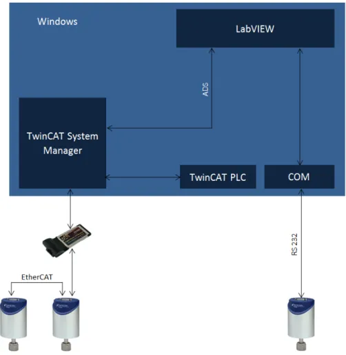
The graphic interface was developed to acquire the data from a specific measurement system. It is constituted by three different vacuum gauges that, in parallel, measure the pressure inside a vacuum pump, which may be increased or decreased by the user through a gas ballast valve, as shown in figure I.3.1.

(32)

One of the gauges communicates using the RS232 protocol, while the other two use the EtherCAT protocol. For the first case the computer is the master of the communication and is connected directly to the gauge using a COM port. In the second case the com-puter is also the master of the communication, however, it uses a 1 Gigabit Ethernet Lan ExpressCard as interface, since the Ethernet port is already used to connect to the Inficon’s network. The ports of the gauges and the adaptor are connected in a “daisy chain”, forming a small network with linear topology.

Due to the different sample rates of the two EtherCAT supporting gauges, a virtual PLC is also executed on the computer. It records the gauges data acting as an interface with the LabVIEW program, in order to guarantee synchronization and real-time accuracy. The EtherCAT virtual PLC (Programmable logic controller) and master are both config-ured with a real-time clock of 333 microseconds (3,003 kHz), ensuring that the Nyquist theorem is respected as the fastest gauge samples new data every 700 microseconds (1,428 kHz). These virtual devices are implemented by the TwinCAT (version 2.11.2220) tools, PLC Control and System Manager. TwinCAT stands for Windows Control and Au-tomation Technology and is a dedicated software from Beckhoff that turns computers with Windows NT/2000/XP/Vista/7/8 operating system into real-time controllers.

I.3.2. LabVIEW and TwinCAT data path implementation

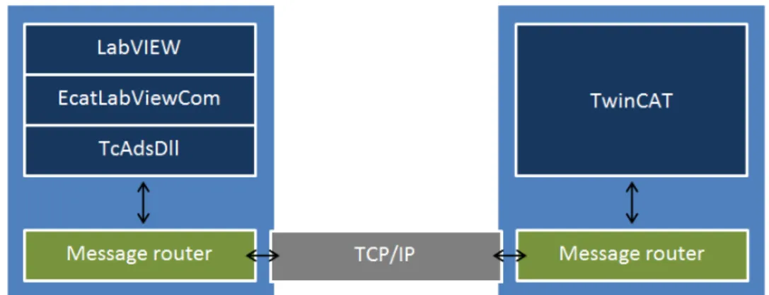
In order for process variables of the EtherCAT supporting gauges to be interpreted on the program created with LabVIEW a data path must be established between this one and the TwinCAT. The data exchange between these software programs is implemented by ADS (Automation Device Specification) interface.

The TwinCAT system architecture allows individual modules of the software (e.g. Twin-CAT PLC) to be treated as independent devices, and classified as “servers” or “clients” depending if they are acting like a hardware device or requiring the services from the “server”. The ADS interface lies on the exchange of messages between these objects by the "message router" over TCP/IP connections [11].

In the case of this project the TwinCAT is the server and LabVIEW could be classified as a client, which can implement directly the ADS communication by executing ADS-OCX methods, events and properties through Active X control elements. However, in

(33)

Chapter I.3 Methodology order to simplify the graphical programming, a dynamic-link library was developed, the

EcatLavViewCom, that is invoked by the LabVIEW program and implements all the

functions which require ADS interface, thus taking the client role. In turn, the ADS client methods are provided to the DLL by TcAdsDll from Beckhoff. In figure I.3.2, the scheme of the data path between LabVIEW and TwinCAT is shown.

Figure I.3.2.: Data path between LabVIEW and TwinCAT

I.3.3. Implementation

Considering the target measurement system and the data path between the graphic in-terface and the TwinCAT software, a set of three programs were developed: the PLC, the dynamic-link library and the LabVIEW client. They run in parallel as independent systems, although the communications between them are established hierarchically: the LabVIEW program is the master, which performs the data requests, the PLC is the slave, which receives the data from the measurement system and forwards it to the master, and the DLL is the interface between both. Throughout this chapter the pro-cesses implemented by these programs are described and the respective flowcharts are presented.

I.3.3.1. PLC programing

(34)

(35)

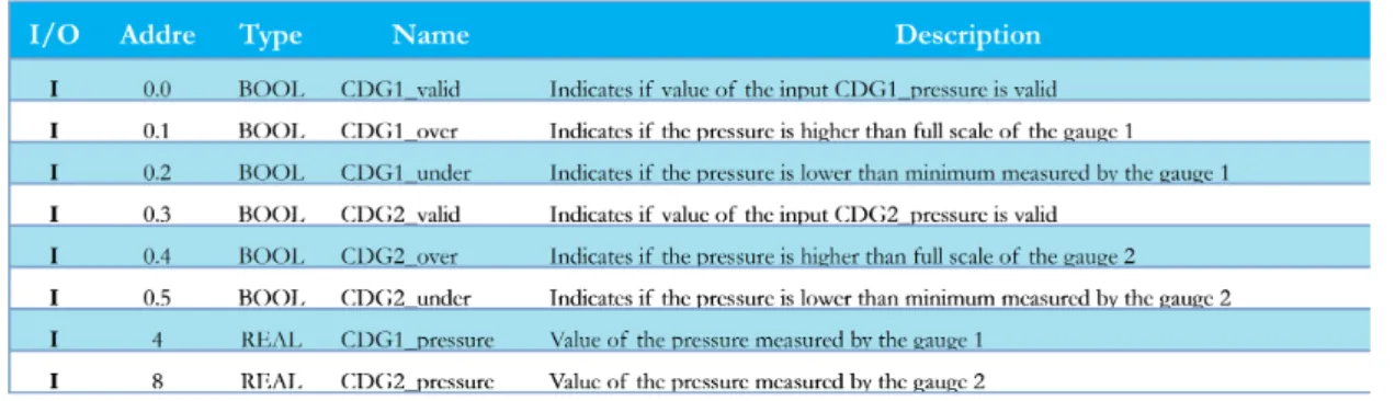
Chapter I.3 Methodology The PLC gets the measured pressure and three different information about its value: validity, overrange and underrange exceedance, from the two gauges. However, it has no outputs as the ADS interface allows the server variables to be read/written directly by the client. The PLC interfaces are shown in table I.3.1.

Table I.3.1.: Description of the PLC inputs/outputs

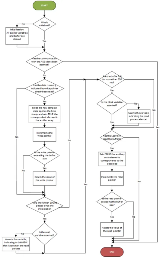
To ensure the synchronization of the data, safeguarding the real-time accuracy, the PLC applies a timestamp on every sampled data. The timestamp is a T_FILETIME struc-ture, a 64-bit value representing the number of 100 nanosecond intervals since 01/01/1601 00:00:00.00 (UTC). The Beckhoff TwinCAT has five different time sources. To perform the time stamping we use the TwinCAT/TC, a continuous TwinCAT clock initialized by Windows [12].

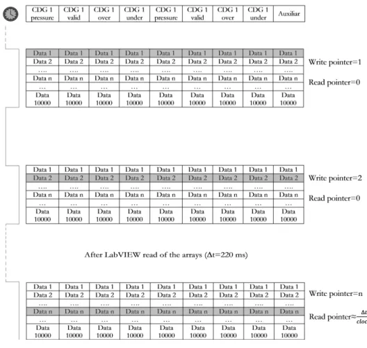
To avoid the loss of data due to the slow communication speed of the ADS interface (each polling function requires a 1-2 ms of protocol time [13]) the sampled data is saved in arrays of 10000 elements, which are read by the LabVIEW program every 220 mil-liseconds. These arrays behave as FIFOs and the access to them is controlled by an auxiliary binary array, with same length, and two distinct pointers. The elements of this auxiliary array are set to TRUE or FALSE depending if the FIFO element with correspondent index has valuable information or not, i.e. if it can be overwritten or not. For their turn, the write and read pointer save the values of the indexes subsequent to the latest written and read elements. The figure below (figure I.3.4) presents a graphic example of this control.

(36)

Figure I.3.4.: Example of the FIFOs access control

To guarantee that LabVIEW does not read empty buffers, a variable is asserted 100 milliseconds after the system initialization, enabling the ADS client to start the reading process. If after the start of the reading process the buffers are full with valuable data and LAbVIEW does not perform a reading cycle in a period of more than 300 millisec-onds another variable, indicating that reading process aborted, is asserted to protect the system from desynchronisation.

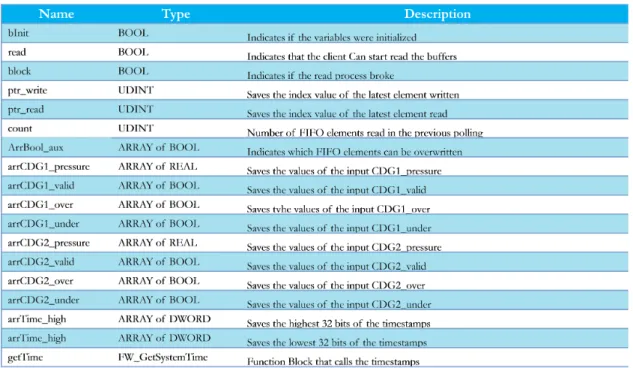
The PLC program used structured text as the programming language (Annex A.1) and is run cyclically at the clock rate indicated in section I.3.1. The complete set of varaibles used is summarized in table I.3.2.

(37)

Chapter I.3 Methodology

Table I.3.2.: Main variables of the PLC program

I.3.3.2. Dynamic-Link Library programing

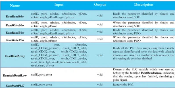
The dynamic-link library EcatLavViewCom program code, which can be consulted in Annex A.2, was developed in C++ language and complied by Visual Studio 2012. It implements seven different functions which require ADS interface. A resume of their inputs/outputs and description is presented in table I.3.3.

(38)

Table I.3.3.: Resume of all the functions of the DLL EcatLavViewCom

The functions which read/write the parameters through PDO services use the same ADS functions as the ones which use SDO services. The main difference between them lies in access addresses, i.e., in the ADS index group and index offset. These take the values of the parameter’s index and sub index, for the first case; while for the second case take the value of the Beckhoff global constant EC_ADS_IGRP_CANOPEN_SDO [14], in-dicating that the SDO service is used, and the result of the concatenation of the index and the subindex. The flowchart summarizing the process of these functions is presented in the figure I.3.5:

Figure I.3.5.: Flowchart of the functions which read/write EtherCAT parameters The function EcatReadArray reads all the data arrays from the EtherCAT virtual PLC and retrieves only the valuable data, i.e. the data that was not read in previous calls to the LabVIEW, and therefore responsible for establishing an interface between both programs. Due to its importance to the system synchronization it is also responsible for other management operations such as: assisting the PLC buffer control mechanism by retrieving the amount of valuable data saved; and asserting a acknowledge signal at the end of each cycle; and reinitializing the PLC in case of the reading process has been

(39)

Chapter I.3 Methodology aborted before. Figure I.3.6 shows the function program flowchart. All the parameters accessed in this function are PLC variables, thus is not possible to know their ADS addresses. Consequently, before the read/write operations a request is done using the name of the target variable, which returns the respective index and subindex.

(40)

As described in table I.3.3, the function EcatStartPLC is used to restart the PLC and the function EcatAckReadLow is used to deassert the variable which indicates the end of a reading cycle, immediatly after being asserted by the function EcatReadArray, reproducing a pulse signal. The flowcharts of both functions are shown in the figures below (figures I.3.7 and I.3.8):

Figure I.3.7.: Flowchart of the function EcatAckReadLow

Figure I.3.8.: Flowchart of the function EcatStartPLC

I.3.3.3. LabVIEW client programming

The main program was designed in a graphical programming language using LabVIEW 2012 Service Pack 1, version 12.0.1, as platform. It comprises a VI, which implements the main processes and the graphical user interface, and several subVIs. As shown in the Annex A.3, the program is divided in two sequences which execute the RS232 and EtherCAT related functions independently. To provide better system reliability and per-formance, all the functions in both sequences are run on different threads with distinct priorities, data acquisition and processing operations are faster than the screen updates and file storage, and thereby, have higher priority. The independency of the multiple threads is ensured by the use of queues in the transmission of data between functions. The main functions executed by the sequence related to the data coming from the RS232 gauge are: acquisition, file storage and screen update. The data acquisition function is implemented by a timed loop with a period of 1 millisecond, where the buffer of the COM port is analysed. When there are enough bytes to form a datagram (9 bytes), similar to the EtherCAT PLC program, a timestamp is applied to the data, ensuring its accuracy. The LabVIEW timestamp is a 128-bit data type that represents absolute time, the highest 64 bits represent the total seconds since the epoch 01/01/1904 00:00:00.00 UTC, while the lowest 64 bits represent the positive fraction of a second [16]. Between

(41)

Chapter I.3 Methodology two timestamps there may be a jitter, that in worst case is 20 milliseconds, which re-sults from the time period that the bytes arrive to the COM port (8 bytes at every 10 milliseconds). The 9 bytes datagram are decoded in a parallel thread by the subVI

ReadCDG_rs232, developed previously by Paul Wermelinger for the X-Chip Monitor

project [15].

The data is updated on the screen at a rate of 0.1 samples/ms and stored in file at rate defined by the user and multiple of 12 milliseconds. The file storage is configured by the subVI RS232SaveDataFile. The flowchart of the processes related to the data coming from the RS232 gauge is shown in the figure below (figure I.3.9).

(42)

(43)

Chapter I.3 Methodology

The other LabVIEW sequence implements the functions related to the data coming from the EtherCAT supporting gauges: data acquisition and processing, file storage, screen update and read/write of parameters using SDO services. These functions are only ex-ecuted after the PLC has been started and put in run mode. Figure I.3.10 shows the flowchart of these processes.

The data acquisition function is implemented by a timed loop with a period of 220 milliseconds which calls the functions EcatReadArray and EcatAckReadLow from the dynamic-link library EcatLavViewCom (see section I.4.2). The data retrieved from the PLC is then processed by the EtherCATDataDecoder subVI at a rate of 0.02 samples/ms, converting the C++ data types to suitable LabVIEW data types. The timestamp conversion is made in three steps: first the calculation of the num-ber of 100ns intervals as a double floating point numnum-ber by multiplying the high order uInt32 with 2^32-1 (4294967295.00) and then adding the low order 32bit value; second the subtraction the number of 100ns intervals between Jan 1, 1601 and Jan 1, 1904 (95’616’287’977’737’600.00), eliminating the offset between the two basetimes; and last division of the last result by 10’000’000 to get LabVIEW time. The data with the adapted data types is then updated on the screen at a rate of 2.1 samples/ms, and stored in file, at rate defined by the user and multiple of 333 micoseconds, using the subVI EtherCATSaveDataFile to configure the file and to control which samples are saved.

The several parameters available on the object dictionary of EtherCAT supporting gauges can be read/written using the CDGconfiguration subVI, which calls the func-tions EcatReadSdo or EcatWriteSdo, depending on the operation, from the

Ecat-LavViewCom DLL. Note that the IP address used on the ADS communications which

use SDO services is different from the ones which use PDOs, since in the CANopen devices are different for both cases. In the first case the CANopen device is TwinCAT, and therefore the IP address is the AMD netID of the computer running the program; in the second case the CANopen device is the network adaptor, the address being its netID.

(44)

Figure I.3.10.: Flowchart of the sequence implementing the functions related to the data provided by the EtherCAT gauges

(45)

I.4. Conclusions

This report has described the successful design and development of a graphical user in-terface which allows retrieving and processing data from standard vacuum gauges, using both the RS232 and the EtherCAT communication protocols, and from the new fast gauge just using the EtherCAT protocol.

To provide timely and accurate information from the new gauges with faster measure-ment rates, a particular attention was given to the real-time accuracy. One of the main difficulties that occurred at the implementation was the ADS communication speed of 1-2 ms, preventing LabVIEW to get the data directly using single ADS call at rate of 333 us. In the PLC other problem related to the real-time accuracy was encountered: the discharge time of the capacitors restrained the transmission speed, as for high fre-quencies a jitter was generated, causing some data losses. Another difficulty was the different data types used by LabVIEW and the dynamic-link library; several conversion functions were implemented to overcome this issue.

All the fundamental requirements were implemented with success, but some extra fea-tures could be added in the future to improve user experience, such as, error messages provided by the ADS functions to identify any problems that may happen in the net-work; and protections for the inputs, avoiding exceptions provoked by the user.

(46)

(47)

I.5. Zero Drift Compensation

I.5.1. Introduction

Capacitance diaphragm gauges, known as CDGs, are widely used in vacuum chambers to measure the pressure. Their performance is compromised by short and long term drifts, which are originated by unwanted bending of the diaphragm caused mainly by the pre-stress built into the sensor during manufacturing and the vacuum reference. However, a model of the drift is very difficult to obtain, since it is influenced by the geometry and material proprieties of each gauge.

The complex drift behavior prevents the use of simple compensation approaches and many investigations were performed in order to solve this problem. Dr. Peter Waegli developed a physical model and software application which fits and predicts the drift behavior; however it was proved inefficient for online compensation, as it needs several parameters barely accessible. In its turn Guintautas Mickus developed a prediction and compensation system using Inficon’s FabGuard, although its results were inconclusive. The main goal of this project is to continue the previous research focusing on long-term zero drift compensation using Kalman filters, as they proved to be very efficient for a wide range of applications.

I.5.2. Theoretical background

I.5.2.1. CDG measurement principle and zero-drift origins

Capacitance-diaphragm gauges with ceramic membranes have been on the market for about 15 years, being used for pressure measurement in a wide variety of applications, especially by the semiconductor industry, due to their high accuracy (typically 0.2 % of the measured value) and resistance against corrosive gases [17]. The measurement

(48)

principle lies on the deflection of a membrane under a differential pressure across it [18]. As shown in figure I.5.1, when a pressure (p) is applied the membrane suffers a deflec-tion (∆S ), changing the distance (∆d) between the two electrodes. This results in a capacitance variation (∆C ), which depends inversely on the applied pressure and can be used to determine it.

Figure I.5.1.: Measurement principle of the capacitance-diaphragm gauges The sensor output accuracy is compromised by zero drift, which can be classified in two different types depending on the time duration: term and long-term. The short-term drift occurs in the first days and according to Peter Waegli‘s research it is primarily influenced by the solder glass dimensions and elastic properties (G∞, τ and β), which control the bending of the membrane by glass shear. This shear can be simulated by the Burger Model, schematically shown in figure I.5.2, since the solder glass ring reacts to the pre-stess load analogous to an assembly of springs and dampers[19].

Figure I.5.2.: Shear of the glass solder simulated by the Burguer model [3] The maximum signal change observed in the long-term drift is controlled by the hous-ing dimensions and its mechanical properties (stiffness), and by the reference vacuum

(49)

Chapter I.5 Zero Drift Compensation pressure. One the other hand, it‘s time evolution is controled by the plastic properties of the solder glass (η), also known as the kinetic parameter [20].

I.5.2.2. Previous works

Previous research was done in order to diminish the effects of the zero drift. After set-tled a physical model for the drift, Peter Waegli developed a software application that fits and predicts the drift for SCS devices (mechanically similar to the CDG). However it proved to be inefficient as a routine tool since there are multiple optima fits due to the ambiguous behaviour of the drift and it is necessary to measure properties that are barely accessible by experiments with reasonable effort and/or the equipment at hand at Inficon[21].

As described in [17], Gintautas Mickus developed a system to model and compensate the zero drift. Two CDGs, one used to continuously measure the pressure in the cham-ber and other used periodically as reference, communicate with FabGuard, which in its turn, predicts and corrects the drift using trained models. The results suggested that it is possible to predict and train models in FabGuard for zero drift. However they were considered inconclusive since time was not tracked and several informations about the process in the chamber should have been considered, as process contamination also influences the drift behavior.

I.5.2.3. Kalman Filter

The drift behaviour depends on the geometry and material proprieties of the gauge. Therefore is very difficult to use simple correction techniques such as frequency analysis, baseline manipulation (removes the sensor response in the recovery cycle prior to sample delivery) or model temporal variations with a multiplicative correction factor [22]. In this project the performance of the Kalman filter is analysed as an online drift compen-sator, since it has low memory and computational requirements. This features make it suitable for implementation on a controller [23].

The Kalman filter is an optimal predictor-corrector type estimator that minimizes the estimated error covariance of dynamic systems which are affected by a certain random behavior [24]. As shown in the figure I.5.3, its algorithm can be divided in two distinct

(50)

phases: the time update, which “predicts” the present state (Xt) using information from the previous state (Xt-1); and the measurement update, which corrects the prediction using information from a new measurement. These phases are implemented recursively and embody a set of matrix equations, known as Riccati equations.

Figure I.5.3.: Algorith of the Kalman filter [21]

To apply the Kalman filter the model of the target system must be described by a state space form, i.e., by the measurement equation I.5.1, which describes the relationship between observed and unobserved variables, and a transition equation I.5.2 that describes the dynamics of the unobserved variables.

zk= H × xk+ vk (I.5.1)

xk+1= A × xk+ B × uk+ wk (I.5.2)

In these equations, wk and vk represent the state and measurement white noise with known covariance matrices Qk and R_k . Note that these two noises are statistically in-dependent. For some systems, the signal value xk+1can also be conditioned by a control

signal u_k. The entities A , B and H represent the state transition, input control and observation matrices.

(51)

Chapter I.5 Zero Drift Compensation

I.5.3. Kalman Drift

The data used to test the Kalman filter performance was gotten from Peter Waegli’s research. This data was collected by putting 10 different CDGs under zero pressure for 180 days in order to determine the zero drift caused by sensor cell’s manufacturing pre-stress and aging. As the focus of the project is the study of the long-term drift only the samples from the 60th to 180th day were used. The data acquisition and processing was performed by the Matlab function long-term-drift, developed in this project, which can be consulted in the Annex B.1.

Figure I.5.4.: Long-term drift

As shown in figure I.5.4, ignoring the low-frequency variations originated by the non-ideal conditions of the chamber, the drift of the several CDGs can be modeled as ramp signals. Being the slope the unknown variable, two state variables are needed: x1 is the signal and x2 is the slope. Considering that the input control is null and the measurement

noise is Gaussian, the CDG long-term zero drift can be modeled as shown in I.5.3.

x1 x2 ! k = 1 ∆t 0 1 ! × x1 x2 ! k−1 + 0 σ2 ! × w_k (I.5.3)

(52)

In this way, to predict and compensate the CDG long-term zero drift, a 1st order dis-crete Kalman filter was developed using the configuration presented in the table 3-1. A 2nd order discrete Kalman filter was also developed and its configuration is presented in the table I.5.1 as well. Both filters were implemented in Matlab, namely functions,

kalman_1st_order and kalman_2nd_order, whose codes can be consulted in the

Annexes B.2 and B.3.

Table I.5.1.: Configuration of the developed Kalman filters

I.5.4. Results and analysis

The outputs of the he 1st and 2nd order Kalman filters described in section I.5.3 are represented in figures I.5.5 and I.5.7. In order to diminish the drift effects Kamlan filter outputs were subtracted to the measured signals, obtaining the final results, which can be consulted in figures I.5.6 and I.5.8.

(53)

Figure I.5.5.: Output signals of the 1st order discrete Kalman filter

(54)

Figure I.5.7.: Output signals of the 2nd order discrete Kalman filter

Figure I.5.8.: Drift compensated signals and respective standard mean error

Figures I.5.5 and I.5.7 show that 2nd order filter has a slighter better performance than the 1st order filter, which was expected since the measured drifts are not linear due to low-frequency variations. Nevertheless, the corrected signals have practically the same error for both filters, as shown in the figures I.5.6 and I.5.8, proving that a higher order

(55)

Chapter I.5 Zero Drift Compensation discrete filter will not be more cost-effective.

As observed in figures I.5.5 and I.5.7, beside the low-frequency variations of the mea-sured signal that were caused by the non-ideal conditions of the chamber, the long-term zero drift has a linear tendency. And the figures I.5.6 and I.5.8 suggest that the Kalman filter could be used as drift compensator since all the corrected signals have an average more approximated to zero.

I.5.5. Conclusion

This report described the study of the Kalman filter as online drift compensator of the long-term zero drift, which compromises the accuracy of the Inficon’s gauges. Although the results from the experiment suggest that the Kalman filter can be used to predict and compensate the long-term zero drift„ this research should only be considered a starting point. Identified problems are discussed in the following paragraphs.

The Kalman filter precision is highly compromised by the precision of the system’s stochastic model, i.e, the model of the process and measurement noises. This experi-ment assumed noises characterized by ideal distributions (Gaussian) and variances; con-sequently to analyse the filter’s performance future researches should focus on the study of the system’s noises in order to develop a proper stochastic model of the longterm drift. The study carried out by Catherine Marselli [26] could be used as reference and start point for this matter.

The measured pressure signals exhibit some low-frequency variations caused by the non-ideal conditions of the chamber. As the present experiment assumed a simple approach and the pressure signal was considered as the drift signal, these variations were wrongly considered by the filter. In future experiments a threshold should be defined to distin-guish the variations of the gauge output signal caused by the variation of pressure inside the chamber from the drift.

(56)

(57)

References

[1] R. C. Dorf, “The Industrial Electronics Handbook Industrial Communication Sys-tems” 2011 , 2nd ed., B. M. Wilamowski and J. D. Irwinrs, Ed. Boca Raton: Taylor & Francis Group.

[2] Technical Introduction and Overview, EtherCAT Technology Group, Dcember 2004. [3] EtherCAT- the Ethernet FieldBus, EtherCAT Technology Group, November 2012. [4] M. Rostan, J. E. Stubbs and D. Dzilno, EtherCAT enbled Advanced Control Archi-tecture, 2010.

[5] M. Knezic, B. Dokic and Z. Ivanovic, “Topology Aspects in EtherCAT Networks”, in Proc. 14th International Power Electronics and Motion Control Conference, 2010. [6] G. Cena, I. C. Bertolotti, A. Valenzano and C. Zunino, A High-Performance CAN-like Arbitration Scheme for EtherCAT, Torino, Italy, 2009.

[7] J. C. Lee, S. J. Cho, Y. H. Jeon and J. W. Jeon, “Dynamic drift compensation for the Distributed Clock in EtherCAT”, in Proc. 2009 IEEE Internacional Conference on Robotics and Biomimetics, Guilin, China, December 2009.

[8] G. Cena, I. C. Bertolotti, A. Valenzano and C. Zunino, “On the Accuracy of the Distributed Clock Mechanism in EtherCAT”, Torino, Italy, 2010.

[9] EtherCAT Slave Controller IP Core for Xilinx FPGAs, Beckhoff Automation, 2009. [10] EtherCAT Slave Implementation Guide, EtherCAT Technology Group, October 2012.

[11] Beckhoff Information System. Accessed 20-11-2013. http://infosys.beckhoff.com/english.php? content=../content/1033/tcsample_labview/html/tcsample_labview_overview.htm&id=

[12] Beckhoff Information System. Accessed 20-11-2013. http://infosys.beckhoff.com/english.php? content=../content/1033/tcsample_labview/html/tcsample_labview_overview.htm&id=

[13] Beckhoff Information System. Accessed 20-11-2013. http://infosys.beckhoff.com/english.php? content=../content/1033/tcsample_vc/html/tcadsdll_api_cpp_sample17.htm&id=

[14] Beckhoff Information System. Accessed 20-11-2013. http://infosys.beckhoff.com/index.php?

content=../content/1031/tcplclib_tc2_ethercat/html/tcplclibtcethercat_globalvariables.htm&id=12401 [15] Paul Wermelinger. User Manual X-Chip Monitor. September 2012.

[16] Vacom. Total Pressure Measurement. In: Product Catalog 6th edition

[17] K. Jousten and S. Naef. On the stability of capacitandiaphragm gauges with ce-ramic membranes. AVS: Science & Technology of Materials, Interfaces, and Processing.

(58)

[18] Dr P. Waegli. Drift Issues with Membrane Type Pressure Sensors: final report on modelling of sensor behaviour and conclusions therefrom. Bremgarten, Switzerland. January 26, 2012.

[19] Dr P. Waegli. Selection Criterion: pre-stress, reference vacuum and measuring them. Bremgarten, Switzerland. May 30, 2012.

[20] Dr P. Waegli. Predicting Drifts of Membrane Type Pressure Sensors: summary report on drift-fit automation. Bremgarten, Switzerland. April 20, 2012. [6] National Instruments. Accesssed 20-11-2013. http://www.ni.com/white-paper/7900/en/

[21] Guintautas Mickus. CDG zero drift. July 26, 2013.

[22] R. Gutierrez-Osuna. Signal processing methods for drift compensation. 2nd NOSE II Workshop Linköping, 18 - 21 May 2003.

[23] M. J. Wenzel, A. Mensah-Brown, F. Josse and E. E. Yaz. Online Drift Compensa-tion for Chemical Sensors Using EstimaCompensa-tion Theory. IEEE Sensors Journal volume 11. January 2011

[24] G. Welch and G. Bishop. An Introduction to the Kalman Filter. University of North Carolina at Chapel Hill. August 12-17, 2001

[25] R. Jain and M. Epelbaum. Filtering Data. August 19, 2012. [12] Matlab Central. Accesssed 03-01-2014. http://www.mathworks.com/matlabcentral/fileexchange/16683-estimatenoise

[26] C. Marselli, D. Daudet, H. P. Amann, F. Pellandini. Application of Kalman filtering to noise reduction on microsensor signals. Proceedings of the Colloque interdisciplinaire en instrumentation,1998.

(59)

Part II.

(60)

(61)

II.1. Introduction

In the past decade, society has become highly dependent on the Internet and the number of users has grown at an exponential rate. While in 1994 less than 1% of world popula-tion had Internet access, today this number exceeds 40% [1]. This dependence became more pronounced with the introduction of several services such as Voice-over-IP (VoIP), Video on Demand (VoD) and Peer-to-Peer (P2P) file sharing. The traffic increase caused by these services, specially the ones involving multimedia content, compelled data cen-tres and carriers to upgrade their networks bandwidth up to 10/40 Gbps. This trend is challenging current Internet infrastructure, in particular the core routers, by demanding higher throughput and larger routing tables.

The router performance is mainly limited by the route lookup mechanism [2]. The objec-tive of IP lookup is to find the next hop to which send the packet, which is achieved by searching for the best match between the packet’s destination address and the entries in the routing table. To support the needs of current networks hardware-based routers are preferred to the traditional software-based routers. The last ones can not achieve high lookup rates, as a centralized CPU executes all functions, from control/management to data processing. In the hardware options, the field-programmable gate arrays (FPGAs) became an attractive choice, since their flexibility and reconfigurability allow the cre-ation of customized solutions. Also, the high resources available in these devices allows higher parallelism, increasing the throughput, as more data can be processed simultane-ously.

II.1.1. Objectives

Motivated by the problems outlined above, this project focuses on the study of IP lookup techniques and the development of an FPGA-based IPv4 router capable of handling data rates of 10Gbps. In order to achieve the proposed objectives, the activity plan presented in table II.1.1 was established.

(62)

Table II.1.1.: Activity Schedule

Activity February Marc

h

April Ma

y

June July

Study of IP Lookup Techniques X Study of Development Tools X

Design and Simulation X X X X X

Testing X X

Final Report X

The first phase involved the study of existing IP lookup techniques in order to find a mechanism that would be easily implementable in hardware and take few memory ac-cesses. Practical considerations such as cost were also an important concern.

In order to learn how to use the development tools HDL Designer, Quartus and Model-Sim, a simple project was designed, which consisted in changing a LED state (on/off ) at a frequency of 1Hz.

All the blocks necessary to preform the IP routing, were individually designed and sim-ulated during the third phase. A global system behaviour simulation was also carried out after all the blocks were validated. After having the system operating as desired, the project was compiled, loaded into the FPGA and real-time tested.

(63)

II.2. Fundamental Concepts

II.2.1. Ethernet

Ethernet is currently the most used Local Area Network (LAN) technology. Its standard comprises both the physical and the data link layers of the OSI model. The physical layer defines the speed (10Mbps up to 100Gbps), the medium and signal codification used in the transmission. The link layer is responsible for transmitting data between two adjacent hosts within the same LAN. It is generally divided into two sublayers: the Logic Link Control (LLC) and the Medium Access Control (MAC) [3].

The Logic Link Control sublayer is primarily concerned with providing services to the network layer. It encapsulates the higher-level packets into frames, allowing their trans-mission independently of the physical technology. The LLC can also provide flow and error control.

The Medium Access Control sublayer is responsible for the procedures used by the de-vices to access the network medium. Since Ethernet provides a medium shared by several hosts, the access medium is made according to the Carrier Sense Multiple Access With Collision Detection (CSMA/CD) scheme: before sending a frame the device must check if the medium is free and ready for a new transmission. When multiple devices send data at the same time collisions occur. The probability of a collision occurring increases with distance between hosts, due to the propagation delays of the electric signals. When a collision is detected the devices stop the transmission and send a jam signal, which is used to notify all the devices within the network about it. Only after some time, a host can try to resend the frame [3].

(64)

II.2.1.1. Frame Structure

An Ethernet frame starts following a 7-byte preamble and 1-byte start frame delimiter (SFD). The preamble comprises an alternate sequence of bits set to "0" and "1", and is used for bit synchronization. In its turn, the SFD is used for byte synchronization, as it is used by the receivers to detect the beginning of the frame.

The Ethernet frame structure has five fields, as shown in figure II.2.1. For 802.3 frames, the header has 14-bytes featuring the destination and source addresses, each with 6-byte length, and the EtherType field. The last one is 2-byte long, and if its value is superior to 1500 identifies which protocol is used in the payload. Otherwise, it represents the length of the payload. The payload must have a minimum length of 42 bytes, therefore a padding may be done. The Frame Check Sequence (FCS) is used to detect corrupted data within the entire frame by implementing a 4-byte cyclic redundancy check. (CRC) Ethernet devices must allow a minimum idle period between frames, which is known as interframe gap (IFG). The standard minimum IFG depends on the speed of the com-munication, for example, for 10 Mbit/s Ethernet the gap is 96 bits (12 bytes).

Figure II.2.1.: Ethernet Frame

II.2.1.2. Virtual LAN (VLAN)

Virtual LANs are widely used in today’s networks to improve performance and sup-port services, such as security. VLANs allow to change the network’s topology without changing the physical connection between hosts. A set of switches is used to construct network segments that behave logically like a conventional LAN but are independent of the physical locations of the hosts. In this way, data is only spammed between hosts within the same VLAN. To send data outside the VLAN a higher-level protocol, such as IP, must be used. In order to identify which VLAN a frame belongs to, a tag is inserted

(65)

Chapter II.2 Fundamental Concepts in the Ethernet header, as shown in figure II.2.2 [4].

Figure II.2.2.: VLAN Tag within Ethernet Frame

II.2.2. Internet Protocol Version 4 (IPv4)

The word Internet refers to the worldwide set of interconnected networks. These net-works are characterized by several different limitations, such as speed, number of users, maximum geographical distance and applicability to certain environments. The inter-operability between all the different networks that form the Internet is assured by the network layer protocol, IP (Internet Protocol). This protocol was designed primarily for inter networking; as a result it provides a best-effort routing service to deliver trans-mitted messages to their destination. Higher level applications must guarantee several functions such as reliability, flow control, or error recovery, since IP does not provide them. The first major version of IP, Internet Protocol Version 4 (IPv4), is currently the dominant protocol of the Internet [4].

II.2.2.1. Packet Structure

An IP packet is composed by the header section and the variable-length payload section. Typically, it is encapsulated in the data field of link layer frames, enabling the host to send data to any receiver, independently of the technology differences.

The IP header is formed by a 20-byte part and a variable-length optional part, ordered using big-endian convention. Therefore, the fields in the header are packed with the most significant byte to the left. The header format is shown in the figure II.2.3 and its fields are described below:

(66)

Figure II.2.3.: IPv4 Header Format

• The version field indicates which version of the protocol the packet belongs to. In the case of IPv4 it holds up the value 4.

• Since the header may contain a variable number of options, a second field, the

Internet Header Length (IHL), is provided to indicate the number of 32-bit words

in the header. The norm RFC 791 defines that the minimum value for this field is 5, which applies when no options are present. The maximum value is 15 as result of the 4-bit resolution.

• The Differentiated Services Code Point (DSCP) field, originally known as Type of

Service field, is defined by the norm RFC 2474 and classifies the packet according

to its type of service. In this way, a VoIP packet is distinguished from a text file packet, and both have a more suitable treatment during the routing process. • The Explicit Congestion Notification (ECN) field is an optional feature that allows

end-to-end notification of network congestion without dropping packets. It is only used when both endpoints support it and are willing to use it.

• The total number of bytes that compose the packet, including both header and data, are indicated by the Total Length field. Its minimum value corresponds to the minimum size of the header, which is 20 bytes. Being a 16-bit word, its maxi-mum value is 65,535 bytes.

• Sometimes restrictions on the packet size are imposed, in which case packets must be fragmented. In order to the host determine which packet a newly arrived frag-ment belongs to, the Identification field is used. Therefore, it contains the same

(67)

Chapter II.2 Fundamental Concepts value for all the fragments of a packet. Next follows a 3-bit field, which has also the purpose of control and identify the fragments. The position of a fragment in the packet is identified by the Fragment Offset field. Its value is measured in units of 8 octets (64 bits). The first fragment has offset zero.

• The Time to Live (TTL) is one of the essential fields for routing operations, as it indicates the maximum time the packet is allowed to remain in the Internet system. In practice, it counts hops: when the packet arrives at a router, the TTL value is decremented by one. When the TTL field hits zero, the router typically discards the packet and sends a warning packet back to the source host. This fea-ture prevents packets from wandering around indefinitely when the routing tables become corrupted.

• The Protocol field indicates which next level protocol (e.g. TCP, UDP) is used in the payload section of the packet. Each protocol has an assigned number that is global across the entire Internet. The list of IP protocol numbers is maintained by the Internet Assigned Numbers Authority.

• The IP header contains all the vital information, therefore it’s crucial to protect it against data corruption. The protection is achieved by the 16-bit Checksum field, which is calculated by the 16 bit one’s complement of the one’s complement sum of all 16 bit words in the header. At each hop the checksum is verified and the result should be zero if there is no corruption, otherwise the packet is discarded. Before sending the packet to the next hop the checksum is recalculated because at least one field always changes (the time to live field). In this case, the value of the checksum field is considered zero and is updated with the new value.

• The Source Address and Destination Address identify the network interfaces that belong to the sender and receiver.

• The Options field may appear or not in the packet. However, it must be im-plemented by all IP modules (host and gateways). It can be used for several applications such as security, route recording and time stamping. The field length is variable: there may be zero or more options, each being identified by a 1-byte code. Some options are followed by a 1-byte option length field, and then one or more data bytes. Zero padding is used to ensure that the header ends on a 32 bit