Improving minimum rate predictors algorithm for compression of volumetric medical images

DISSERTATION

Master in Electrical and Electronic Engineering

Improving Minimum Rate Predictors Algorithm for

Compression of Volumetric Medical Images

João Miguel Pereira da Silva Santos

DISSERTATION

Master in Electrical and Electronic Engineering

Improving Minimum Rate Predictors Algorithm for

Compression of Volumetric Medical Images

João Miguel Pereira da Silva Santos

Master dissertation performed under the guidance of Doctor Sérgio Manuel Maciel Faria, Professor at Escola Superior de Tecnologia e Gestão of Instituto Politécnico de Leiria and with the co-orientation of Doctor Nuno Miguel Morais Rodrigues, Professor at Escola Superior de Tecnologia e Gestão of Instituto Politécnico de Leiria.

If you can dream it, you can do it. (Walt Disney)

Acknowledgments

I would like to thank everyone that helped during this research work, and that made it possible to accomplish.

First to my advisers, Dr. Sérgio Faria and Dr. Nuno Rodrigues, that have chosen to introduce me to the research environment. I am thankful for their guidance and support that were essential for the proper development of this research. Also, I would like to thank their patience and availability to review my written works, both in papers and this dissertation. Their valuable insights helped improve the quality of this work.

This work was a part of the UDICMI project funded by CENTRO-07- ST24-FEDER-002022 of QREN and project Medicomp in the scope of R&D Unit 50008, financed by the applicable financial framework (FCT/MEC through national funds and when applicable co-funded by FEDER – PT2020 partnership agreement). I would like to thank to the members of these projects. Namely, Dr. Luís Cruz whose outside insights often helped to focus this work.

To Instituto de Telecomunicações and Escola Superior de Tecnologia e Gestão of Instituto Politécnico de Leiria for the excellent working conditions that certainly made this work much more productive. And to the local Multimedia Signal Processing group. Namely, André Guarda, Filipe Gama, Gilberto Jorge, João Carreira, Lino Ferreira, Luís Lucas, Ricardo Monteiro and Sylvain Marcelino. They made my time here much more enjoyable, with their friendship, great working environment and fruitful discussions. A special thanks must be given to Luís Lucas for his patience in Linux related questions and overall cluster management.

To all my friends, their patience and support during this time was amazing and helped me to focus on this work. A special mention is due to some of the friends I made at IPL. Namely, David Cruz, Hélder Simões, José Ricardo, Miguel Rasteiro and Ricardo Santos. We were always there for each other in the best and worse moments, and certainly have the memories to prove it.

To my family, their love and support were invaluable in the length of this work. They

Last but not the least, to Diana. Her unconditional friendship, love and patience are beyond everything I could possible expect. She always had the right words in the most difficult moments, even when this work did not allow us to be together as often as we would like.

Abstract

Medical imaging technologies are experiencing a growth in terms of usage and image resolution, namely in diagnostics systems that require a large set of images, like CT or MRI. Furthermore, legal restrictions impose that these scans must be archived for several years. These facts led to the increase of storage costs in medical image databases and institutions. Thus, a demand for more efficient compression tools, used for archiving and communication, is arising.

Currently, the DICOM standard, that makes recommendations for medical communi-cations and imaging compression, recommends lossless encoders such as JPEG, RLE, JPEG-LS and JPEG2000. However, none of these encoders include inter-slice prediction in their algorithms.

This dissertation presents the research work on medical image compression, using the MRP encoder. MRP is one of the most efficient lossless image compression algorithm. Several processing techniques are proposed to adapt the input medical images to the encoder characteristics. Two of these techniques, namely changing the alignment of slices for compression and a pixel-wise difference predictor, increased the compression efficiency of MRP, by up to 27.9%.

Inter-slice prediction support was also added to MRP, using uni and bi-directional tech-niques. Also, the pixel-wise difference predictor was added to the algorithm. Overall, the compression efficiency of MRP was improved by 46.1%. Thus, these techniques allow for compression ratio savings of 57.1%, compared to DICOM encoders, and 33.2%, compared to HEVC RExt Random Access. This makes MRP the most efficient of the encoders under study.

Keywords: DICOM, Lossless Compression, Medical Imaging, MRP.

Resumo

As tecnologias de imagens médicas têm vivido um crescimento, quer em termos do uso de imagens quer em termos de resolução das mesmas, nomeadamente em sistemas de diag-nóstico que requerem um grande conjunto de imagens, como a tomografia computorizada ou a ressonância magnética. Além disso, restrições legais impõem que este tipo de exames devam ser arquivados durante vários anos. Estes factos levam ao aumento dos custos de armazenamento em bases de dados ou instituições de imagens médicas. Portanto, existe uma necessidade crescente de ferramentas de compressão mais eficientes, usadas quer para armazenamento, quer para comunicação.

Atualmente, a norma DICOM, que faz recomendações para comunicações e compressão de imagens médicas, recomenda codificadores sem perdas, como o JPEG, RLE, JPEG-LS e JPEG2000. No entanto, nenhum destes codificadores inclui técnicas de predição inter-slice nos seus algoritmos.

Esta dissertação apresenta o trabalho de pesquisa efetuado sobre compressão de imagens médicas, usando o codificador MRP. O MRP é um dos algoritmos mais eficientes para compressão sem perdas de imagem. Inicialmente, são propostas várias técnicas de proces-samento para adaptar as imagens médicas às características do codificador. Duas destas técnicas (mudar o alinhamento das fatias para a compressão e o preditor de diferença pixel a pixel) aumentaram a eficiência da compressão do MRP até 27,9%.

Técnicas de predição inter-slice, tanto uni como bi-direccionais, foram desenvolvidas para o algoritmo MRP. Para além disso, o preditor de diferença pixel a pixel foi também adicionado ao algoritmo. Assim, a eficiência da compressão do MRP foi melhorada em 46,1%. Estas técnicas permitem ganhos na taxa de compressão de 57,1%, em comparação com os codificadores DICOM, e 33,2%, em comparação com o HEVC RExt Random Access. Estes resultados fazem do MRP o mais eficiente dos codificadores em estudo.

Palavras-chave: DICOM, Compressão sem Perdas, Imagens Médicas, MRP.

Contents

Acknowledgments iii

Abstract v

Resumo vii

Contents xi

List of Figures xiii

List of Tables xv

List of Abbreviations xix

1 Introduction 1

1.1 Context and motivation . . . 1

1.2 Objectives . . . 2

1.3 Dissertation structure . . . 3

2 Related State-of-the-Art 5 2.1 Medical imaging . . . 5

2.1.1 Computed Tomography . . . 6

2.1.2 Magnetic Resonance Imaging . . . 7

2.1.3 Image Dataset . . . 8

2.2 Digital imaging and communications in medicine . . . 9

2.3 Lossless coding algorithms . . . 10

2.3.1 A context based adaptive lossless image codec . . . 11

2.3.2 JPEG-LS . . . 12

2.3.3 JPEG2000 . . . 14

2.3.4 Multi-scale multidimensional parser . . . 16

2.3.5 3D-MMP . . . 17 ix

2.3.8 Minimum rate predictors . . . 22

2.4 Lossess codec comparison . . . 24

2.5 Other state-of-the-art techniques . . . 27

2.5.1 Scalable lossless compression based on global and local symmetries for 3D medical images . . . 27

2.5.2 Hierarchical oriented prediction for scalable compression of medical images . . . 30

2.5.3 Compression of X-ray angiography based on automatic segmentation 31 2.5.4 Progressive lossless compression . . . 32

2.5.5 Adaptive sequential prediction of multidimensional signals . . . 33

2.6 Summary . . . 34

3 Processing techniques for the compression of medical images 35 3.1 Concatenation of slices . . . 36

3.2 Directional approaches . . . 39

3.2.1 Slice formation on different axes . . . 39

3.2.2 Experimental tests . . . 40

3.2.3 Optimal compression plane algorithm . . . 43

3.3 Inter-slice prediction technique . . . 46

3.3.1 Pixel-wise difference predictor . . . 46

3.3.2 HEVC RExt Random Access prediction . . . 48

3.4 Prediction on different slice planes . . . 50

3.4.1 Pixel-wise difference calculated in different planes . . . 51

3.4.2 Pixel-wise difference compression in different planes . . . 52

3.5 Histogram packing . . . 53

3.6 Techniques comparison . . . 56

3.7 Summary . . . 58

4 Proposed Methods in Minimum Rate Predictors 59 4.1 Context calculation . . . 59

4.1.1 Experimental results . . . 60

4.2 Pixel-wise difference predictor . . . 61

4.3 Inter slice prediction . . . 62

4.3.1 Uni-directional prediction . . . 62

4.3.2 Bi-directional prediction . . . 63

4.3.3 Experimental Results . . . 65 x

4.3.4 Distance between slices . . . 71

4.4 Motion compensation . . . 74

4.4.1 Experimental results . . . 75

4.5 Optimal compression plane in MRP Video . . . 77

4.6 Contributions comparison . . . 78

4.6.1 Comparison with state-of-the-art lossless encoders . . . 79

4.7 Summary . . . 80

5 Conclusions 83 Bibliography 87 A Medical Sequences 95 B Histogram Packing Detailed Results 99 C Contributions 103 C.1 Published . . . 103

C.2 Submitted . . . 103

List of Figures

2.1 Sagittal slices of the brain by different imaging modalities. . . 6

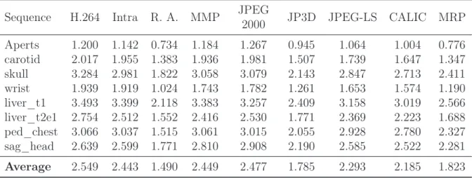
2.2 The principle of computed tomography with an X-ray source and detector unit rotating synchronously around the patient [31]. . . 7

2.3 MRI of the thorax [32]. . . 8

2.4 Middle slice of each of the used medical images [33]. . . 9

2.5 Schematic description of the CALIC coding system [8]. . . 11

2.6 Reference pixels positions. . . 12

2.7 JPEG-LS block diagram [4]. . . 13

2.8 Two-sided geometric distribution (TSGD) [4]. . . 14

2.9 General structure of JPEG-2000 [40]. . . 14

2.10 Wavelet transform decomposition for the skull sequence. . . 15

2.11 Code-block partitioning of a wavelet volume [11]. . . 16

2.12 Flexible block segmentation and partition tree [14]: (a) segmentation of an image block, (b) corresponding binary segmentation tree. . . 17

2.13 Triadic flexible partition [17]. . . 18

2.14 Block neighbourhood [17]. . . 18

2.15 Hierarchical video compression architecture [17]. . . 19

2.16 Basic coding structure of H.264 [19]. . . 19

2.17 H.264 intra prediction modes for 4 × 4 blocks [46]. . . 20

2.18 Basic coding structure of HEVC [22]. . . 21

2.19 HEVC intra prediction modes [22]. . . 21

2.20 Disposition of reference pixels [28]. . . 23

2.21 Example of the possible symmetries in medical images [48]. . . 28

2.22 Block diagram of the symmetry based scalable lossless compression tech-nique [49]. . . 30

2.23 Five proposed prediction modes for inter-slice DPCM prediction [49]. . . . 30

2.24 One prediction level of the HOP algorithm [2]. . . 31 xiii

3.1 Example of slice concatenation. . . 37

3.2 Slice orientation on a medical dataset. . . 39

3.3 Slice 101 of skull sequence for each plane. . . 40

3.4 Slice 51 of ped_chest sequence for each plane. . . 41

3.5 Example of the pixel-wise difference predictor. . . 46

3.6 Example of the residue obtained for the skull sequence for slice 29. . . 50

4.1 Reference pixels in the previous slice. . . 63

4.2 Usual bidirectional prediction dependencies . . . 64

4.3 HEVC bidirectional prediction scheme [22]. . . 64

4.4 Motion compensation example [65]. . . 74

A.1 Slices of the CT Aperts sequence [33]. . . 95

A.2 Slices of the CT carotid sequence [33]. . . 95

A.3 Slices of the CT skull sequence [33]. . . 96

A.4 Slices of the CT wrist sequence [33]. . . 96

A.5 Slices of the MR liver_t1 sequence [33]. . . 96

A.6 Slices of the MR liver_t2e1 sequence [33]. . . 97

A.7 Slices of the MR ped_chest sequence [33]. . . 97

A.8 Slices of the MR sag_head sequence [33]. . . 97

List of Tables

2.1 Description of the used medical images datasets. . . 8

2.2 Prediction value for the pixel given by GAP. . . 12

2.3 Performance comparison of the image encoders (results in bpp). . . 26

2.4 Performance comparison of the video encoders (results in bpp). . . 26

2.5 Compression results of the 3D-MMP (results in bpp). . . 27

2.6 Spatial transformations [48]. . . 29

3.1 Number of slices used by each processing techniques. . . 35

3.2 Coding performance evaluation for lossless encoders using the number of slices given in Table 3.1 (results in bpp). . . 36

3.3 Compression results of the concatenated slices (in bpp). . . 37

3.4 Percentage of improvement on coding performance when using concate-nated slices (in %). . . 38

3.5 Compression results for slices aligned with the YZ plane (in bpp). . . 41

3.6 Percentage of compression gain when changing the plane direction from XY to YZ. . . 42

3.7 Compression results for slices aligned with the XZ plane (in bpp). . . 42

3.8 Percentage of compression gain when changing the plane direction from XY to XZ. . . 42

3.9 Correlation coefficients for all directions and choice of the best OCP. . . . 44

3.10 Intra compression results using OCP algorithm (in bpp). . . 45

3.11 Percentage of compression gain when using OCP algorithm, compared to the compression in YZ plane aligned slices. . . 45

3.12 Results of the encoding of the pixel-wise difference residue (in bpp). . . 47

3.13 Percentage of compression gain when using the pixel-wise difference predictor. 47 3.14 Number of lossy pixels of the HEVC RExt residual. . . 49

3.15 Results of the encoding of the HEVC RExt residue (in bpp). . . 49

3.16 Percentage of compression gain when using the HEVC RExt residue, com-pared to the pixel-wise difference predictor. . . 49

3.18 Coding performance for the pixel-wise difference applied on the YZ plane (results in bpp). . . 51 3.19 Coding performance for the pixel-wise difference applied on the XZ plane

(results in bpp). . . 52 3.20 Coding performance for pixel-wise difference in the YZ plane (results in bpp). 53 3.21 Coding performance for the pixel-wise difference in the XZ plane (results

in bpp). . . 53 3.22 Results of the use of histogram packing before the encoding (in bpp). . . . 54 3.23 Percentage of compression gain when using the histogram packing. . . 54 3.24 Average number of actual values present in the medical sequences. . . 55 3.25 Average number of values actually present in the medical images from [61]. 55 3.26 Average compression results for images from [61], with and without

his-togram packing, using JPEG-LS (results in bpp). . . 56 3.27 Comparison of the techniques applied to HEVC RExt Random Access

(re-sults in bpp). . . 57 3.28 Comparison of the techniques applied to MRP (results in bpp). . . 57 4.1 Comparison between the original MRP algorithm context and the proposed

context calculation (results in bpp). . . 60 4.2 Number of lossy pixels in a sequence when using the pixel-wise difference

predictor and its transmission cost. . . 61 4.3 Optimisation of the K1 and K2 parameters for each sequence. . . 66

4.4 Compression results of the optimised K1 and K2 parameters (in bpp). . . . 66

4.5 Optimisation of the K1 and K2 parameters for each sequence, using

pixel-wise difference predictor. . . 67 4.6 Compression results of the optimised K1 and K2 parameters, using

pixel-wise difference predictor (in bpp). . . 67 4.7 Optimisation of the K1, K2 and B parameters for each sequence, using

MPEG-2 B-type slices. . . 68 4.8 Optimisation of the K1, K2 and B parameters for each sequence, using

HEVC B-type slices. . . 68 4.9 Compression results of the optimization of the K1, K2 and B parameters

for the MPEG-2 B-type slices (in bpp). . . 69 4.10 Compression results of the optimization of the K1, K2 and B parameters

for HEVC B-type slices (in bpp). . . 69 xvi

4.11 Optimisation of the K3and K4 parameters for each sequence, using

MPEG-2 B-type slices. . . 70 4.12 Optimisation of the K3 and K4 parameters for each sequence, using HEVC

B-type slices. . . 70 4.13 Compression results of the optimization of the K3 and K4 parameters for

the MPEG-2 B-type slices (in bpp). . . 71 4.14 Compression results of the optimization of the K3 and K4 parameters for

HEVC B-type slices (in bpp). . . 71 4.15 Optimization of the parameter D for uni-directional prediction (results in

bpp). . . 72 4.16 Optimization of the parameter D for uni-directional prediction, using

pixel-wise difference predictor (results in bpp). . . 72 4.17 Optimization of the parameter D for MPEG-2 bi-directional prediction

(results in bpp). . . 73 4.18 Optimization of the parameter D for HEVC bi-directional prediction

(re-sults in bpp). . . 73 4.19 Motion compensation compression results for natural sequences (in bpp). . 75 4.20 In-loop motion compensation compression results for natural sequences (in

bpp). . . 76 4.21 Percentage of compression efficiency difference between the proposed

mo-tion compensamo-tion and the results of [67]. . . 76 4.22 Percentage of compression efficiency difference between the proposed

in-loop motion compensation and the results of [67]. . . 76 4.23 Compression results for inter-slice prediction using OCP (in bpp). . . 78 4.24 Optimal parameters used in the various types of inter-slice prediction. . . . 78 4.25 Comparison of the improvements made to MRP (results in bpp). . . 79 4.26 Percentage of compression efficiency gains of the MRP proposed

improve-ments. . . 79 4.27 Comparison of the proposed alterations to MRP with the original encoder

and HEVC RExt (results in bpp). . . 80 B.1 Number of values actually present in the medical images from [61]. . . 99 B.2 Compression results for images from [61], with and without histogram

pack-ing, using JPEG-LS (results in bpp). . . 100

List of Abbreviations

2D: Two Dimensional, p. 9 3D: Three Dimensional, p. 15 bpp: bits-per-pixel, p. 25

CALIC: Context based Adaptive Lossless Image Codec, p. 2 CC: Correlation Coefficient, p. 43

CIPR: Center for Image Processing Research, p. 8 CR: Computed Radiography, p. 55

CT: Computed Tomography, p. 1 CTU: Coding Tree Unit, p. 21

DCT: Discrete Cosine Transform, p. 20

DICOM: Digital Imaging and Communications in Medicine, p. 1 DPCM: Differential Pulse Code Modulation, p. 17

DWT: Discrete Wavelet Transform, p. 15

EBCOT: Embedded Block Coder with Optimized Truncation, p. 16 GAP: Gradient-Adjusted Predictor, p. 11

HEVC: High Efficiency Video Coding, p. 2 HEVC RA: HEVC Random Access, p. 25 HEVC RExt: HEVC Range Extension, p. 22

HOP: Hierarchical Oriented Prediction, p. 30

ISO: International Organization for Standardization, p. 9 ITU: International Telecommunication Union, p. 9

JP3D: JPEG2000 Part 10, p. 2

JPEG: Joint Photographic Experts Group, p. 2

JPEG-LS: Lossless and near-lossless compression of continuous-tone still images, p. 2

Least Squares Prediction, p. 17 MDL: Minimum Description Length, p. 33 MED: Median Edge Detector, p. 13

MMP: Multi-scale Multidimensional Parser, p. 2 MPEG: Motion Picture Experts Group, p. 63 MRI: Magnetic Resonance Imaging, p. 1 MRP: Minimum Rate Predictors, p. 2 OCP: Optimal Compression Plane, p. 43 RLE: Run Length Encoding, p. 2

ROI: Region of Interest, p. 27

TSGD: Two-Sided Geometric Distribution, p. 13

US: Ultrasound, p. 1

VBS: Variable Block Size, p. 22

Chapter 1

Introduction

1.1

Context and motivation

Since medical imaging was first used for diagnostics purposes it has been an ever expanding field. The need for better medical diagnosis has driven the medical imaging technologies in the last decades. The expansion in this technology has led to an increasing demand for the use of such diagnostic tools, revolutionising the practice of medicine.

Concurrently, the advance in technology has led not only to new medical imaging tech-nologies, but also to better image quality in several imaging types. Therefore, currently medical images have higher resolution and bit depths. Nowadays, resolutions of 512 × 512 pixels are considered to be the minimum, although most recent scanning systems are able to capture slices with spatial resolutions up to 1024 × 1024 pixels. Also, in such exams as Computed Tomography (CT), Magnetic Resonance Imaging (MRI) or Ultra-sound (US), that are comprised by several slices, thin-slice scanning techniques have been arising. Thus, leading to the increase of the number of slices in volumetric sequences, as the inter-slice resolution has improved from typically 5mm to 0.6mm over the years [1]. Due to medical and legal reasons [2] the results of these scans need to be kept and archived for several years. Moreover, the archiving process needs to guarantee that the scans are kept in same state as during the diagnosing process. This is relevant, for instance, for cases where judicial proceedings due to medical malpractice, or others, might arise, but also for patient record keeping.

Consequently, medical images archiving databases are facing a quasi-exponential growth in their contents [2]. Therefore, a new field in medical imaging compression has emerged, in order to efficiently archive and transmit the ever growing medical imaging databases information. Currently, Digital Imaging and Communications in Medicine (DICOM), the

organism that makes recommendations for medical communications and imaging archiv-ing, recommends lossless encoders such as JPEG, Run Length Encoding (RLE), Loss-less and near-lossLoss-less compression of continuous-tone still images (JPEG-LS) [3, 4] and JPEG2000 [5–7] for this purpose.

Although, these are the currently recommended encoders for medical imaging compression there are several other state-of-the-art lossless encoders. These encoders show higher com-pression efficiency rates than the ones proposed by DICOM. Some of these encoders were used in this work, namely: Context based Adaptive Lossless Image Codec (CALIC) [8,9], JPEG2000 Part 10 (JP3D) [10–12], Multi-scale Multidimensional Parser (MMP) [13–16], 3D-MMP [15,17], H.264 [18–20], High Efficiency Video Coding (HEVC) [21–23] and Min-imum Rate Predictors (MRP) [24–28] encoder. MRP was the focus of this research, due to having one of the highest lossless compression efficiencies for still images [16]. In this work a comparison between these encoders applied to medical images is performed. All DICOM recommended lossless encoders fail to exploit inter-slice redundancy in med-ical volumetric datasets. Considering this, and the fact that MRP has a high lossless compression efficiency for continuous-tone still images, in this work we propose to add inter-slice prediction support to this encoder.

The experimental results show that the MRP encoder achieves the highest compression efficiency performance for the used medical datasets for the considered encoders. These results show that this encoder is a good candidate for standardisation in the DICOM scope.

1.2

Objectives

The main topic of this research was to develop more efficient techniques to improve the reversible compression of medical images. As one of the most efficient state-of-the-art lossless encoders for the compression of continuous-tone images the MRP algorithm was chosen as a starting point to this work. Therefore, the following topics were developed:

• Study and comparison of state-of-the art lossless encoders present in the literature, when applied to medical image compression.

• Development of techniques to improve the compression efficiency of medical images by exploiting the characteristics of the images and of the lossless encoders, namely MRP.

• Extension and improvement of the MRP algorithm for the compression of medical images, by adding inter-slice prediction support to the encoder.

1.3. Dissertation structure 3

1.3

Dissertation structure

This dissertation is organized in five chapters and three appendixes. This chapter intro-duces this research work through its context, motivation and objectives.

Chapter 2 is dedicated to the state-of-the-art analysis relevant to this research work. Ini-tially, medical imaging technologies, focusing in CT and MRI, and the DICOM standard are described. Then, a brief summary of the used lossless encoder algorithms is given, with a full description of MRP, and their compression efficiency is compared. The chapter is concluded with a review of some relevant state-of-the-art works.

In Chapter 3, processing techniques are proposed to enhance the compression efficiency of the MRP algorithm. This chapter focuses on techniques applied prior to the compression process in the encoder algorithms. Chapter 4, describes the proposed techniques added to the MRP algorithm, as well as the compression efficiency provided by those contributions. The chapter is concluded with a comparison of these proposed contributions. Chapter 5 draws some conclusions on the work presented in this dissertation and presents suggestions for future work in this field.

Appendix A, exhibits the medical images used in the experiments throughout this work. Appendix B, shows more detailed results of tables present in Section 3.5 of Chapter 3. Finally, in Appendix C a list of published and submitted papers, that resulted of this research work, is provided.

Chapter 2

Related State-of-the-Art

In this chapter the current state-of-the-art on medical images compression will be pre-sented and discussed. We will start by giving a brief overview on medical imaging tech-nologies, focusing on the used medical sequence types. Then we will proceed to describe the DICOM standard and the lossless encoders that are used in this research. Finally, re-cent developments in the field of lossless compression, both of continuous-tone and medical images, will be described.

2.1

Medical imaging

Medical imaging emerged with the increasing comprehension of several physical phenom-ena. Recent advances in understanding and use of these phenomena, such as X-ray, γ-ray, ultrasound waves and positron emission production, propagation and recording are strongly linked to the progress in different fields of medical imaging technologies. The availability of digital acquisition technologies and powerful computational resources are also driving new developments and useful solutions, e.g., tomography reconstruction both static and time-varying, etc.

There are several types of medical imaging modalities, for example Computed Tomog-raphy (CT), Magnetic Resonance Imaging (MRI), Ultrasound (US) imaging, Positron Emission Tomography, Elastography, etc. Each of these modalities have their own charac-teristics [29,30], that depend on the associated physical processes and acquisition methods. Figure 2.1 shows four sagittal slices of a brain acquired with different technologies, where the distinguishable characteristics of various imaging modalities are clearly observable. The characteristics of each medical imaging modality are also dependent on the domain of application. Thus, studies are necessary to assess where, when and how each type of image

Figure 2.1: Sagittal slices of the brain by different imaging modalities. From top-left to down-right: Magnetic Resonance Imaging, Computed Tomography, Positron Emission Tomography and Ultrasound [29].

can be adequately used. For instance, X-rays are more adequate to image bone structures, while Magnetic Resonance provide higher definition and represents more accurately the softer tissues. In this work, we will focus on two of the most common volumetric medical imaging types, CT [30, 31] and MRI [30, 32] scans.

2.1.1

Computed Tomography

Computed Tomography (CT) has been used since the mid-1970’s when it introduced a revolution in medical imaging [31]. Nowadays, millions of scans are performed around the world. A CT scanner consists of a ring housing a rotating X-ray source and a axially opposed corresponding detector, as depicted in Figure 2.2. The body is stationary inside the ring, and thousands of images are taken while the source-detector assembly rotates around the ring axis. If the body is moved longitudinally then a set of scans can be acquired to produce a CT volume.

CT scans can produce more detailed images than those of traditional X-rays, especially for the internal organs. The physical process behind computed tomography is the atten-uation of X-rays in the body, where the amount of radiation absorption depends on the characteristics of the tissues in the path of the X-rays, so that different tissues will lead to different intensity readings by the detector [30].

2.1. Medical imaging 7

Figure 2.2: The principle of computed tomography with an X-ray source and detector unit rotating synchronously around the patient [31].

One of the advantages of CT is the speed of a complete scan, typically on the order of seconds or less. With the addition of a contrast agent further studies in blood vessels and organs can be made, but the preferred domain of application of CT is in bones imaging. Due to its capture speed, CT imaging is very valuable in emergencies and have an im-portant role in the diagnosing strokes, brain injuries, and others. Despite this, a CT scan exposes the body to more radiation than a conventional X-ray, and so CT are not recommended to some patients, such as pregnant women, or for repeated use.

2.1.2

Magnetic Resonance Imaging

Magnetic Resonance Imaging (MRI) uses magnetic fields and radio-frequency pulses, in order to obtain images of the internal structures from the human body. MRI scanners produce high contrast and very detailed images of the soft tissues and internal organs structure, for instance the brain, as can be seen in Figure 2.3 [32].

MRI scans are used in various examinations, such as brain exploration, detection of tu-mours or assessing the blood flow in different organs. MRI have the advantage of being able to reproduce high quality and high contrast images of the human body, without the need for contrast agents or the use of harmful radiations. The disadvantage of MRI is that patients with metallic implants or pacemakers might be put at risk by the magnetic fields that are involved in the imaging process.

An MRI system makes use of a magnet that creates a static magnetic field and which is "focused" on a specific body part. The signal is switched on and off, and the reflected radio-waves are processed to compute the absorption and reflection of these waves [30]. This information is used to render images with a direct correspondence to the physical

Figure 2.3: MRI of the thorax [32].

characteristics and location of the tissues.

MRI scanners can be used for a wide range of body parts including injuries of the joints, blood vessels, breasts, as well as abdominal and pelvic organs such as the liver or repro-ductive organs. Many diseases, such as brain tumours, can be visualized using this type of images because of the high contrast definition.

2.1.3

Image Dataset

The image dataset used to assess the performance of the encoders during this research is composed of eight volumetric medical sequences: four CT and four MRI scans, all available in [33]. These images are available on the repository of the Center for Image Processing Research (CIPR) of the Rensselaer Polytechnic Institute. The spatial resolution, bit depth and number of slices of each volume are shown in Table 2.1.

Table 2.1: Description of the used medical images datasets. Datasets Type Slices Resolution Bits-per-pixel Aperts CT 97 256 × 256 8 carotid 74 256 × 256 8 skull 203 256 × 256 8 wrist 183 256 × 256 8 liver_t1 MRI 58 256 × 256 8 liver_t2e1 58 256 × 256 8 ped_chest 77 256 × 256 8 sag_head 58 256 × 256 8

2.2. Digital imaging and communications in medicine 9

These data volumes are sets of spatially adjacent slices that require a large number of bits to be represented, due to their resolution and number of slices, as well as bit depth. Fig-ure 2.4 shows only the midpoint slice of each volume of the dataset, which are completely shown in Appendix A.

(a) CT Aperts (b) CT carotid (c) CT skull (d) CT wrist

(e) MRI liver_t1 (f) MRI liver_t2e1 (g) MRI ped_chest (h) MRI sag_head

Figure 2.4: Middle slice of each of the used medical images [33].

2.2

Digital imaging and communications in medicine

Digital Imaging and Communications in Medicine (DICOM) [5–7] is an international standard for compression, communications and related information of medical images, first published in 1993. This standard is present in most of the medical imaging devices, such as CT, MRI, etc., being the most widespread healthcare standard in the world. The use of standards is particularly essential in medical imaging [30], as it assures that images can be interchangeably used and shared between the various institutions, hospitals, imaging centres, etc.

The DICOM standard is mainly a protocol for image exchange. In the context of this particular work, we are interested in its specifications for image compression. In the standard, an image data is defined as a simple Two Dimensional (2D) representation of values in a series or dataset. With the growing needs of US, CT and MRI imaging, a multi-slice concept was designed [30].

DICOM integrates common image compression standards, both reversible (lossless) and irreversible (lossy), from International Organization for Standardization (ISO) and

Inter-national Telecommunication Union (ITU). The standard defines an encapsulated format archive, where the compression information is included in the bit-stream syntax [34]. Despite allowing a number of coding algorithms to be used, the standard makes no as-sumptions or recommendations on which encoders should be applied and in which appli-cations [6].

This is especially valid for the irreversible encoders, as there is still an open debate on whether lossy compression should be used in the context of medical imaging, specially when images are used for diagnose purposes. Regulatory bodies in the UK, EU, USA, Canada and Australia allow the use of lossy compression for medical images. However, the decision of using irreversible compression is left for the institutions and radiologists [35]. Despite this, reversible compression is recommended by several regulatory bodies, such as the Royal Australian and New Zealand College of Radiologists, where possible [36]. The DICOM standard supported encoders are the following:

• JPEG, for lossy and lossless compression; • RLE, for lossless compression;

• JPEG-LS, for near-lossless and lossless compression; • JPEG2000, for lossy and lossless compression;

• MPEG-2, for image compression using the main profile and the main or high levels, for lossy compression;

• H.264, for video compression using the main and the stereo main profiles, levels 4.1 or 4.2, for lossy compression.

As can be seen, there are no video lossless encoders contemplated in the DICOM standard. In this research work, the lossless encoders allowed in the standard and state-of-the-art lossless encoders were also studied and compared. This work focus on the compression of medical sequences, such as CT and MRI, therefore the inter-slice prediction and lossless video compression was also addressed.

2.3

Lossless coding algorithms

In this section current DICOM and state-of-art lossless encoders are described. It is expected that the compression algorithms will be better understood and, therefore, allow us to better exploit their characteristics. This work is mainly focused on the Minimum Rate Predictors (MRP) encoding algorithm, thus, it is fully described.

2.3. Lossless coding algorithms 11

2.3.1

A context based adaptive lossless image codec

Context based Adaptive Lossless Image Codec (CALIC) [9] is a lossless image encoder for continuous-tone images. CALIC started as a candidate algorithm to ISO/JPEG stan-dardisation, aimed to lossless encoding of continuous-tone images [8]. Eventually, CALIC was passed over, and the LOw COmplexity LOssless COmpression for Images (LOCO-I)1

algorithm was chosen, despite being more efficient, but presenting higher computational complexity.

The encoding and decoding process works in a raster scan order, requiring only a sin-gle pass. The prediction requires only values from the two previous lines of the image. Figure 2.5 shows a block diagram for the CALIC algorithm.

Binary mode? Context Generation & Quan-tization Ternary Entropy Coder Conditional Proba-bilities Estimation Two-row Double Buffer Gradient-adjusted Prediction + − Error modelling Coding Histogram Sharpening Entropy Coder I yes no ε Ï İ -_ε code stream

Figure 2.5: Schematic description of the CALIC coding system [8].

CALIC uses a two step approach, prediction followed by context modelling for the resid-ual coding. This encoder utilizes a context-based predictor in order to efficiently model the image data and characteristics. CALIC has two distinct operation modes, binary and continuous tone, the choice between these two modes is automatically made in the com-pression process. The binary mode is used when a given area of the image has just two distinct intensity values, and the symbols are encoded with a ternary entropy coder. In the continuous mode, a set of prediction, context modelling and entropy coding is used. For the prediction step, a simple gradient-based non-linear prediction scheme, Gradient-Adjusted Predictor (GAP), is used. The GAP prediction adjusts its coefficients based on

1

This algorithm and the resulting standard led to the JPEG-LS encoder. This encoder will be described in the next section.

local gradients estimation. This predictor is context sensitive and adaptable by modelling of prediction errors and feedback from the expected error, conditioned by properly chosen modelling contexts, as can be seen in Figure 2.5. The performance of the GAP predictor is improved via context modelling. Figure 2.6 shows the possible reference pixels, in black, relative to the current pixel x, in red. The local gradients are determined as in Equation 2.1, and Table 2.2 shows the prediction result, according to the gradients. The prediction errors of the continuous mode are then encoded using an adaptive m-ary arithmetic encoder, CACM++ [37].

nn nne

nw n ne

ww w x

Figure 2.6: Reference pixels positions.

dh = |w − ww| + |n − nw| + |ne − n|

dv = |w − nw| + |n − nn| + |ne − nne|

(2.1)

Table 2.2: Prediction value for the pixel given by GAP. Edge type Horizontal Vertical

Sharp w n Normal aux+ w 2 aux+ n 2 Weak 3 × aux + w 4 3 × aux + n 4 aux= w+ n 2 + ne− nw 4

2.3.2

JPEG-LS

Lossless and near-lossless compression of continuous-tone still images (JPEG-LS) [3,4], not to be confused with the lossless version of the JPEG encoder, is a JPEG, ISO/ITU stan-dard for lossless and near-lossless compression of continuous-tone images. This encoder is based on the LOw COmplexity LOssless COmpression for Images (LOCO-I) algorithm. This algorithm is divided into three main stages, prediction, context modelling and residue coding, as represented in the block diagram of Figure 2.7.

2.3. Lossless coding algorithms 13

Figure 2.7: JPEG-LS block diagram [4].

The JPEG-LS prediction uses the template depicted on the left side of Figure 2.7. In this template, a, b, c and d are neighbouring samples of the current sample x. This template is on the causal area of the image and, by using only four past samples, JPEG-LS limits the image buffering requirements.

A fixed prediction scheme given by Equation 2.2 is used in the encoder. This predictor tends to pick pixel b when a vertical edge is present, pixel a when a horizontal edge is detected and a + b − c if no edge is present. This predictor is called Median Edge Detector (MED). ˆ x ,          min(a, b), if c ≥ max(a, b) max(a, b), if c ≤ min(a, b) a+ b − c, otherwise. (2.2)

After the prediction stage, a context modelling is applied to the prediction error. In LOCO-I a Two-Sided Geometric Distribution (TSGD) model is used for the modelling, as the example showed in Figure 2.8.

The context that shapes the current prediction residual encoding is determined from the local gradient surrounding the current sample. Therefore, the level of activity can be determined, which in turn allows for the determination of the statistical behaviour of the prediction errors.

Finally, to encode the prediction residual errors, JPEG-LS uses a minimal complexity subfamily of the optimal prefix codes for TSGDs. These optimal codes are based on Golomb codes [38], which allow the calculation of the code word for any given sample without the use of code tables. This encoding method is adaptive; when a new sample is encoded the contexts and the probabilities are updated in order to further optimize the

Figure 2.8: Two-sided geometric distribution (TSGD) [4].

encoding process.

2.3.3

JPEG2000

JPEG2000 [39, 40] is a standard for image compression, maintained by ISO/IEC 15444-1 and ITU recommendation T.815444-12. JPEG2000 is a wavelet transform based encoder with applications from natural images to medical imaging and others. This standard has essentially been established to be a more efficient encoder and substitute to the JPEG encoder. The general structure of the JPEG2000 codec is shown in Figure 2.9.

Figure 2.9: General structure of JPEG-2000 [40]. The (a) encoder and (b) decoder.

JPEG2000 applies a wavelet transform to an image which is represented by several sub-bands of frequency, as show in Figure 2.102

. It can be observed in this figure that the sub-bands are sampled at different spatial resolution, thus allowing the spatial scalability in JPEG2000. This characteristic is used in the decoder to build sequentially better quality versions of the encoded image, as more frequency bands are decoded.

2

2.3. Lossless coding algorithms 15

Figure 2.10: Wavelet transform decomposition for the skull sequence.

This standard employs different techniques and different wavelet transforms in order to encompass both lossy and lossless compression. In the case of the lossless encoding mode, an integer reversible wavelet transform is used, thus bypassing the need for quantization, unlike what is shown in Figure 2.9.

The first step in the encoding process is to adjust each image sample by an additive bias, or DC Level Shifting. This value is chosen in order to make all the sample values to be within a dynamic range centred around zero. The wavelet coefficients are encoded with an entropy coder.

Motion JPEG2000

Motion JPEG2000 [41] is a ISO/ITU standard, and part of the JPEG2000 recommen-dation. It was designed for video coding, although it uses only intra prediction, with every frame being independently coded by a variant of JPEG2000 encoder. Some of the expected applications are: storing of video clips, high-quality video editing, medical imaging compression, etc.

JP3D

JP3D [10–12] is an extension of the JPEG2000 for compression of volumetric images, such as medical images. This extension is backwards compatible with the JPEG2000 Part 1 and Part 2, and allows the use of image tilling. This tilling in JP3D results in Three Dimensional (3D) blocks, rather than 2D blocks, which are coded independently. The resulting tiles are encoded using a 3D Discrete Wavelet Transform (DWT) and a 3D

Embedded Block Coder with Optimized Truncation (EBCOT) [42] mechanism.

The 3D-DWT divides the image into sub-band 3D blocks where, the decomposition levels can be chosen independently in the three dimensions. The encoder partitions the wavelet coefficients into dyadically-sized cubes, for each sub-band, called code-blocks which are then individually coded with 3D-EBCOT, resulting in a partition like the one in Fig-ure 2.11.

Figure 2.11: Code-block partitioning of a wavelet volume [11].

Like JPEG2000, JP3D, is scalable both in resolution, quality and spatially. Also, like in JPEG2000, the used wavelet is a 3D integer reversible wavelet.

2.3.4

Multi-scale multidimensional parser

Multi-scale Multidimensional Parser (MMP) [13–15] is a dictionary based pattern match-ing compression algorithm. This algorithm was first derived from a Lempel-Ziv lossless scheme, although none of the most recent implementations of MMP has been adapted to lossless coding. Thus, a lossless version of this encoder has been proposed in [16].

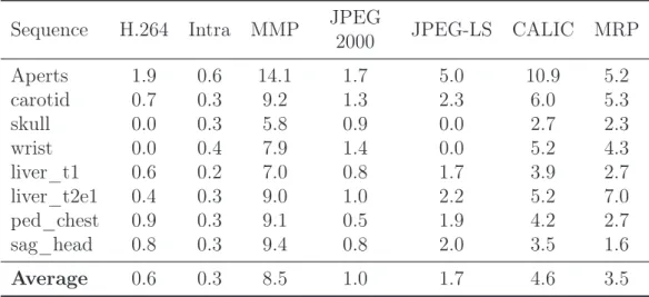
The MMP algorithm performs a flexible block segmentation in the image to encode, with non-overlapping blocks, usually of 16 × 16 pixels. Each block can be further divided using a flexible segmentation, and are encoded in a raster scan order, as can be seen in Figure 2.12. In each block, MMP applies intra prediction, based on the H.264 modes [20]. MMP, however, does not use the traditional transform-quantize-encode paradigm, using instead a dictionary search for its residue encoding. A block-matching is performed be-tween the residue blocks and the dictionary elements. This encoder can also use scale transformations, allowing to match different size blocks. The dictionary is updated with recent encoded residue blocks, to optimise the encoding efficiency.

im-2.3. Lossless coding algorithms 17

Figure 2.12: Flexible block segmentation and partition tree [14]: (a) segmentation of an image block, (b) corresponding binary segmentation tree.

plicit intra prediction mode was added, based on the Least Squares Prediction (LSP) algorithm [43]. Also, the horizontal and vertical modes of H.264 were improved, based on [44], by expanding the neighbourhood to use extra pixels, instead of just the ones on the block edge. Finally, a Differential Pulse Code Modulation (DPCM) technique is also applied for the encoding of the residue for all the prediction modes.

2.3.5

3D-MMP

In [15,17], the MMP encoder was extended into a volumetric compression algorithm, called 3D-MMP. In this implementation the sequence information is treated as a volumetric signal, instead of the usual slice-by-slice approach. The flexible partition used in MMP was extended for 3D blocks, as can be seen in Figure 2.13. Thus, each block can be segmented into three directions: temporal, horizontal and vertically.

3D-MMP also uses a dictionary based approach but 3D blocks pose new challenges, driving to a new dictionary design that uses multiple scaled versions of the dictionary. Therefore, when performing a search, the algorithm only needs to perform it in the corresponding scaled dictionary. This method requires more memory, but the computational complexity is lower than having a single dictionary.

As explained before, MMP uses the intra prediction modes of H.264. In 3D-MMP these modes are expanded to a 3D block basis. Thus, as the neighbour pixels are on the edge of the blocks, the neighbourhood will also be three-dimensional, as can be seen in Figure 2.14. Additionally, the LSP algorithm, based on [45], was also adopted in 3D-MMP and expanded to have a 3D support.

For the compression of video sequences, 3D-MMP, can rearrange the slices by grouping them on the temporal axes, separating the odd and even slices, in a similar way of I-type

Figure 2.13: Triadic flexible partition [17].

Figure 2.14: Block neighbourhood [17].

and B-type slices, as in H.264, as shown in Figure 2.15. This feature adds support for bidi-rectional prediction in 3D-MMP. For instance, the LSP is now able to use reference pixels in future slices. The encoding process may also be sequential without the rearrangement of slices.

This encoder also has a support for lossless compression, using the λ parameter that defines the weight given to the rate-distortion optimisation, that must be set to zero.

2.3.6

H.264 / Advanced Video Coding

The H.264 encoder is a video compression standard [18–20], from ITU and ISO. This is a hybrid encoder, whose algorithm has four main stages: prediction, both intra and inter

2.3. Lossless coding algorithms 19

Figure 2.15: Hierarchical video compression architecture [17].

slice3

, transform, quantization and entropy coding. The structure of the H.264 encoder can be seen in Figure 2.16.

Figure 2.16: Basic coding structure of H.264 [19].

For the prediction the image is divided into macro-blocks of 16×16 pixels. There are three types of slice categories in H.264: I slices, whose macro-blocks are predicted only with intra prediction modes, P slices, additionally to the intra prediction modes the macro-blocks of these slices can also use inter prediction with one motion-compensated reference, and B slices, that additionally to the P slices prediction can use two inter-prediction references. For intra prediction H.264 can divide the macro-blocks into blocks of 4 × 4 pixels. Thus, H.264 allows four intra prediction modes, namely Vertical, Horizontal, DC and Plane. The 4 × 4 block may be encoded with nine prediction modes, as can be seen in Figure 2.17.

3

In this context, the mention to ’slice’ is interchangeable to the use of ’frame’. As the subject of this work is medical imaging compression only the slice expression is used.

Figure 2.17: H.264 intra prediction modes for 4 × 4 blocks [46].

In the inter-slice prediction of H.264, the intra prediction modes can also be used. How-ever, in P and B-type slices motion compensation can also be used, with past or past and future references, respectively. Macro-blocks in the motion compensation can be divided into blocks down to 4 × 4 pixels. For the prediction a precision of up to quarter-pixel can be used.

After the prediction, the Hadamard or Discrete Cosine Transform (DCT) transform is applied to the resulting residual. The transform coefficients are quantised and entropy coded. However, when quantisation is applied the coding process becomes lossy, meaning that part of the information is permanently lost.

Additionally, H.264 allows for lossless compression. In this mode, the transform and quantisation processes are bypassed. The lossless mode of H.264 reference software can only use intra encoding, which is the one used in this work.

2.3.7

High Efficiency Video Coding

The High Efficiency Video Coding (HEVC), also known as H.265, is the most recent state-of-the-art video codec standard [21, 22]. This standard was proposed in order to replace H.264, having as a main goal to improve the compression performance relative to H.264, in the order of 50% bit-rate savings for the same quality.

The H.265 standard shares many of the characteristics of H.264, the main characteristic being the hybrid coding structure. In Figure 2.18, the basic encoder structure of HEVC

2.3. Lossless coding algorithms 21

can be seen.

Figure 2.18: Basic coding structure of HEVC [22].

One of the differences between HEVC and H.264 is the replacement of the macro-block by the Coding Tree Unit (CTU), which can have up to 64 × 64 pixels. The CTU can then be partitioned into smaller blocks using a quadtree-like signalling. The usage of higher size blocks allows for a higher compression efficiency, specially in higher resolution images, and for the use of more prediction modes in the intra prediction. Therefore, HEVC uses 35 intra prediction modes, that can be seen in Figure 2.19. The right side of this figure shows an example of a directional prediction mode of the encoder.

Figure 2.19: HEVC intra prediction modes [22].

As in H.264, H.265 standard relies on motion compensation for the P and B type slices. A quarter-pixel precision is, once again, used to perform the motion estimation.

The HEVC reference software in the lossless mode allows the use of inter prediction, unlike H.264, in such profiles as Random Access or Low Delay. In this mode, the transform and quantisation steps are bypassed, with the residue being encoded with an entropy coder.

Range extension

Like H.264, HEVC has several extensions to its algorithm. For the lossless coding, the Range Extension is of especial interest, HEVC Range Extension (HEVC RExt) [23]. This extension introduced the support for higher bit depth images and different chroma sub-samplings, such as 4:2:2 and 4:4:4. The objective is to perform lossless and screen content compression.

The main focus of this research is the lossless coding of medical images, then, the new HEVC RExt tools for lossless compression are of interest. Some of the changes that ben-efit the lossless coding are: Intra-picture block copying prediction, similar to the motion compensation but for already coded blocks of the same sequence, Smoothing disabling of intra-picture prediction, disables a smoothing filter used in intra pre-diction, Transform skip mode modifications, allows the use of a DPCM vertical and horizontal modes for the the residual signals, when the transform is bypassed. Consid-ering this, we will compare HEVC with its Range Extension for the lossless compression modes.

2.3.8

Minimum rate predictors

The Minimum Rate Predictors (MRP) codec was first proposed in 2000 [24, 25], but has been improved in [26–28]. MRP uses multiple linear predictors adapted to each image, on a Variable Block Size (VBS) basis.

Initially, the image is divided into blocks of 8×8 pixels. These blocks are then sorted in to one of M classes, each class being represented by a different linear predictor, according to the block variance. This information is used as a training set for the design of the linear predictors. All pixels of the same class are then used in Yule-Walker equations. These equations, when solved, return the optimum prediction coefficients, which are then used to calculate the prediction.

For a given pixel, p0, the prediction value given by the m-th class, m = 1, ..., M, is

given by Equation 2.3. The linear predictors are used in order to better estimate the image structures. Each predictor uses K reference pixels, distributed, as can be seen in

2.3. Lossless coding algorithms 23 Figure 2.20, for K = 30. ˆ s(p0) = K X k=1 am(k) · s(pk), (2.3)

In this equation, am(k) is the prediction coefficient for a given pixel, of the m-th class,

and s(pk) is the value of the pk reference pixel.

Figure 2.20: Disposition of reference pixels [28].

After the coefficients and prediction determination, the cost of the prediction error can be calculated, taken as model the generalised Gaussian functions. The context selection for the modelling is given by Equation 2.4:

U = 12 X k=1 1 δk · |s(pk) − ˆs(pk)| , (2.4)

where δk is a weighting factor, indicating the Euclidean distance between p0 and reference

pixel pk, given by Equation 2.5 and s(p0) − ˆs(p0) is the prediction error.

δk =

64

pdx(k)2+ dy(k)2

(2.5)

In Equation 2.5, 64 represents the precision of the weighting factor, 6 bits, dx(k) and

dy(k) represent the distance from the current pixel to the k reference pixel in the X and

Y axis, respectively. Finally, pdx(k)2+ dy(k)2 is the euclidean distance between the k

reference pixel and the pixel for which we wish to determine the context.

The U parameter is closely related to the variance of the prediction error. Thus, the parameter U is an estimation of the variance and it is quantised and calculated for each block. The thresholds for the quantisation are optimised in order to achieve the highest coding efficiency for each class. The blocks are then re-classified, regarding the U param-eter and the context quantisation thresholds. With this new classification, the prediction

coefficients will be determined again, and the process is repeated.

These optimisations are performed in order to minimise the cost function for the encoding image, the cost function is given by Equation 2.6:

J =X

p0

L(e|ˆs(p0), n) + B_a+ B_m+ B_t, (2.6)

where L(e|ˆs(p0), n) is the total code length of the prediction errors and B_a, B_m and B_t

are the code lengths of the prediction coefficients, class selection and context modelling threshold values, respectively.

When this process is concluded, the MRP algorithm has another optimisation loop, using VBS. The block size can now change from blocks of 32 × 32 to 2 × 2 pixels, in a quadtree segmentation structure, that is optimised in order to minimise the cost function. The size of the used blocks highly depends on the local characteristics of the image.

The classes are recursively chosen for each block, regarding to the cost function J. The thresholds, the block classification and the optimum value of the shape parameter, for the probability distribution, are then optimised in a loop. If the optimisation flag is activated, two prediction coefficients are randomly chosen and a partial optimisation is performed by slightly varying their values. These optimisations are repeated several times for each class. The arithmetic encoding of all the needed parameters is performed by a range coder [47], or by a simple Huffman coder.

One of the main characteristics of MRP is the fact that it minimises a cost function, representing the amount of prediction error data, instead of minimising a sum of least-squares of the prediction errors, as done by other encoders. The prediction order, K, and the number of classes, M, can be determined from the dimensions of the encoding image. Thus, selecting appropriate values for these parameters .

2.4

Lossess codec comparison

In this section, the previously described lossless encoders will be compared, when applied to the compression of medical images. To evaluate these encoders, the test images were encoded with the parameters set to lossless compression. Publicly available software implementations of these encoders were used for the tests.

The CALIC and JPEG-LS encoders were used with their default configuration values for lossless compression. For the MRP algorithm, the extra optimisation flag was activated,

2.4. Lossess codec comparison 25

with the remaining options set by the encoder.

In the MMP encoder, the fast implementation was used, and the default dictionary size was used. In 3D-MMP the λ parameter was also set to zero, the block size was of 16×16×4 pixels, in the Y ×X ×Z format, and the prediction level was set to 8, indicating the minimum partitioning size to use prediction. In 3D-MMP the hierarchical video compression was used, and the dictionary was set to use a maximum of 5000 elements. For JPEG2000, the software implementation OpenJPEG v2.1 is used with the default con-figuration. This software also includes an implementation of JP3D, which was configured to use a 3D-DWT and 3D-EBCOT.

For H.264/AVC, the latest release of the reference software JM 18.6 was used. For lossless coding, FRExt High 4:4:4 Profile was used for Intra coding, with QP and QP Offsets set to 0.

As for HEVC, the reference software HM 16.4 was used, both for Intra Main and Random Access profiles. In the lossless coding mode, QP was set to 0, and both Transquant-BypassEnableFlag and CUTransquantBypassFlagForce were set to 1. For the remaining configuration parameters the default values were used. HEVC RExt is included in the same reference software as HEVC. The same parameters, as in HEVC, were used with the same values. The HEVC RExt specific parameter CostMode was set to lossless. For the lossless coding modes, only the JP3D, 3D-MMP, H.264 and HEVC encoders can have a sequence as the input. All other encoders only use intra prediction, for these each slice in a sequence is encoded independently and the result is the average of all the encoded frames. Only, JP3D, 3D-MMP and HEVC Random Access (HEVC RA) can exploit the inter-slice redundancy.

Lossless compression was chosen for this work, as it is often a requirement for the compres-sion of medical images, as stated in Section 2.2. For instance, when reversibly compressed images are used for the diagnosis, possible compression artefacts are not an issue. The results for these encoders, in bits-per-pixel (bpp), are shown in Table 2.3, for the image encoders, in Table 2.4, for the video/volumetric encoders, and in Table 2.5 for 3D-MMP. The 3D-MMP encoder requires that the number of slices of the input sequence to be multiple of the block size in the Z direction. Therefore, the results of this encoder are not directly comparable with the remaining encoders. In Table 2.5 the number of slices used in 3D-MMP are also shown. In Chapter 3, we show a table of encoding results for these encoders in which the number of slices is multiple of 16, see Table 3.2. Therefore we can compare the sequence Aperts as it uses the same number of slices in both tables, for 3D-MMP. It can be observed that, for that particular sequence, the compression efficiency

Table 2.3: Performance comparison of the image encoders (results in bpp). Sequence H.264 HEVC Intra RExt Intra MMP JPEG 2000 JPEG-LS CALIC MRP Aperts 1.193 1.289 1.136 1.178 1.261 1.058 0.998 0.775 carotid 2.062 2.198 2.001 1.977 2.019 1.778 1.684 1.374 skull 3.183 3.083 2.890 2.959 2.991 2.761 2.628 2.329 wrist 1.911 2.195 1.890 1.717 1.757 1.627 1.550 1.173 liver_t1 3.489 3.742 3.400 3.393 3.256 3.160 3.022 2.582 liver_t2e1 2.806 2.811 2.561 2.460 2.572 2.418 2.269 1.722 ped_chest 3.080 3.352 3.051 3.074 3.021 2.937 2.789 2.337 sag_head 2.635 2.732 2.594 2.808 2.905 2.582 2.519 2.279 Average 2.545 2.675 2.440 2.446 2.473 2.290 2.183 1.821

Table 2.4: Performance comparison of the video encoders (results in bpp). Sequence HEVC R.A. RExt R.A. JP3D

Aperts 0.826 0.728 0.941 carotid 1.587 1.425 1.547 skull 1.905 1.766 2.088 wrist 1.155 1.002 1.238 liver_t1 2.392 2.052 2.356 liver_t2e1 1.726 1.510 1.745 ped_chest 1.699 1.534 2.071 sag_head 1.873 1.748 2.160 Average 1.645 1.471 1.768

of 3D-MMP is similar to that of JP3D. Finally, the tests were not performed to all the sequences due to the computational complexity of the encoder. For the Aperts sequence, for instance, the encoding process took 4128742 seconds, which is equivalent to almost 48 days. Hence, and also due to its compression efficiency, 3D-MMP will not be used in the remainder of this work.

The remaining two tables show the results for the image and video encoders. In these tables R.A. means the Random Access profile, and RExt means the HEVC RExt encoder. As expected, it is possible to see that encoders which are able to exploit the inter-slice redundancies in a sequence, generally present better results. The best overall results, on average, are obtained for HEVC RExt with the Random Access profile. This was expected as HEVC is the state-of-the-art video encoder, and its Range Extension has several tools that improve the lossless compression of sequences. It can also be observed from Tables 2.3 and 2.4 that the Range Extension of HEVC improved the lossless compression efficiency of this encoder, with an improvement of roughly 0.2 bpp.

2.5. Other state-of-the-art techniques 27

Table 2.5: Compression results of the 3D-MMP (results in bpp). Sequence Slices 3D-MMP Aperts 96 0.938 carotid 72 1.622 skull wrist liver_t1 56 2.579 liver_t2e1 56 2.051 ped_chest 76 1.804 sag_head 56 2.303

explained by the encoder prediction efficiency, as the linear predictors are suitable to describe several image structures and they are optimised for the input image. MRP has results that are close to that of the video encoders, at the level of JP3D, with a difference of 0.05 bpp, and without inter-slice prediction support. For the HEVC encoders this deviation is higher, with 0.18 bpp for HEVC RA and 0.35 bpp for HEVC RExt R.A. The encoding efficiency shown by MRP was one of the reasons that this encoder was chosen as main object of our research.

2.5

Other state-of-the-art techniques

In this section a general overview of state-of-the-art research is presented. Current research orientations are discussed, for instance, scalable compression, lossy-to-lossless compres-sion, Region of Interest (ROI) comprescompres-sion, etc.

2.5.1

Scalable lossless compression based on global and local

sym-metries for 3D medical images

Medical images usually contain inherent symmetries that can be exploited for their com-pression. Victor Sanchez, et al, in [48, 49], propose to exploit these symmetries as a prediction method. The paper shows that medical images have both global and local symmetries, as seen in Figure 2.21.

The first step in the proposed procedure is to decompose the image in n frequency sub-bands using a 2D-DWT, as the symmetries remain after the transform. Then a block-based prediction is applied, followed by the entropy coding of residual data and transfor-mation parameters. In the block-based intra-band prediction each sub-band is divided in blocks of 16 × 16 coefficients. Eight spatial transformations are used for the prediction.

(a) Global symmetry.

(b) Local symmetry.

Figure 2.21: Example of the possible symmetries in medical images [48].

These transformations (see Table 2.6) are applied to each already encoded block in the image. The block and transformation pair that best approximate the current block are selected. The blocks of 16 × 16 coefficients can be further divided into sub-blocks of 8 × 8 and 4×4 coefficients, if this operation results in a compression performance improvement. For the compression of the prediction information the authors use variable length codes. For the residue encoding a modified EBCOT is proposed. The paper shows that this method achieves an average improvement of 15% in compression ratio over JPEG2000 and H.264, for lossless compression [48]. Also, this method allows for scalable lossless compression of 3D medical image data.

In [49] some improvements are made to the previous method. Additionally to the previous spatial transformations prediction, the authors added inter-slice prediction and global

2.5. Other state-of-the-art techniques 29

Table 2.6: Spatial transformations [48].

symmetry detection. Figure 2.22 shows the block diagram of this method.

The global symmetry is detected using a Fourier-Melin transform. This symmetry is used to assess the scanning order of the blocks. The image is divided in two areas, A and B, regarding the global symmetry. After a block in area A is processed, the next block is the symmetrical positioned block in area B. This allows the prediction to exploit the global symmetry. The spatial transformations prediction of Table 2.6 are then applied to each block.

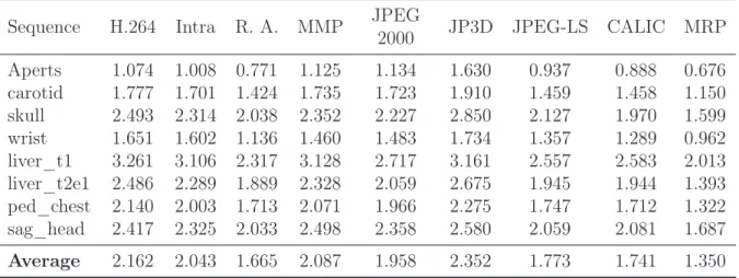
For the inter-slice prediction a DPCM mode is used. This mode is used to exploit the correlation between sub-band coefficients in adjacent slices. The DPCM mode can be used

Figure 2.22: Block diagram of the symmetry based scalable lossless compression tech-nique [49].

in five directions, as seen in Figure 2.23. The entropy coding is once again performed using EBCOT. The results show compression efficiency gains of 1%, when compared with the previous method.

Figure 2.23: Five proposed prediction modes for inter-slice DPCM prediction [49].

2.5.2

Hierarchical oriented prediction for scalable compression of

medical images

Jonathan Taquet, et al, propose in [2, 50] a Hierarchical Oriented Prediction (HOP) method for the scalable compression of medical images.

Each prediction level of the HOP algorithm is performed in two steps, as seen in Fig-ure 2.24. In the HStep a horizontal prediction of odd indexed pixels is performed, using already known, causal, pixels. With this step, the image is horizontally sub-sampled. The VStep, performs the same operation but in the vertical direction of the sub-sampled image.

2.5. Other state-of-the-art techniques 31

Figure 2.24: One prediction level of the HOP algorithm [2].

The HOP algorithm is designed for prediction of sharp edges in noisy images. An orien-tation estimation inspired by GAP is performed. This estimation allows the algorithm to choose between five predictors, to perform the prediction along edges. A predictor for homogeneous areas is also available. Additionally, a least-squares estimation can also be performed. This estimation uses an extended set of the causal pixels to perform a dynamic prediction. Therefore, it results in a better adaptation to the image characteristics. The described predictors are used in the HOP algorithm process, for the prediction of odd pixels. In order to avoid systematic errors resulting from static predictors, a prediction bias cancellation is used.

For the coding stage, a residual remapping technique is used before the entropy coder. The authors also extended the proposed algorithm for near-lossless compression. Finally, the results show that, on average, this algorithm is 6.5% more efficient than JPEG2000 and 2.1% than CALIC.

2.5.3

Compression of X-ray angiography based on automatic

seg-mentation

Zhongwei Xu, et al, propose in [51] a diagnostically lossless compression method for X-ray angiography images. This method is based on automatic segmentation of the images, using ray-casting and α-shapes.

Medical images in general, and angiography images in particular, often have a ROI and a background region. The proposed method exploits this fact, essentially by removing the background region before feeding the resulting image to a lossless encoder. As only the background region is removed, this method is diagnostically lossless.

X-ray angiography images are essentially radially symmetric, the method exploits this characteristic to differentiate the ROI from the background region. Initially a pre-processing step is executed in which slice averaging and noise reduction are performed to