An exact solution for tube and slit flow of a FENE-P fluid

Acta Mechanica 158, 157 167 (2002)

ACTA MECHANICA

9 Springer-Verlag 2002

An e x a c t s o l u t i o n f o r t u b e and slit flow

o f a F E N E - P fluid

P. J. Oliveira, Covilhg,, Portugal

(Received September 20, 2001; revised March 11, 2002)

Summary. A fully analytical solution is derived for rectilinear flow of a nonlinear viscoelastic fluid obey- ing the constitutive FENE-P model, under fully developed conditions. Both the plane case (slit flow) and the axisymmetric case (tube flow) are considered. Physical interpretation of the results is provided. The normal stress profile is found to vary in a non-monotone way with the dimensionless parameter character- izing viscoelasticity, the Deborah number

(De).

For Deborah numbers below a critical value (dependent on the extensibility parameter of the model L 2) the normal stress raises with elasticity, but this trend is reversed for values above the critical one. This effect is due to the competing influence of elasticity and shear thinning. Also, as a consequence of shear thinning the velocity profile becomes flatter as De increases and L 2 decreases, leading to higher flow rates for the same pressure drop.

1 Introduction

Interest in analytical studies of flow problems involving viscoelastic fluids has been growing, as a cursory overview o f the contents of a specialized journal reveals; for example, H a y a t et al. have tackled some time-dependent problems with the second-order Rivlin fluid [1], [2], and also with the Oldroyd-B fluid [3]. While these are useful theoretical works, it should be pointed out that the second-order fluid is hardly ever used to represent real fluids as it pos- sesses a negative first-normal stress coefficient, contrary to what is observed, and the Old- royd-B is a quasi-linear model having a constant viscosity. Models used to represent actual polymeric fluids are usually more complex than the above, being nonlinear in the stresses and with implicit differential constitutive equations relating stress with strain rates. Typical models o f this kind, often used in simulation works, are the Phan-Thien - Tanner model [4], the F E N E - P model [5] and the Giesekus model [6].

tn this note we derive analytically the solution for the problem of fully developed flow of a F E N E - P fluid flowing either along a circular cross-section tube or within the space between two parallel plates (slit flow). Due to the intrinsic nonlinearity o f the F E N E - P constitutive model, it has apparently gone un-noticed that such solutions can be easily worked out for the particular situation considered here, o f fully-developed flow conditions, as will be shown. Analytical solutions for simple flows o f viscoelastic fluids are useful per se, as they allow a complete description o f the flow with given explicit expressions (in some cases the solution is only implicit), and are also useful to be applied as b o u n d a r y conditions in computational simulations, with the benefit o f allowing a reduction of the size o f the computational domain.

W i t h o u t the worry of being exhaustive, we give below a brief overview o f some related analytical works. In the early days of rheology, Rivlin [7] gave the solution for Poiseuille

158 P.J. Oliveira flows of the Reiner-Rivlin fluid and, a few years later, Oldroyd [8] indicated how the solution for rectilinear flows of his general 8-constant fluid model could be constructed by following a general "indirect" procedure in which the shear rate was taken as the independent variable instead of the lateral position (in this case we cannot say that the solution is fully analytical). That procedure was adopted by Walters [9] who derived solutions for a general linear equa- tion of state in a number of flow configurations, and much later Schaftingen and Crochet [10] followed the same steps to give an implicit semi-analytical solution for pipe flow of the John- son - Segalman fluid. For the Giesekus model, in the absence of solvent stress contribution, analytical solutions for channel and pipe flows were first given by Yoo and Choi [11]. The final expressions were not totally explicit, as a non-linear equation had to be solved for the pressure-gradient, and so some form of iteration was still required. Later, Schleiniger and Weinacht [12] derived identical expressions for the "classical solution" of Poiseuille flow of the Giesekus fluid, but have also analyzed "weak solutions" and gave semi-analytical expres- sions for the case with solvent contribution, in which an implicit procedure along the lines of that of Oldroyd and Walters is required. For the Phan-Thien/Tanner model (with parameter = 0), we have derived analytical expressions for both the linear and exponential forms of the model [13] and have also considered the related thermal problem including viscous dissi- pation [14]. Generally, it is easier to obtain a solution when the axial pressure gradient is known. However, we are more interested in the situation in which the average velocity (or flow rate) is known and the pressure-gradient unknown, as this corresponds to the situation most often found in practice. It is this situation, for the FENE-P fluid, which is analyzed here.

2 Analysis

The FENE-P model is based on the kinetic theory for finitely extensible dumbbells and, when the Peterlin approximation for the average spring force is introduced, it leads to a differential constitutive equation which was given in the original paper (Bird et al. [5]) in terms of the extra stress tensor x. Following Chilcott and Rallison [15], we prefer to work here with the model expressed in terms of a configuration tensor A defined by A = 3(QQ)/Q~ 2 where Q is the end-to-end vector connecting the dumbbell beads, (.) indicates an ensemble average over the configuration space, and Q~ is an equilibrium length. The connector force of the spring in the original FENE model follows the expression proposed by Warner:

H

F c = Q , (1)

1 - ( q . q)/Q02

where H is the spring constant and Q0 the maximum possible spring length. In order to derive an evolution equation for the configuration tensor, the average (QF ~} is required, and it is not possible to obtain a closed-form equation unless some form of approximation is intro- duced. In the FENE-P model (P for Peterlin), Eq. (1) for the spring force is approximated by:

H

FC "~ 1 - ( Q . Q } / Q o 2 Q - f H Q , (2)

following an idea suggested by Peterlin (see Bird et al. [5]). By using the definition of A given above, we see that the dimensionless function f defined by the last term in Eq. (2) depends on the trace of A and can be written as:

L 2

(3)

Tube and slit flow of a FENE-P fluid 159 where L 2 =_ 3Qo2/Qe 2 is called the extensibility p a r a m e t e r of the model. It represents the square o f the ratio between the m a x i m u m and the equilibrium lengths o f the spring, and it is related to "b" used in the original Ref. [5] by L 2 = b + 3 (Note: b =- HQo2/IcT; I~ is the Boltz- m a n n constant and T the absolute temperature).

At this point it is possible, after ensemble averaging the equations of m o t i o n for the d u m b - bells, to derive the evolution equation for the configuration tensor of the F E N E - P model as

([5], [16]):

v 1

A = - ~ (XA - aI) (4)

which needs to be solved together with K r a m e r s ' form for the relation linking A to the poly- mer stress,

%

= ~- ( / A - a I ) . (5)

In these equations the constant model parameters are the polymer viscosity ~p, the relaxation time A, and the extensibility p a r a m e t e r L 2. The additional p a r a m e t e r a is not an independent parameter; it is a short notation for a - 1/(1 - 3 / L 2) which arises in the derivation. It is related to physical properties by a = 1 + 3kT/HQo 2 and to the original b p a r a m e t e r [5] by

a = (b + 3)lb. Some times a m o r e simplified version of F E N E - P is utilized, in which a = 1 on

the assumption that L 2 is large. However, there is a certain tendency seen in the recent litera- ture to a d o p t low values for L 2 (e.g. [16]), and in this case it is not adequate to consider a = 1, so we leave it in the model equations and take account o f it in the analysis.

The symbol v in Eq. (4) is used to denote Oldroyd's upper convected derivative, v D A

A - D t A - V u - V u T . A , (6)

where u is the velocity vector, the material derivative is D / D t ~ 0 / 0 t + u - V, and V u T is the transpose o f the velocity gradient. By combining Eqs. (4) and (5), we have:

V ,g

A : - - - . (7)

rb

This constitutive equation is to be solved in conjunction with the continuity and m o m e n t u m equations, respectively:

D u

V . u = 0 and ~ O D t = - V p + V . ~ , (8)

where incompressible flow is assumed and p is the pressure. In general, the operator v satis- fies:

v v D f

( f A ) = f ( A ) + A D~

(9)

for any function f. But, for the situation of fully-developed, steady and rectilinear flow, in which the only nonzero velocity c o m p o n e n t is u (v = w = 0), which is aligned with the flow direction x, we have:

o f

D f Of Of + v ~ + w ~ f x = U ~ x x 0

160 P.J. Oliveira and so, from Eq. (9),

V V

( f A ) = f A . (10)

It is this result which allows an analytical solution to be obtained. If we apply the upper convected operator v to Eq. (5), we obtain

v 89 v v % v

= 7 ((fA) - aI) = 7 ( f A + 2 a D ) ,

V

where we used the result I = - 2 D , with the rate-of-strain tensor denoted by D = (Vu + VuT). The latter equation is made explicit on A and equated to (7), to obtain a final expression for the FENE-P model in terms of the extra stress:

~7

At + f~ =

2a~pD.

(11)

The function f should now be expressed in terms of the main dependent variable ~, and this is accomplished by taking the trace of Eq. (5) to get:

), 3a + -- tr

trA

- ~P

f

which is then introduced into the definition of f (Eq, 3) to yield: A

3a + - - trlr

1 + L ~ L (12)

f

For the problem under consideration the constitutive equation (1 l) reduces to the set:

du (13)

f~=xx = 2Ar~y d ~ '

.f%y = 0, (14)

du du (15)

which is valid for both the plane and axisymmetric cases (with the radial coordinate r substi- tuted for the lateral coordinate y). The continuity equation is satisfied identically, and the momentum equation (8) reduces to:

=

p~

( 1 6 )

~-~ P y and T~ = 2

for the plane and axisymmetric cases, respectively, with P - d p / d x denoting the applied (but unknown) pressure gradient. After dividing Eq. (13) by Eq. (15), so that the function f cancels out, we obtain for the normal stress:

2A p2y~ 2A p~ r 2

7-xx- m ~ d Txx-- - - (17)

Tube and slit flow ofa FENE-P fluid 161 Once rxx = tr~ is known, the function f can be determined from (12), and Eq. (15) gives directly the velocity gradient, which is conveniently expressed in nondimensional form as

ds 3X d~) a d s 4x?vI_~ d+ a

[

3a + 18De2X2~12/a] 9 1 q -~- ] (slit), 3a + 32De2X2+2/a]

-] (tube),

(18)

after scaling y (or r) with the half-slit width H (or the tube radius R) and u with the average velocity U. So in Eqs. (18), and in what follows, we have introduced the notation g ~ u/U,

9 - y/H, + - r/R, and the Deborah number, used to characterize viscoelastic effects, is

defined as usually, De = I U / H or De = AU/R. The nondimensional pressure gradient para- meter X is defined as

X =UN _{with Ux - - P H 2 (slit) or U N -} _ p R ~ _{(tube), (19)}

U ' 3r/; 8%

and it is clear that Ux has the meaning of the average velocity for the Newtonian case. Inte- gration of Eqs. (18) from a general lateral position (? or ~)) to the wall (+ = 9 = i), where a no-slip boundary condition is imposed, gives the velocity profiles:

{(~): x(i-9

2) 1 + 9 ~

[

z)~x2 (1

+ +~)]

(tube)

9

~2(+)

:2X(1-+2) i+16

(2o)

It is interesting to note that the first two terms in the brackets of Eq. (18), (1 + 3a/L2)/a,

become equal to unity due to the definition of a, with the consequence that the velocity pro- files (20) reduce to the parabolic Newtonian profile whenever De tends to zero (irrespective of L2), as it should. Otherwise, the solution at De = 0 would still depend on the viscoelastic- related parameter

L 2,

in what would be an incorrect conclusion. A further integration of the velocity profiles across the slit or tube sections, together with the definitions of the average velocity in the cross section, which in nondimensionaI terms are:

1 1

1 = f~2(9) d9 (slit) and I = f2~%(+) +d+ (tube)

0 0

gives the following cubic equation for X:

1 = x ( 1 + 9 x 2)

with

;~_

54 D~ 2 (slit) oi- 9 - 64 D ~ 2 ( t u b e ) . (21)

5 a2L 2 3 a2L 2

The real solution of this cubic equation is:

X - 432U6(D2/3 - 22/3)

162 P.J. Oliveira with:

D = (4 + 27/3) 1/2 + 33/2/32/2 ,

and where the appropriate/3, f r o m Eq. (21), should be used for the slit or the tube flow. At this stage the pressure-gradient p a r a m e t e r X is k n o w n Eq. (22), the velocity profile is given by Eqs. (20), and the stress c o m p o n e n t s can be obtained f r o m Eqs. (16) and (17). After being scaled with the wall shear stress for the Newtonian case, the stress c o m p o n e n t s are writ- ten in nondimensional form as:

Txv - 7"w

= -X{I

(slit),

(23)

Tx, -- ~-x,./ (4rlp U)

= - X e ( t u b e )

for the shear stress components, and

(24)

Tx= - ~'xx

= 8DeX2§

(tube)

for the n o r m a l stress components. It is noted that the wall shear stress for the upper-convected Maxwell model, for example, is identical to that for the Newtonian fluid. In this sense, it is better to view the normalized stresses in Eqs. (23) and (24) as being scaled by a factor p r o p o r - tional to a constant viscosity % multiplied by a constant typical shear rate,

U/H

or

U/R.

3 Discussion and conclusions

The physical interpretation o f the results is facilitated by a few graphs showing the variation of velocity and stresses. Representative velocity profiles for the tube flow are shown in Fig. 1 for fixed extensibility p a r a m e t e r L 2 = 10 and increasing D e b o r a h number, and in Fig. 2 for fixed

De

= 2 and increasing L 2. The range of L 2 (10, 100 and 1 000) is that usually found in works with the F E N E - P or F E N E - C R (constant viscosity, [15]) models (e.g., [15], [16]). It is seen that b o t h an increase o f the D e b o r a h n u m b e r or a decrease o f the extensibility p a r a m e t e r lead to flatter velocity profiles as a consequence of enhanced shear thinning in viscosity.

W h e n L 2 tends to infinity the function f tends to unity (cf. Eq. (3)), and the constitutive equations (4) and (5) reduce to the well-known upper-convected Maxwell ( U C M ) model, writ~

v

ten in terms o f 9 as ) ~ + 9 =

2rlpD

(this is m o r e directly seen f r o m Eq. (11) with f ~ 1 and a --+ 1, as L 2 ---+ oc). The U C M model is a particular f o r m o f the Oldroyd-B family with a van- ishing solvent viscosity; it represents a fluid molecule with infinite extensibility and has a very simple solution in fully developed flow: the velocity profile is parabolic as for the Newtonian fluid, and the n o r m a l stress is quadratic in the velocity gradient, ~-x~ =

2Arlp(du/dy) 2.

This trend o f L 2 on the velocity variation is clearly seen in Fig. 2 when L 2 ---+ oo, with the shape o f the profile approaching that for the N e w t o n i a n fluid; the velocity solution Eq. (20) gives this limit readily: L 2 ~ oo ~ X --+ 1 Eq. (21), so the term in the square brackets o f Eq. (20) goes to unity, and the parabolic profile is recovered.

Tube and slit flow of a FENE-P fluid 163 2 . 0 I I I I I I I I I I 0 "X~ g 0 5 . . . . O e = l "~,\ 4 - - - De--2 ~\ 1 . - - o ~ = s ", | ~ L i I q I i I i ] O. 0 0 . 2 0 . 4 O. 6 0 . 8 1

~/R

Fig. 1. Velocity profiles in tube flow for varying Deborah number (fixed L2= 10) 1. 0 %Z-,. \.. o ~ q . . . L ; = ~ ~ j I - - L ' = i O 0 '~.' |

!

- - L L ~

" % /

0 I k I * 1 [ I o o 0 2 0 4 0 6 0 8 r / R

Fig. 2. Velocity profiles in tube flow for varying extensibility parameter of the FENE-P model, I9 (fixed De = 2)

1 0 ~ l i l / l l I q i i LIB I I i ILIIL I I I i j r _ __ L 2 2 = 1 0 ~ ' - . ~ ~0 7 - - - L = 1 0 0 0 . - " ~ ~ . . ~ 10 ~ - / - " g ' 7 Z / / ' 1 0

1

~ o - '

I ~

7

1

~ '.L;'~'I

I '1'Jl'[

10 -~ 1 10 10 2 10 ~ 7?,

Fig. 3. Shear viscosity and first nor- maZ stress difference for the FENE-P fluid in simple shear flow

At this point it is worth emphasizing that Mthough the viscosity parameter o f the model %

is a constant, the viscosity function as defined by r}(~) -

rxy/~

in a simple shear flow (of shear

~) is not, and tends to decrease with ~/. This is illustrated in Fig. 3 where the material proper- ties (viscosity r/(-)) and first normal stress difference NI(~), e.g. [16]) of the F E N E - P fluid in simple shear flow are given as a function of the dimensionless shear rate (equal to ha/, and so

164 3 - 2 -- b-- 1 - - 0 -- 0 . 0 _ J 0 . 2 - - D e = O . 5 O e : l _{/ ,.} - - - D e = 2 - - D e = 5 , / , ' / - - - - O e = l O

,'~"//,,

,;.S / / / J / . y " / / . J ~ ' Y 0 . 4 0 . 6 0 . 8 1 . 0 r/R P. J. Oliveira

<

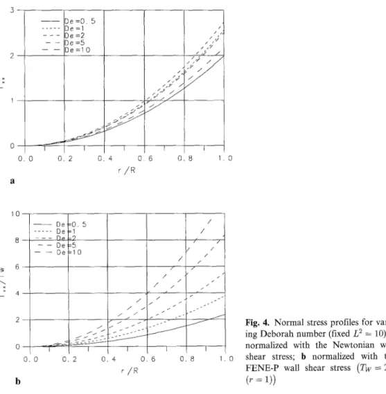
1 0 - - 8 - - 6 - - 4 - 2 - 0 m 0 . 0 - - D e D e D o - - D e - - - - D e = 0 . 5 =1 - ? =5 : 1 0 J 0 . 2 0 / / / / / / / / / / / / / . / / 4 0 . 6 0 . 8 1 . 0

Fig. 4. Normal stress profiles for vary- ing Deborah number (fixed L 2 = 10); a normalized with the Newtonian wall shear stress; b normalized with the FENE-P wall shear stress (Tw = Tx~

(~ : i))

it can be viewed as a Deborah, or more appropriately Weissenberg number). There is shear thinning in both viscosity and first normal stress coefficient k~l = N1/~2; for large ~/, viscosity decreases as r/(+) ~ ~-2/3 and normal stress increases as N1 ~ ~9/a, a w e l l - k n o w n result [16]. For the tube and slit flows under consideration, things are not so simple because the shear rate ~/, equal to d'u/dr or du/dy, is itself an u n k n o w n o f the problem (given by Eqs. (18)) which varies over the cross section and depends in a complex way on both D e and L <

The stress c o m p o n e n t s (Tx~. and Txx) also s h o w the expected effect o f shear thinning, but the normal stress Txx exhibits a n o n - m o n o t o n e behaviour with D e (Fig. 4 a): Tx~ first increases with D e (at fixed L 2 = 10), but at higher De it shows the opposite trend. This is because T~x is affected by elasticity (directly proportional to De) and also by shear thinning (inversely pro- portional to the 4/3 power o f De), c.f. Eqs. (24) and (21) at high De. For this reason, it is bet- ter to plot the normal stress scaled with the wall shear stress o f the F E N E - P fluid, as s h o w n in Fig. 4 b where profiles o f ~-x~/(T~)w m are given, thus removing the shear-thinning effect. A similar conclusion was found for the Phan-Thien/Tanner model [13], and for the Giesekus model as well [17], and therefore it is reasonable to admit that it represents a general feature o f constitutive models exhibiting shear thinning.

For the situation depicted in Fig. 4, with L 2 = 10, the critical De corresponding to the m a x i m u m level o f T ~ is around 2; for higher L s, the critical D e is increased. This is illustrated

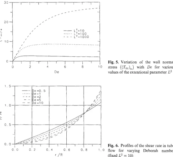
Tube and slit flow of a FENE-P fluid 165 5 O 2 O F- v 1 0 I I I I I I I I L / / / / / / L 2 = I 0 _ / . . . . L 2 = i 0 0 / - - - L 2 = I 0 0 0 / / / - / , P 1 i I i I i I 2 4 6 8 1 0 D e

Fig. 5. Variation of the wall normal

stress ((T,.~.)~,) with De for various

values of the extentional parameter [2

1 . 5 - - - - D e = 0 . 5 D e = l - D e = 2 - - D e = 5 - - - - D e = l O t . 0 - I 0 . 5 -

o, o - ' ~ ' - ~ J ~

~1

0 0 0 . 2 0 . 4

t

//z/."

/

z'f'" I 0 . 6 0 . 8 0 r / R

Fig. 6. Profiles of the shear rate in tube flow for varying Deborah number (fixed L 2 = 10)

in Fig. 5 which shows the normal stress at the wall ((%~),, = r:~(~ = 1)), normalized with the

fixed scale 4wpU/R, as a function of the overall Deborah number De. It is possible to find the

critical Deborah number Dec giving a local maximum o f the wall normal stress for any given

L 2 by calculating the derivative of rxx with respect to De (from Eq. (24)) and equating it to

zero. The final result is not amenable to an analytical expression but we have found, based on a numerical solution, that it can be conveniently expressed by the correlation:

D e c = 0 . 5 0 7 ( L 2 ) 0476 . ( 2 5 )

This correlation enables the calculation o f the critical Deborah number to within 2% for L 2

above 10, say from 30 up to 1 000. For lower values of L2(L 2 <_ 10), Dee actually increases

with decreasing L 2, due to the effect o f the parameter a in the solution, but this range o f L 2 is o f little practical interest.

There is no contradiction between the above finding on the maximum o f the rx~ variation and the fact that the first normal stress difference is a m o n o t o n i c increasing function of A+, as seen in Fig. 3. Recall that D e is a global nondimensional group characterizing the viscoelasti- city o f the flow, and should not be confused with a possible local Deborah number defined as

De' _ A~, with x / = du/dr. To show how complex the situation would be, we present in Fig. 6

profiles o f normalized shear rate (from Eq. (18) for tube flow, divided by the factor 4) at

L 2 = 10 and for increasing values of De. It can be seen that there is a change o f the trend on

166 P.J. Oliveira 2 l . 0- 0 . 8 - - 0 . 6 - - 0 . 4 - - 0 , 2 - - 0 . 0 0 . 0 \ - - De = 0 . 5 "~ ~. ~ . . . De =1 ~. - - - D e = 2 ~ ~ ~ ~ ~ - - D e = 5 -- -- De =1 0 I t I J I I I I 0 . 2 0 . 4 0 . 6 0 . 8 r / R 1 . 0

Fig. 7. Profiles of the shear viscosity function in tube flow for varying Deborah number (fixed L 2 = 10)

X 1 . 0 " - ] ~ ] I I ] t f I I 0 . 4 " - - _ _ _ . . _ O. 2 - - L 2 = 1 0 . . . . L 2 = 1 0 0 _ L 2 = l O 0 0 0.0 I r i 2 4 6 8 D e 1 0

Fig. 8. Variation of the pressure-gra- dient parameter X = UN/U with the Deborah number, at various L 2 (tube flow)

will certainly provoke the non-monotone behavior of the normal stress seen in Fig. 4 a. The viscosity function ~](+), on the other hand, shows the expected shear thinning behaviour, with the r/(,~) versus r profile decreasing all over the tube cross-section when De is raised (Fig. 7).

In what regards an equivalent to the well-known Hagen-Poiseuille result for the flow rate (Q) versus the pressure-drop (Vp), which is @v = r for Newtonian fluids (viscosity #) in a tube with length ~, we obtain for any constitutive model:

Q _ 1 (26)

Q~

X '

where, for the FENE-P fluid in particular, X is given by Eq. (22). As a consequence, the flow rate increases with the Deborah number and decreases with the extensibility parameter of the FENE-P model (see Fig. 8). At high elasticity, the asymptotic behavior is Q/QN ~ (De~L) 2/3.

In conclusion, an analytical solution for the flow of a FENE-P fluid in ducts of circular or planar cross-section was derived and is given in terms of velocity profiles Eqs. (20), stress pro- files Eqs. (23) and (24) and shear rate Eqs. (18). The most important effect was found to be that due to shear thinning, inducing flatter velocity profiles and lower shear stresses. How- ever, for the normal stress there is a competing influence of elasticity and shear thinning. For values of De below a critical level (given by Eq. (25)), elasticity increases the normal stresses in the cross section; for higher values of De, shear thinning reverses this trend, and the normal stresses tend to decrease with De.

Tube and slit flow of a FENE-P fluid 167

References

[1] Hayat, T., Asghar, S., Siddiqui, A. M.: Periodic unsteady flows of a non-Newtonian Fluid. Acta Mech. 131, 169-175 (1998).

[2] Hayat, T., Asghar, S., Siddiqui, A. M.: On the moment of a plane disk in a non-Newtonian Fluid. Acta Mech. 136, 125-131 (1999).

[3] Hayat, T., Siddiqui, A. M., Asghar, S.: Some simple flows of an Oldroyd-B fluid. Int. J. Engng Sci. 39, 135-147 (2001).

[4] Phan-Thien, N., Tanner, R. I.: A new constitutive equation derived from network theory. J. Non- Newtonian Fluid Mech 2, 353-365 (1977).

[5] Bird, R. B., Dotson, P. J., Johnson, N. L.: Polymer solution rheology based on a finitely extensible bead-spring chain model. J. Non-Newtonian Fluid Mech. 7, 213-235 (1980).

[6] Giesekus, H.: A simple constitutive equation for polymer fluids based on the concept of the deforma- tion dependent tensorial mobility. J. Non-Newtonian Fluid Mech. 11, 69 109 (1982).

[7] Rivlin, R. S.: PoiseuilJe flow in a circular tube. Proc. Camb. Phil. Soc. 45, 88-91 (1949).

[8] Oldroyd, J. G.: Non-Newtonian effects in steady motion of some idealized elastico-viscous liquids. Proc. Royal Soc. A 245, 278 -297 (1958).

[9] Walters, K.: Non-Newtonian effects in some elastico-viscous liquids whose behaviour at small rates of shear is characterized by a general linear equation of state. Q. J. Mech. AppI. Math. 15, I, 63-76 (1962).

[10] Van Schaftingen, J. J., Crochet, M. J.: Analytical and numerical solution of the Poiseuille flow of a Johnson- Segalman fluid. J. Non-Newtonian Fluid Mech. 18, 335-351 (1985).

[11] Yoo, J. Y., Choi, H. C.: On the steady simple shear flows of the one-mode Giesekus fluid. Rheol. Acta 28, 13 - 2 4 (1989).

[12] Schleiniger, G., Weinacht, R. J.: Steady Poiseuille flows for a Giesekus fluid. J. Non-Newtonian Fluid Mech. 40, 79-102 (1991).

[131 Oliveira, P. J., Pinho, F. T.: Analytical solution for fully developed channel and pipe flow of Phan- T h i e n - Tanner fluids. J. Fluid Mech. 387, 271-280 (1999).

[14] Pinho, F. T., Oliveira, P. J.: Analysis of forced convection in pipes and channels with the simplified Phan-Thien - Tanner fluid. Int. J. Heat Mass Transf. 43, 2273-2287 (2000).

[15] Chilcott, M. D., Rallison, J. M.: Creeping flow of dilute polymer solutions past cylinders and sphe- res. J. Non-Newtonian Fluid Mech. 29, 381-432 (1988).

[16] Purnode, B., Crochet, M. J.: Polymer solution characterization with the FENE-P model. J. Non- Newtonian Fluid Mech. 77, 1-20 (1998).

[17] Oliveira, P. J., Pinho, F. T.: Some observations from analytical solutions of viscoelastic fluid motion in straight ducts. In: Proc. XIIIth International Congress on Rheology (Binding, D. M. et al., eds.) pp. 374- 376. Brit. Soc. Rheo., Vol. 2 (2000).

Author's address: P. J. Oliveira, Departamento de Engenharia Electromecfinica, Universidade da Beira Interior, 6201-001 Covilhg., Portugal (E-mail: pjpo@ubi.pt)